Abstract

The evolution of nonpotential characteristics of magnetic fields in AR 5747 is presented using Mees Solar Observatory magnetograms taken on Oct. 20, 1989 to Oct. 22, 1989. The active region showed such violent flaring activities during the observational span that strong X-ray flares took place including a 2B/X3 flare. The magnetogram data were obtained by the Haleakala Stokes Polarimeter which provides simultaneous Stokes profiles of the Fe I doublet 6301.5 and 6302.5. A nonlinear least square method was adopted to derive the magnetic field vectors from the observed Stokes profiles and a multi-step ambiguity solution method was employed to resolve the $180^{\circ}$ ambiguity. From the ambiguity-resolved vector magnetograms, we have derived a set of physical quantities characterizing the field configuration, which are magnetic flux, vertical current density, magnetic shear angle, angular shear, magnetic free energy density and a measure of magnetic field discontinuity MAD (Maximum Angular Difference between two adjacent field vectors). In our results, all the physical parameters decreased with time, which implies that the active region was in a relaxation stage of its evolution.

To examine the force-free characteristics of the field, we calculated the integrated Lorentz force and and also compared the longitudinal field component $B_{z}$ with the corresponding vertical current density $J_{z}$. In this investigation, we found that the magnetic field in this active region was approximately linearly force-free throughout the observing period. The time variation of the linear force-free coefficient is consistent with the evolutionary trend of other nonpotentiality parameters. This suggests that the linear force-free coefficient could be a good indicator of the evolutionary status of active regions.

Section 1 Introduction

It is generally believed that magnetic fields play a central role in solar eruptive phenomena such as flares and coronal mass ejections. The energy released through solar eruptive processes is considered to be stored in nonpotential magnetic fields. The magnetic energy is supplied to the corona either by plasma flows moving around magnetic fields in the inertia-dominant photosphere or by magnetic flux emerging from below the photosphere. Since measurements of magnetic fields at the coronal altitude are not available, magnetograms taken at the photospheric level have been widely used for studies of magnetic nonpotentiality in flare-producing active regions and are also used through extrapolation to compute coronal magnetic fields.

Several attempts have been made to identify the relationships between time variation of nonpotentiality parameters and development of solar flares (Hagyard et al., 1984; Hagyard et al., 1990; Wang et al., 1996; Wang 1997). Moon et al. (1999c, Paper I) reviewed previous studies on magnetic nonpotentiality indicators and discussed the problems involved in them. Specifically, they studied the evolution of nonpotentiality parameters in the course of an X-class flare of AR 6919 using MSO (Mees Solar Observatory) magnetograms. They showed that the magnetic shear obtained from the vector magnetograms increased just before the flare and then decreased after it, at least near the $\delta$ spot region. Moon et al. (1999a) proposed a measure of magnetic field discontinuity, MAD, defined as Maximum Angular Difference between two adjacent field vectors, as a flare activity indicator. They applied this concept to three magnetograms of AR 6919 and found that the high MAD regions well match the soft X-ray bright points observed by Yohkoh. It was also found that the MAD values increased just before an X-class flare and then decreased after it. This paper constitutes one of the series of studies on evolution of magnetic nonpotentiality associated with major X-ray flares, which are performed using MSO vector magnetograms.

Metcalf et al. (1995) studied MSO magnetograms of AR 7216, which are obtained from the observation of Na I 5896 spectral line, employing a weak field derivative method (Jefferies and Mickey, 1991) and concluded that the magnetic field of AR 7216 is far from force-free at the photospheric level. This method could underestimate transverse field strengths for strong field regions due to the saturation effect and calibration problems (Hagyard and Kineke, 1995; Moon, Park, and Yun, 1999b). Metcalf et al. (1991) used polarization data of Fe I 6302 line to compare two calibration methods: the weak field derivative method (Jefferies and Mickey, 1991) and the nonlinear least square method (Skumanich and Lites, 1987). They found that there are noticeable differences in magnetic field strength larger than $B\geq 1200\,\rm G$ between the two methods.

On the other hand, Pevtsov et al. (1997) analyzed 655 photospheric magnetograms of 140 active regions to examine the spatial variation of force-free coefficients. In their results, some of the active regions show a good correlation between $B_{z}$ and $J_{z}$, but others do not. It is very natural that the force-free coefficient varies depending on the active region in question even when the coefficient is more or less constant over the active region. Now we raise the question of whether a certain relation can be drawn between the force-free coefficient and the evolutionary stage of an active region. Among the selections by Pevtsov et al. (1997), AR 5747 is exemplary of showing a good correlation between $B_{z}$ and $J_{z}$. Thus, we have taken AR 5747 as the object of our study.

The purpose of this paper is to examine the magnetic nonpotentiality of AR 5747 associated with solar flares and investigate the evolution of the linear force-free coefficient. For this study, we have used the magnetograms spanning three days obtained from full Stokes polarization profiles of MSO. In Section 2, an description is given of the observation and analysis of the vector magnetograms. Computation of nonpotentiality parameters and their evolutions in relation to flaring activities is presented in Section 3. In Section 4, we discuss the evolution of the active region field as a linear force-free field. Finally, a summary and conclusion are given in Section 5.

Section 2 Observation and Analysis

For the present work, we have selected a set of MSO magnetograms of AR 5747 taken on Oct. 20–22, 1989. The magnetogram data were obtained by the Haleakala Stokes polarimeter (Mickey, 1985) which provides simultaneous Stokes I,Q,U,V profiles of the Fe I 6301.5, 6302.5 Å  doublet. The observations were made by a rectangular raster scan with a pixel spacing of 5.6^′′ (low resolution scan) and a dispersion of 25 ${\rm m\AA/pixel}$. Most of the analyzing procedure is well described in Canfield et al. (1993). To derive the magnetic field vectors from Stokes profiles, we have used a nonlinear least square fitting method (Skumanich and Lites, 1987) for fields stronger than 100 G and an integral method (Ronan, Mickey and Orral, 1987) for weaker fields. In that fitting, the Faraday rotation effect, which is one of the error sources for strong fields, is properly taken into account. The noise level in the original magnetogram is about 70 G for transverse fields and 10 G for longitudinal fields. The basic observational parameters of the magnetograms used in this study are presented in Table I.

To resolve the $180^{\circ}$ ambiguity, we have adopted a multi-step ambiguity solution method by Canfield et al. (1993) (for details, see the Appendix of their paper). In the 3rd and 4th steps of their method, they have chosen the orientation of the transverse field that minimizes the angle between neighboring field vectors and the field divergence $|\nabla\cdot{\bf B}|$.

Table I: Basic observational parameters of AR 5747.

Data	Date	Time	Scan	Data Points	Coord.
AR5747 a)	20 Oct., 1989	17:41-18:50	5.656′′	30$\times$30	S26W07
AR5747 b)	21 Oct., 1989	19:20-20:16	5.656′′	30$\times$30	S26W22
AR5747 c)	22 Oct., 1989	18:27-19:41	5.656′′	30$\times$40	S26W33

Section 3 Evoultion of Magnetic Nonpotentiality

In the active region AR 5747, a number of flares took place including a 2B/X3 flare. In Table II, we summarize some basic features of major X-ray flares during the observing period.

Table II: Basic information of the major X-ray flares observed in AR 5747 (Solar Geophysical Data).

ID	Date	Start(UT)	End	Max.	Coord.	Optical Class	X-ray Class
F1	20/10/89	21:30	22:03	21:34	S26W11	1N	M1.4
F2	21/10/89	01:53	02:06	01:55	S28W09	1N	M2.4
F3	21/10/89	06:40	06:49	06:43	S27W16	1N	M1.9
F4	21/10/89	23:54	24:00	23:56	S28W22		M3.1
F5	22/10/89	11:15	12:30	11:21	S27W26	SN	M1.5
F6	22/10/89	15:54	16:47	15:58	S28W28	SN	M1.3
F7	22/10/89	17:08	21:08	17:57	S27W31	2B	X2.9

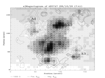
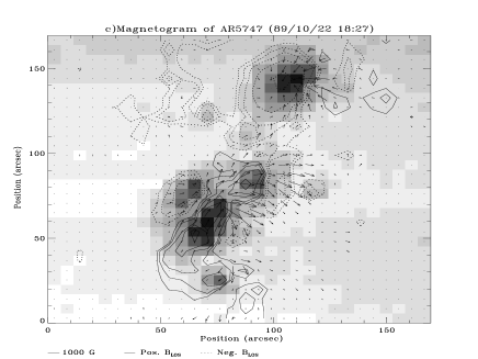
Figure 1: Three MSO vector magnetograms of AR 5747 superposed on white light images taken on Oct. 20–22, 1991. In all the figures, the solid lines stand for positive polarities and the dotted lines for negative polarities. The contour levels correspond to 100, 200, 400, 800 and 1600 G, respectively. The length of arrows represents the magnitude of the transverse field components.

Figure 1 shows the ambiguity resolved vector magnetograms obtained on Oct. 20 to Oct. 22, 1989. The three magnetograms have the same field of view. As seen in the figures, strong sheared transverse fields are concentrated near the neutral line and they form a global clockwise winding pattern. In Paper I, an account is given of the magnetic nonpotentiality parameters used in this study. The vertical current density is presented in Figure 2. The vertical current density kernels persisted, with little change of configuration, over the whole observing span. Wang, Xu, and Zhang (1994) and Leka et al. (1993) have discussed the important characteristics of these vector magnetic fields and vertical current densities. We tabulate the time variation of magnetic fluxes and total vertical currents of positive and negative signs in Table III. The differences between the absolute values of the positive and negative quantities are within a few percent. As seen in the table, the magnetic fluxes and total vertical currents of both signs decreased with time. It is observed that several small $\delta$ sunspots (A1, A2 and A3 in Fig. 1a) disappeared in Figure 1b, which suggests that flaring events between Oct. 20 and 21 should be associated with flux cancellation. It is to be noted that there were no remarkable flux emergence during the observing period.

Table III: Magnetic fluxes and total vertical currents in AR 5747 for three different times in the observing period. Here $\sigma_{J}$ denotes the standard deviation of the vertical current distribution.

Data	Flux(+) [Mx]	Flux(-) [Mx]	$\sum J_{z}^{+}[\rm A]$	$\sum J_{z}^{-}[\rm A]$	$\sigma_{J}[\rm mA/m^{2}]$
a)	1.56E22	1.51E22	6.7E4	6.6E4	1.4
b)	1.31E22	1.28E22	4.2E4	4.2E4	1.2
c)	0.92E22	0.89E22	3.9E4	4.0E4	1.2

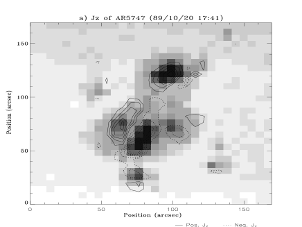
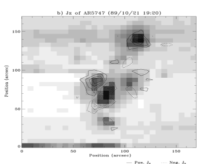
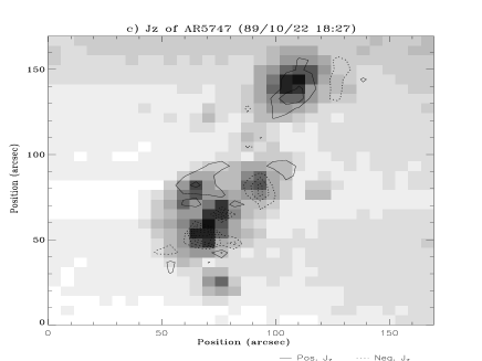
Figure 2: Contours of vertical current density in AR 5747. The contour levels correspond to 3, 6, 9, 12 and 15 $\rm mA/m^{2}$, respectively. In all the panels, the solid lines stand for positive vertical current density and the dotted lines for negative current density.

Table IV: Field strength weighted mean magnetic shear angle $\overline{\theta}_{s}$, transverse field weighted angular shear $\overline{\theta}_{a}$, mean free energy density $\overline{\rho}_{f}$, planar sum of magnetic free energy density $\sum\rho_{f}$, and $\sum({\rm MAD}\times|{\bf B}|)$ for AR 5747 for three different times. The values in parentheses are obtained employing the potential field method.

Data	$\overline{\theta}_{s}$	$\overline{\theta}_{a}$	$\overline{\rho}_{f}$	$\sum\rho_{f}$	$\sum({\rm MAD}\times|{\bf B}|)$
a)	46.8(38.4)	71.8(56.1)	2.7(2.0)E4	1.4(1.0)E24	4.7E6
b)	41.3(36.3)	63.0(53.4)	2.1(1.6)E4	9.3(6.9)E23	3.5E6
c)	36.1(32.6)	55.7(48.3)	1.7(1.4)E4	5.1(4.3)E23	2.3E6

Figure 3: Contours of angular shear multiplied by transverse field strength drawn in thick solid lines are superposed on longitudinal magnetograms. The contour levels are $4.0\times 10^{4}$, $7.0\times 10^{4}$, $1.0\times 10^{5}$ and $1.3\times 10^{5}\,\rm G\,deg$, respectively. In all the panels, the solid lines stand for positive longitudinal polarities and the dotted lines for negative ones. The contour levels in the magnetograms correspond to 100, 200, 400, 800 and 1600 G, respectively.

Figure 4: Contours of shear angle multiplied by field strength drawn in thick solid lines are superposed on longitudinal magnetograms. The contour levels are $4.0\times 10^{4}$, $7.0\times 10^{4}$, $1.0\times 10^{5}$ and $1.3\times 10^{5}\,\rm G\,deg$, respectively. The magnetograms are the same as in Figure 3.

Figure 5: Contours of free energy density drawn in thick solid lines are superposed on magnetograms. The contour levels are $5.0\times 10^{4}$, $1.0\times 10^{5}$, $1.5\times 10^{5}$, $2.0\times 10^{5}$ and $2.5\times 10^{5}\,\rm erg/cm^{3}$, respectively. The magnetograms are the same as in Figure 3.

Figure 6: Contours of MAD multiplied by field strength drawn in thick solid lines are superposed on longitudinal magnetograms. The contour levels are $3.0\times 10^{4}$, $5.0\times 10^{4}$, $7.0\times 10^{4}$, $9.0\times 10^{4}$ and $1.1\times 10^{5}\,\rm G\,deg$, respectively. The magnetograms are the same as in Figure 3.

Figure 3 shows the angular shear multiplied by transverse field strength and Figure 4 shows the shear angle multiplied by total field strength. As seen in the figures, strong magnetic shear is concentrated near the inversion line, where ${\rm H}_{\beta}$ emission patches were observed (see Fig. 2 of Wang, Xu, and Zhang 1994). The time variation of two weighted mean shear angles is given in Table IV. The values of two shear angles monotonically decreased with time. The magnetic free energy density is shown in Figure 5. Its evolutionary trend is quite similar to that of shear angles. The 2-D MAD multiplied by total field strength (Figure 6) also has a similar evolutionary pattern to that of the other nonpotentiality parameters above. We summarize the variations of mean free energy density, planar sum of free energy density, and sum of MAD multiplied by field strength in Table IV, in which the values obtained with the potential field method for the $180^{\circ}$ ambiguity resolution are also given in parentheses for comparison. As seen in the table, all the nonpotentiality parameters under consideration decreased with time, which suggests that the active region was in a relaxation stage during the observing period.

From the above results, we may infer that the flares that occurred in our observation are just bursty parts of energy release in a long term relaxation of the stressed magnetic field. In a self-organizing system, a transition toward a lower energy state proceeds very mildly in the beginning and for most of time until a sudden bursty event develops as in an avalanche. Why, then, did a series of flares occur, rather than one? Flares can surely take place in repetition if enough energy is supplied into the system between the flaring events to recover the free energy released by the preceding flaring event. However, this is not the case as far as the flares in our observation are concerned. No indication of energy input, whether flux emergence or increase of magnetic shear, was detected throughout our observing span. We thus speculate that the occurrence of a series of flares was possible due to the complex geometry of our active region magnetic field. A simple bipolar magnetic field would proceed to a lower energy state by one bursty event of reconnection. However, in a complex active region containing more than a pair of magnetic poles, the transition to the lowest energy state may possibly comprise several steps of macroscopic change in field topology. This speculation, of course, has to be examined by further studies involving many other observations and numerical experiments as well.

Section 4 Magnetic Forces and Linear Force-Free Field Approximation

It is generally believed that solar magnetic fields are force-free in the corona, but far from it in the photosphere. However, to construct a force-free model of the coronal magnetic field, the field data observed at the photospheric level are employed as boundary conditions. Not only because a magnetohydrostatic equilibrium under gravity is more difficult to construct than a force-free solution, but also because no reliable information about plasma pressure is available in the photosphere, force-free field modeling with photospheric boundary conditions is being widely attempted (e.g., McClymont and Mikić, 1994 for AR 5747) despite the afore-mentioned inconsistency. The reliability of such models thus depends on how much the field behaves like a force-free field near the photosphere. In this section, we investigate the “force-freeness” of AR 5747.

A force-free field is a magnetic field satisfying the Lorentz force-free condition

$$(\nabla\times{\bf B})\times{\bf B}=0\,,$$ (1)

which can be rewritten as

$$\nabla\times{\bf B}=\alpha{\bf B}\,.$$ (2)

The so called force-free coefficient $\alpha$ is thus given by

$$\alpha={J_{x}\over B_{x}}={J_{y}\over B_{y}}={J_{z}\over B_{z}}\,,$$ (3)

in rationalized electromagnetic units. Taking divergence of Equation (2) and using $\nabla\cdot{\bf B}=0$, we have

$${\bf B}\cdot\nabla\alpha=0\,,$$ (4)

which means that $\alpha$ is a function of each field line. With the vector magnetogram of Oct. 20, 1989, Canfield et al. (1991) examined whether the ratio of current density to field strength ($J/B$) is conserved along each elementary flux tube. Although the force-free coefficient $\alpha=J_{i}/B_{i}$ is necessarily constant along each field line in a force-free field, the condition is in practice difficult to check due to the noises in current density in weak field regions (McClymont, Jiao, and Mikić, 1997). To examine the force-freeness of AR 5747, we have computed the integrated Lorentz force components scaled with the integrated magnetic pressure force, i.e., $F_{x}/F_{o}$, $F_{y}/F_{o}$ and $F_{z}/F_{o}$ (Metcalf et al. 1995), in which

$$F_{x}=-{1\over 4\pi}\int B_{x}B_{z}dxdy,$$ (5)

$$F_{y}=-{1\over 4\pi}\int B_{y}B_{z}dxdy,$$ (6)

$$F_{z}=-{1\over 8\pi}\int(B_{z}^{2}-B_{x}^{2}-B_{y}^{2})dxdy,$$ (7)

and

$$F_{o}={1\over 8\pi}\int(B_{z}^{2}+B_{x}^{2}+B_{y}^{2})dxdy,$$ (8)

where $F_{o}$ is the integrated magnetic pressure force. In this calculation, only pixels with field strength larger than 100 G for both longitudinal and transverse fields are considered to reduce the effect of noise. In Table V, we present the normalized integrated forces obtained from three vector magnetograms. The absolute values of these forces are much smaller than those at the photospheric level of Metcalf et al. (1995), which implies that our active region field is more or less force-free even near the solar surface. It is also noted that the magnetic fields of AR 5747 become less force-free in a relaxation stage as times go.

Table V: Normalized integrated forces and linear force free coefficients for AR 5747.

	Data	$F_{x}/F_{o}$	$F_{y}/F_{o}$	$F_{z}/F_{o}$	$\alpha\rm[m^{-1}]$	$\alpha^{*}$
	a)	0.008	0.005	-0.126	-1.1$\times 10^{-7}$	-6.8$\times 10^{-8}$
	b)	0.042	0.015	-0.148	-1.0$\times 10^{-7}$	-6.1$\times 10^{-8}$
	c)	0.097	0.085	-0.222	-7.2$\times 10^{-8}$	-4.5$\times 10^{-8}$

Asterisked (*) values are obtained by minimizing the difference between the horizontal components of the constant $\alpha$ force-free model and the observed horizontal magnetic fields, considering only pixels with $B_{t}>300\,\rm G$ (Pevtsov et al. 1996).

Figure 7: $J_{z}$ vs. $B_{z}$ from three vector magnetograms of AR 5747. Straight lines are the regression lines obtained from eye fitting.

Now we turn to the question whether our active region field is approximately linearly force-free. In Figure 1, the transverse field vectors show a common curling pattern for each magnetic polarity, which allows us to expect that values of the force-free coefficient do not diverge much. To investigate the linearity, we have plotted for each data set $B_{z}$ vs. $J_{z}$ and a plausible regression line obtained by eye fitting in Figure 7. The figures show that there exist approximate linear relationships between $B_{z}$ and $J_{z}$ for three vector magnetograms. We have already observed in Figures 1 and 2 that the distribution of vertical electric current density well matches that of magnetic fluxes of opposite polarity. In Table V, we have tabulated linear force-free coefficients obtained by linear regression in Figure 7. We have also listed the coefficients obtained by minimizing the difference between the horizontal components in a constant $\alpha$ force-free field model and the horizontal field vectors in the vector magnetogram, considering only pixels with $B_{t}>300\,\rm G$ (Pevtsov et al., 1996). In both sets, the absolute value of force-free coefficients decreased with time, as other nonpotentiality parameters did. This suggests that the linear force-free coefficient could be as good a nonpotential evolutionary indicator as other nonpotentiality parameters as long as the linear force-free approximation is more or less valid. Furthermore, the linear force-free coefficient has a merit as a global parameter.

Section 5 Summary and Conclusion

In this study, we have analyzed the MSO vector magnetograms of AR 5747 taken on October 20 to 22, 1989. A nonlinear least square method was adopted to derive the magnetic field vectors from the observed Stokes profiles and a multi-step ambiguity solution method was used to resolve the $180^{\circ}$ ambiguity. From the ambiguity-resolved vector magnetograms, we have derived a set of physical quantities which are magnetic flux, vertical current density, magnetic shear angle, angular shear, magnetic free energy density and MAD, a measure of magnetic field discontinuity. In order to examine the force-free character of the active region field, we have calculated the normalized integrated Lorentz forces and compared the longitudinal field $B_{z}$ and the corresponding vertical current density $J_{z}$. Most important results from this work can be summarized as follows.

1) Magnetic nonpotentiality is concentrated near the inversion line, where flare brightenings are observed.

2) All the physical parameters that we have considered (vertical current density, mean shear angle, mean angular shear, sum of free energy density and sum of MAD) decreased with time, which indicates that the active region was in a relaxation period.

3) The X-ray flares that occurred during the observing period could be related with flux cancellation. Flaring events might be considered as bursty parts in the long term relaxation process.

4) It is found that the active region was approximately linearly force-free throughout the observing span and the absolute value of the derived linear force-free coefficient decreased with time. Our result suggests that the linear force-free coefficient could be a good global parameter indicating the evolutionary status of an active region as long as the field is approximately force-free.

References

- Canfield et al. 1991 Canfield, R. C., Fan, Y. , Leka, K. D., Lites, B. W., and Zirin, H.: 1991, in Solar Polarimetry, Proceeding of the Workshop of Solar Polarimetry, ed. L. November , p. 296.
- Canfield et al. 1993 Canfield, R. C., La Beaujardiere, J.-F., Han, Y., Leka, K. D., McClymont, A. N., Metcalf, T. R., Mickey, D. L., Wulser, J.-P., and Lites, B. W.: 1993, Astrophys. J. 411, 362.
- Hagyard et al. 1984 Hagyard, M. J., Smith, Jr., J. B., Teuber, D., and West, E. A.: 1984, Solar Phys. 91, 115.
- Hagyard et al. 1990 Hagyard, M. J., Ventkatarishnan, P., and Smith, Jr., J. B.: 1990, Astrophys. J. Suppl. 73, 159.
- Leka et al. 1993 Leka, K. D., Canfield, R. C., McClymont, A. N., de la Beaujardiere, J. F., and Fan, Y.: 1993, Astrophys. J. 411, 370.
- McClymont and Mikić 1994 McClymont, A. N. and Mikić, Z.: 1994, Astrophys. J. 422, 899.
- McClymont, Jiao, and Mikić 1997 McClymont, A. N., Jiao, L., and Mikić, Z.: 1997, Solar Phys. 174, 191.
- Metcalf et al. 1991 Metcalf, T. R., Canfield, R. C., Mickey, D. L., and Lites, B. W.: 1991, in Solar Polarimetry, Proceeding of the Workshop of Solar Polarimetry, ed. L. November , p. 376 .
- Metcalf et al. 1995 Metcalf, T. R., Jiao, L., McClymont, A. N., Canfield, R. C., and Uitenbroek, H.: 1995, Astrophys. J. 439, 474.
- Mickey 1985 Mickey, D. L.: 1985, Solar Phys. 97, 223.
- Moon et al. 1999a Moon, Y.-J., Yun, H. S., Lee, S. W., Kim, J.-H. Choe, G. S., Park, Y. D., Ai, G., Zhang, H., and Fang, C.: 1999a, Solar Phys. 184, 323.
- Moon, Park, and Yun 1999b Moon, Y.-J., Park, Y. D., and Yun, H. S.: 1999b, J. Korean Astron. Soc. 32, 63.
- Moon et al. 1999c Moon, Y.-J., Yun, H. S., Choe, G. S., Park, Y. D., and Mickey, D. L.: 1999c, submitted to Solar Physics. (Paper I)
- Pevtsov et al. 1996 Pevtsov, A. A., Canfield, R. C., and Zirin, H.: 1996, Astrophys. J. 473, 533.
- Pevtsov et al. 1997 Pevtsov, A. A., Canfield, R. C., and McClymont, A. N.: 1997, Astrophys. J. 481, 973.
- Ronan et al. 1987 Ronan, R. S., Mickey, D. L., and Orral, F. Q.: 1987, Solar Phys. 113, 353.
- Skumanich and Lites 1987 Skumanich, A and Lites, B. W.: 1987, Astrophys. J. 322, 473.
- Wang 1997 Wang, H.: 1997, Solar Phys. 174, 163.
- Wang et al. 1996 Wang, J., Shi, Z., Wang, H., and Lue, Y.: 1996, Astrophys. J. 456, 861.
- Wang et al. 1994 Wang, T., Xu, A., and Zhang, H.: 1994, Solar Phys. 155. 99.