STUDY OF SOLAR ACTIVE REGIONS BASED ON BOAO VECTOR MAGNETOGRAMS
Abstract
In this study we present the study of solar active regions based on BOAO vector magnetograms and filtergrams. With the new calibration method we analyzed BOAO vector magnetograms taken from the SOFT observational system to compare with those of other observing systems. In this study it has been demonstrated that (1) our longitudinal magnetogram matches very well the corresponding Mitaka’s magnetogram to the extent that the maximum correlation yields r=0.962 between our re-scaled longitudinal magnetogram and the Mitaka’s magnetogram; (2) according to a comparison of our magnetograms of AR 8422 with those taken at Mitaka solar observatory their longitudinal fields are very similar to each other while transverse fields are a little different possibly due to large noise level; (3) main features seen by our longitudinal magnetograms of AR 8422 and AR 8419 and the corresponding Kitt Peak magnetograms are very similar to each other; (4) time series of our vector magnetograms and H-alpha observations of AR 8419 during its flaring (M3.1/1B) activity show that the filament eruption followed the sheared inversion line of the quadrupolar configuration of sunspots, indicating that the flare should be associated with the quadrupolar field configuration and its interaction with new filament eruption. Finally, it may be concluded that the Solar Flare Telescope at BOAO works normally and it is ready to do numerous observational and theoretical works associated with solar activities such as flares.
I INTRODUCTION
It is well known that magnetic fields play an important role in solar active phenomena such as solar flares and prominences. However, measurements of magnetic fields are only available at the photosphere and very limitedly at the chromosphere. Thus the evolution of magnetic fields at the photosphere has widely used for studies of relationships between active phenomena and magnetic fields. In this sense, reasonable measurements of solar magnetic fields at the photospheric level are of key importance in understanding solar activities (e.g. Hagyard et al. 1984).
Solar Flare Telescope (SOFT) has been set up at the peak of Mt. Bohyun in 1995. A filter-based magnetograph (Vector Magnetograph, VMG) is attached to the SOFT (Moon 1999c, Park et al. 1997) of Bohyunsan Optical Astronomy Observatory (BOAO), which uses a very narrow band Lyot (birefringent) filter which measures magnetic fields at the solar photosphere with Fe I 6302.5 line. The Stokes parameters are measured by collecting spectrally integrated data over the filter passband. It has very high time resolution which is less than 1 minute, with relatively large field of view (). For the efficient use of the SOFT, we have developed the data acquisition system (Moon et al. 1996), the telescope control software (Moon et al. 1997), the KD*P control system (Nam et al. 1997), and the four channel filter control system (Jang et al. 1998).
The calibration problem of filter-based magnetographs with Fe I 6302.5 spectral line has been discussed by several authors (Ichimoto 1993, Sakurai et al. 1995, Kim 1997, Moon et al. 199b). Recently, Moon et al. (1999b) have developed an improved calibration method by using theoretical Stokes polarization signals calculated with various inclination angles of magnetic fields (Hagyard and Kineke 1995).
In this paper we study solar active regions using BOAO vector magnetograms with the new calibration method. For this we describe how to analyze BOAO vector magnetograms in Section II and compare observed magnetograms with corresponding magnetograms from other solar observatories in Section III. In Section IV we present some observational results of AR 8419 by the SOFT. A brief summary and conclusion will be given in Section V.
II ANALYSIS OF VECTOR MAGNETOGRAMS
(a) Dark Frame and Flat Field Correction
For detecting observed images through VMG we use a SONY-XC 77 video CCD, whose signal is digitized by the image processor (Moon et al. 1996). Dark frame observations are made by closing the cover of the telescope. Flat field observations were made by calibration optics to produce defocused lights. However, the observed flat images had relatively large intensity gradients so that we now use a defocused intensity image of the solar disk center as a flat image by adjusting a focusing motor.
The dark frame (D) and flat field (F) corrections are made by
| (1) |
| (2) |
where represents an observed image and , the image corrected for dark frame and flat field. We found that there are little systematic difference between and . In Stokes V/I observation, a final image corrected for dark frame and flat field can be expressed as
| (3) |
where we assume that . This argument can be also applied to Stokes Q/I and U/I observations. These facts imply that flat field correction can be neglected in magnetic field observations.
(b) Alignment of Q, U, V Images
Due to atmospheric seeing and tracking instability, observed images could be shifted during filter turret transition for Q, U, and V observations. When we make an observation of a set of Stokes data, three FITS files for Q, U and V are obtained, in which and are separately saved. Here and correspond to a filter convolved monochromatic intensity of right and left hand polarization, respectively. For convenience we define three intensity images as follows : in Q data, in U data, and in V data. We usually make alignments of theses intensity images by shifting and images to match an image as follows. (1) Two set of coordinates for the same largest sunspots in both a target image ( or ) and a reference image () are searched by the center of gravity method (Ichimoto 1993). (2) An appropriate size of window around the coordinates are determined. (3) The target image is shifted to have a maximum correlation with the reference image for the selected window.
(c) Calibration
Moon et al. (1999b) have already discussed the calibration problems of filter-based magnetograms, especially focusing on the Fe I 6302.5 spectral line for the SOFT. In applying our developed method to the actual analysis the following facts should be kept in mind. In many cases, magnetic field strengths derived from filter-based magnetographs have been underestimated relative to theoretically predicted or spectrally determined ones. To compensate this problem, an arbitrary factor, so called k-factor, has been introduced to raise the observed polarization signals so that it matches the field strength estimated from nonfilter-based magnetic observations (Gary et al. 1987, Chae 1996). According to Chae (1996), stray light corrected fields still require a k-factor to match empirically determined ones. The underestimation of magnetic fields might be due to stray light effect (Chae et al. 1998a, 1998b), instrumental depolarization (Gary 1991), the fragmental distribution of the magnetic field on the solar surface (Ichimoto 1993), and transmission wavelength error etc. To properly correct all the problems related to this matter seems to be too challenging.
For the calibration of BOAO magnetograms, we suggest to select one of two methods. The first method is a calibration method for Mitaka Solar Observatory (Ichimoto 1993, 1997, Sakurai et al. 1995), which is applicable to BOAO vector magnetograms since two observational systems are very similar to each other. Here we summarize Mitaka’s method as follows. (1) Observed polarization signals are converted to magnetic field strengths by the method described in Ichimoto (1993). (2) A k-factor is multiplied to longitudinal fields to balance between observed transverse fields and corresponding potential fields derived from the observed longitudinal fields (Sakurai et al. 1995). First, potential magnetic fields are derived by using a Fourier expansion method (Sakurai 1992) in which observed longitudinal fields are used as a boundary condition. Then they select data points on which the observed and the computed transverse fields have the nearly same directions, and compute the average ratio of the observed and computed transverse field strengths. Finally, this ratio (k-factor) is multiplied to the observed longitudinal fields to produce re-scaled longitudinal ones. In addition, we re-scale the calibrated vector fields to balance between the maximum of longitudinal fields and that of corresponding fields from a full disk longitudinal magnetogram of Kitt Peak Solar Observatory, which have provided us with unique daily full disk longitudinal magnetograms by the NSO/KP Vacuum Telescope together with a 10.7m vertical Littrow spectrograph (Jones et al. 1992).
In terms of sunspot models as well as observational data of active regions, we have tested the validity of the second process that transverse fields balance with corresponding potential fields derived from longitudinal fields. First, we computed k-factors for three sunspot models which well describe observed field configuration at the photosphere and computed values are found to be 1.12 for Skumanich (1992)’s dipole model, 1.09 for Yun(1970)’s sunspot model, and 1.05 for Moon et al. (1998)’s sunspot model. We have also computed k-factors for 37 vector magnetograms of four flare-productive active regions (AR 5747, AR 6233, AR 6659, and AR 6982) observed at Mees Solar Observatory whose Stokes polarimeter is one of qualified spectrometer-based magnetographs. It is found that computed values for 28 magnetograms (about 76%) out of 37 are approximately unity within 10% accuracy. These results imply that the second process could be applied to representative active regions.
The second calibration method is to employ the iterative calibration method (Moon et al. 1999b), which only works as long as both circular and linear polarization signals are reasonably estimated. Unfortunately, underestimation of circular polarization signals are larger than that of linear polarization ones. Thus we have devised an iterative method for calibration as follows. (1) We follow two-steps (1) and (2) of the first calibration method and multiply a derived k-factor to circular polarization signals. (2) We convert both re-scaled circular and original linear polarization signals to vector fields by our developed calibration method described in Moon et al. (1999b). (3) We re-scale longitudinal fields by the step (2) of the first method. (4) We iterate steps (2) and (3) until a k-factor (re-scaling factor) converges unity within 5 % accuracy. (5) If necessary, we re-scale again the calibrated vector fields to balance between the maximum of longitudinal fields and that of corresponding fields from a full disk longitudinal magnetogram of Kitt Peak Solar Observatory.
(d) Solutions for ambiguity
When one analyzes vector magnetograms from solar magnetograph measurements, one of challenging problems is to solve the ambiguity in the azimuth of observed transverse fields. This ambiguity is attributed to the fact that two anti-parallel polarization signals of transverse fields are indistinguishable each other since the transverse measurements of the magnetograph provides only the plane of linear polarization. For all vector magnetograms the ambiguity should be resolved to obtain the correct transverse field components. The great importance of the problem is attributed to the fact that the reasonable resolution of the problem can give us a meaningful understanding on physical quantities such as vertical current density, shear angle, magnetic free energy.
To resolve the ambiguity, an additional constraint on the field azimuth should be introduced in terms of theoretical or observational aspects. One of commonly used ways is the potential field method based on the fact that an observed transverse magnetic field is not far away from a corresponding potential component. That is, the direction of the transverse field is chosen such that the two transverse components make an acute angle. This method holds for for nearly potential regions but not for highly non-potential regions.
For our study we adopt two ambiguity methods : a potential field method (Sakurai 1992) and a multi-step method (Canfield et al. 1993). Comprehensive reviews for resolving the problem are found in several literatures (e.g., Sakurai 1989, Wang 1993, Gary and Demoulin 1995).
i) Potential Field Method
For the case of a potential field, the magnetic field can be derived from a scalar potential ,
| (4) |
Using , the potential should satisfy the Laplace’s equation:
| (5) |
where an observable quantity is used as the boundary condition, .
The potential field solution was initially suggested by Schmidt (1964) with the use of the Green function method. Later, the Fourier expansion method has been employed by Teuber et al.(1977) and Sakurai(1989). For our study, we have used a Fourier expansion method developed by Sakurai (1992). The criterion of the method is given by
| (6) |
where is an observed transverse field and is a tangential component of the potential field solution derived from Equation (5).
ii) Multi-step Method
Canfield et al. (1993) employed a multi-step for ambiguity solution, which was well described in the Appendix of their paper. Here we summarize their method as follows. Step 1 : They first choose the orientation of each transverse field vector which is closest to the potential field computed using longitudinal fields as a boundary condition. Then they rotate the data to the heliographic coordinate system. Step 2 : For current-carrying active regions, after resolving with the potential field, they compute the linear force-free field with a linear force-free coefficient selected to match nonpotentialities discovered in Step 1. Step 3 : They next choose the orientation of the transverse field which minimizes the angle between neighboring field vectors by maximizing the sum of the vector dot product of the field vector with each of its eight neighbors. Step 4 : In regions with strong total magnetic field strength () and a high degree of shear (transverse field azimuth differing from the potential azimuth by more than ), they iteratively select the orientation of the field which minimizes the field divergence . Step 5 : Finally, in regions where the total field strength is below the noise level in the magnetograms, they iteratively choose the orientation of the field which minimizes the electric current.
III COMPARISON WITH OTHER MAGNETOGRAMS
We have compared vector fields of AR 8422 with corresponding magnetogram of Mitaka Solar Telescope (Sakurai et al. 1995) which have produced qualified vector magnetograms since 1992. The comparison seems to be more meaningful in that instruments and detecting system of the Mitaka Solar Observatory are very similar to those of the SOFT in BOAO.
For comparison we adopted the first calibration method, i.e., the standard reduction procedure of Mitaka Observatory (Ichimoto 1993, 1997), and the multi-step method (Canfield et al. 1993) for the ambiguity resolution.
A field of view ( ) of VMG in the SOFT was originally determined from its optical layout. Since the optical layout have been a little changed so that its field of view needs to be redetermined. In the case of Mitaka’s magnetograms, its field of view was determined by using a stop tracker (Ichimoto 1993). We have determined a field of view of vector magnetogram made with VMG by comparing with Mitaka’s corresponding magnetograms as follows. First of all, we have made a linear matching of SOFT’s magnetogram with Mitaka’s corresponding magnetogram for AR 8422 (S23W38) on Dec. 28, 1998. For this we make a linear mapping of reference magnetogram over the image coordinate system of corresponding magnetogram under consideration (Chae 1999):
| (7) |
| (8) |
where and are coordinates of data points in a considered magnetogram in unit of pixel, and and are coordinates of the corresponding points in a reference magnetogram. Chae (1999) determined four parameters by minimizing
| (9) |
over , , , and , where is a target magnetogram and is a re-mapped reference magnetogram.
We applied Chae’s method to a longitudinal magnetogram of AR 8422 observed on Dec. 28, 1998 and corresponding Mitaka’s magnetogram. We have also developed another method which derive i, j, l, and m to have a maximum correlation between and . Two methods are in good agreements with each other, as expected. The field of view () of our observed vector magnetogram has been confirmed by finding the maximum correlation between our remapped longitudinal magnetogram and corresponding Mitaka’s magnetogram within about 1%. Figure 1 shows the comparison of BOAO’s longitudinal magnetic fields of AR 8422 and corresponding magnetic fields made with a similar magnetograph at Mitaka Solar Observatory. As seen in the figure, they are well correlated with each other (r=0.962). Some differences in negative strong field regions may be due to seeing condition, tracking instability, filter transmission wavelength, and observational time difference etc.
Figure 2 shows BOAO(upper) and Mitaka(lower) vector magnetic fields of AR 8422 observed on Dec. 28, 1998. Its main features of longitudinal fields are very similar to each other, while those of transverse fields are a little different, which might be due to large noise levels ( G) of transverse fields.


In Figure 3 we present a longitudinal magnetogram observed on Dec. 27, 1998 at Kitt Peak Solar Observatory. Even though it was obtained about eight hours before than the corresponding SOFT’s one (Figure 2-a)), its main features are very similar to those of SOFT’s one. Our study shows that our vector magnetograph should normally work.


IV STUDY OF ACTIVE REGION AR 8419
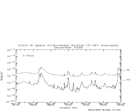
We have observed vector fields together with and white light of flare producing active region AR 8419 (N27W27) in which a M-class flare (M3.1/1B) occurred on Dec. 28, 1998. According to Solar Geophysical Data, GOES X-ray flux started to increase at UT 05:45, peaked at UT 05:48, and then ended at UT 05:59 (See Figure 4).
At that time, the active region was of very complex magnetic polarities ( type). Figure 5 shows two vector magnetograms observed before and after the flare. The magnetograms were calibrated by the second calibration method in Section II. According to NOAA reports, this region has grown in complexity as well as in sunspot area for three days with sizable proceeding (P1 in Figure 5) and following sunspot (N1). The following sunspot has a series of umbra forming a NE-SW line with surrounding penumbra with a configuration (N1 and P2).
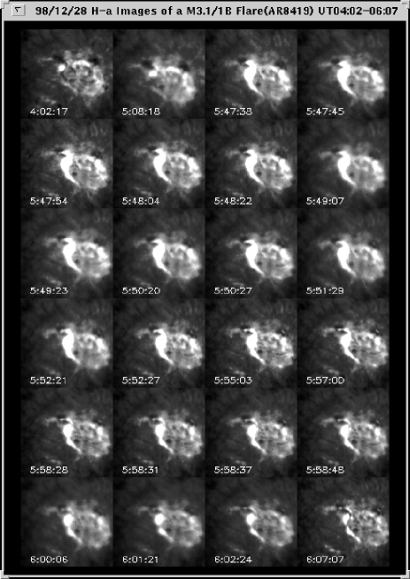
Figure 6 shows a time series of filtergrams of the SOFT for about two hours including the peak time of X-ray fluxes. In the figures two dark areas correspond to the proceeding (P1) and following (N1) sunspots. At UT 4:02, two small brightening patches were found near the sunspot region. At UT 05:47, strong inverse -shape (Pevtsov et al. 1997) H patches were notified and last for about ten minutes, and then remained several flare ribbons.
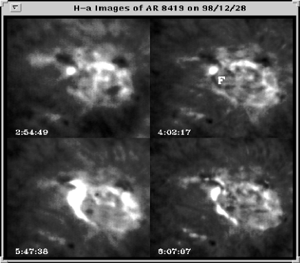
In order to examine in detail the change of H phenomena, we present four filtergrams observed before and after the flare in Figure 7. It is interesting to note that there was a filament eruption with inverse -shape (denoted by F on the 4:02 image), which exactly match the inversion line of a quadrupolar configuration (P2, P3, N1, N2 in Figure 5). As seen on 06:07 image, several flare ribbons are made after an eruptive phase of the flare. It is well accepted that two flare ribbons in emission are a result of filament eruption along the inversion line of configuration region (Priest 1982, Zirin 1988, Filippov 1997). We suggest that the M-class flare in AR 8419 should be associated with the quadrupolar configuration and its interaction with the new erupting filament.
It is also found that sunspots in the quadrupolar configuration were nearly in a straight line with the largely sheared inversion line (Figure 5), which was often observed in flare producing active regions (Demoulin, Hénoux, and Mandrini 1994). Moon et al. (1999a) showed that a large magnetic field discontinuity exist at the separator of such a quadrupolar configuration that directions of two bipoles are antiparallel each other ( in Table 1 of their paper).
Figure 8 shows two longitudinal magnetograms of AR 8419 observed on Dec. 27 and 28, 1998 at Kitt Peak Solar Observatory. Its main features are very similar to those of SOFT’s corresponding ones in Figure 5. The comparison of Figure 5 and 8-a) shows that a positive polarity sunspot (P2) moved westward, collide with the following sunspot (N1) to form a configuration and to compress longitudinal fields near the configuration. In Figure 5, steep longitudinal field gradients over horizontal direction are notified and estimated to be about 0.2 G/km near the sunspot, which was often reported in flare-producing active regions (e.g., Patty and Hagyard 1986, Zhang et al. 1994 ). It is also found that the inversion line with inverse -shape become more twisted after the flare.
V SUMMARY AND CONCLUSION
We have compared our vector fields of AR 8422 with those made with a similar vector magnetograph at Mitaka solar observatory. The comparison shows that longitudinal fields are very similar to each other but transverse fields are a little different. We have also compared longitudinal magnetograms of AR 8422 and AR 8419 with Kitt Peak longitudinal magnetograms and confirmed that its main features are very similar to those of the SOFT.
We have also presented our vector magnetograms and H observations of AR 8419 during its flaring(M3.1/1B) activity. Time series H-alpha observations show a filament eruption following the sheared inversion line of the quadrupolar configuration of sunspots and an inverse -shape brightening patch near the filament. This fact imply that this flare could be associated with the quadrupolar configuration and its interaction with the filament eruption.
ACKNOWLEDGEMENTS We wish to thank Dr. Ichimoto and Dr. Sakurai for allowing us to use some of their numerical routines for data analysis. This work has been supported in part by the Basic Research Fund (99-1-500-00 and 99-1-500-21) of Korea Astronomy Observatory and in part by the Korea-US Cooperative Science Program under KOSEF(995-0200-004-2).
REFERENCES
Canfield, R. C., La Beaujardiere, J.-F., Han, Y., Leka, K. D., McClymont, A.N., Metcalf, T. R., Mickey, D.L., Wuelser, J-P., & Lites, B.W. 1993, ApJ, 411, 362
Chae, J. 1996, Ph.D. dissertation, Seoul National University
Chae, J., Yun, H. S., Sakurai, T., & Ichimoto, K. 1998a, Sol. Phys.183, 229
Chae, J., Yun, H. S., Sakurai, T., & Ichimoto, K. 1998b, Sol. Phys.183, 245
Chae, J. 1999, private communication
Demoulin, P., Hénoux, J. C. and Mandrini, C. H. 1994, A&A, 285, 1023
Filippov, B. P. 1997, A&A, 324, 324
Gary, G. A., Moore, R. L., & Hagyard, M. J. 1987, ApJ, 314, 782
Gary, G. A., Hagyard, M. J., & West, E. A. 1991, in Solar Polarimetry, Proceeding of the Workshop of Solar Polarimetry, ed. L. November, p65
Gary, G. A. & Demoulin, P. 1995, ApJ, 445, 982
Hagyard, M.J., Smith, Jr, J.B., Teuber, D., & West, E. A. 1984, Sol. Phys., 91, 115
Hagyard, M.J. & Kineke, 1995, Sol. Phys., 158, 11
Ichimoto, K. 1993, in his solar magnetic field computation package
Ichimoto, K. 1997, private communication
Jang, B.-H., Nam, O.W. Park, Y.D., Han, I. W., Moon, Y.-J. 1998, KAO technical Report, Development of four channel filter controlling system
Jones, H. P., Duvall, Jr. T. R., Harvey, J. W., Mahaffey, C. T., Schwitters, J. D., & Simmons, J. E. 1992, Sol. Phys.139, 211
Kim, K. S. 1997, Pub. Kor. Astron. Soc. 12, 1
Moon, Y.-J., Park, Y.D., Jang, B.H., Sim, K. J., Yun, H. S., & Kim, J. H. 1996, Pub. Kor. Astron. Soc, 11, 243
Moon, Y.-J., Yoon, S.-Y., Park, Y.D.,& Jang, B.H. 1997, Pub. Kor. Astron. Soc, 12, 47
Moon, Y.-J., Yun, H. S., & Park, J.-S. 1998, ApJ, 494, 851
Moon, Y.-J., Yun, H.S., Lee, S.W., Kim, J.H., Choe, G., Park, Y.D., Ai, G. Zhang, H., & Fang, C. 1999a, Sol. Phys.184,
Moon, Y.-J., Park, Y. D., & Yun, H. S. 1999b, JKAS, 32, 63
Moon, Y.-J. 1999c, Ph. D. thesis, Seoul National University
Nam, O.W., Park, Y.D., Moon, Y.-J., and Kim, H.Y. 1997, KAO Technical Report, Development of a new KD*P control system
Park, Y.D., Moon, Y.-J., Jang, B-H., & Sim, K. J. 1997, Pub. Kor. Astron. Soc, 12, 35
Patty, S. R. & Hagyard, M. J. 1986, Sol. Phys.103, 111
Pevtsov, A.A., Richard, C.C., & McClymont, A. N. 1997, ApJ, 481, 973
Priest, E. R. 1982, in Solar Magnetohyrodynamics, (Dordrecht : Reidel )
Sakurai, T. 1989, Space Science Review, 51, 1
Sakurai, T. 1992, in his numerical routines
Sakurai, T., Ichimoto, K,. Nishino, Y., Shinoda, K., Noguchi, M., Hiei, E., Li, T., He, F., Mao, W., Lu, H., Ai, G., Zhao, Z., Kawakami, S., & Chae, J. 1995, PASJ, 47, 81
Schmidt, H. U. 1964, in Phys. of Solar Flares, ed. W.N. Hess, NASA SP-50, p107
Teuber, D. Tandberg-Hanssen, E., & Hagyard, M. J. 1977, Sol. Phys.53, 97
Wang, H. 1993, in Magnetic Field and Velocity Fields of Solar Active Regions, eds. H. Zirin, G. Ai, and H. Wang, ASP conference Series, 46, 323
Skumanich, A. 1992, in Sunspots : Theory and Observations, eds. J. H. Thomas and N. O. Weiss (Dordrecht: Kluwer Academic Publishers), 121
Yun, H. S. 1970, ApJ, 162, 975
Zhang, H., Ai, G., Yan, X., Li, W., & Liu, Y. 1994, ApJ, 423, 828
Zirin, H. 1988, in The Astrophysics of the Sun, Cambridge Univ. Press