The stellar populations of spiral galaxies

Abstract

We have used a large sample of low-inclination spiral galaxies with radially-resolved optical and near-infrared photometry to investigate trends in star formation history with radius as a function of galaxy structural parameters. A maximum likelihood method was used to match all the available photometry of our sample to the colours predicted by stellar population synthesis models. The use of simplistic star formation histories, uncertainties in the stellar population models and regarding the importance of dust all compromise the absolute ages and metallicities derived in this work, however our conclusions are robust in a relative sense. We find that most spiral galaxies have stellar population gradients, in the sense that their inner regions are older and more metal rich than their outer regions. Our main conclusion is that the surface density of a galaxy drives its star formation history, perhaps through a local density dependence in the star formation law. The mass of a galaxy is a less important parameter; the age of a galaxy is relatively unaffected by its mass, however the metallicity of galaxies depends on both surface density and mass. This suggests that galaxy mass-dependent feedback is an important process in the chemical evolution of galaxies. In addition, there is significant cosmic scatter suggesting that mass and density may not be the only parameters affecting the star formation history of a galaxy.

1 Introduction

It has long been known that there are systematic trends in the star formation histories (SFHs) of spiral galaxies; however, it has been notoriously difficult to quantify these trends and directly relate them to observable physical parameters. This difficulty stems from the age-metallicity degeneracy: the spectra of composite stellar populations are virtually identical if the percentage change in age or metallicity (Z) follows $\Delta{\rm age}/\Delta{\rm Z}\sim 3/2$ [Worthey 1994]. This age-metallicity degeneracy is split only for certain special combinations of spectral line indices or for limited combinations of broad band colours (Worthey 1994; de Jong 1996c; hereafter dJiv). In this paper, we use a combination of optical and near-infrared (near-IR) broad band colours to partially break the age-metallicity degeneracy and relate these changes in SFH with a galaxy’s observable physical parameters.

The use of broad band colours is now a well established technique for probing the SFH of galaxy populations. In elliptical and S0 galaxies there is a strong relationship between galaxy colour and absolute magnitude [Sandage & Visvanathan 1978, Larson, Tinsley & Caldwell 1980, Bower, Lucey & Ellis 1992, Terlevich et al. 1999]: this is the so-called colour-magnitude relation (CMR). This correlation, which is also present at high redshift in both the cluster and the field [Ellis et al. 1997, Stanford, Eisenhardt & Dickinson 1998, Kodama, Bower & Bell 1999], seems to be driven by a metallicity-mass relationship in a predominantly old stellar population [Bower, Lucey & Ellis 1992, Kodama et al. 1998, Bower, Kodama & Terlevich 1998]. The same relationship can be explored for spiral galaxies: Peletier and de Grijs [Peletier & de Grijs 1998] determine a dust-free CMR for edge-on spirals. They find a tight CMR, with a steeper slope than for elliptical and S0 galaxies. Using stellar population synthesis models, they conclude that this is most naturally interpreted as indicating trends in both age and metallicity with magnitude, with faint spiral galaxies having both a younger age and a lower metallicity than brighter spirals.

In the same vein, radially-resolved colour information can be used to investigate radial trends in SFH. In dJiv, radial colour gradients in spiral galaxies were found to be common and were found to be consistent predominantly with the effects of a stellar age gradient. This conclusion is supported by Abraham et al. [Abraham et al. 1998], who find that dust and metallicity gradients are ruled out as major contributors to the radial colour trends observed in high redshift spiral galaxies. Also in dJiv, late-type galaxies were found to be on average younger and more metal poor than early-type spirals. As late-type spirals are typically fainter than early-type galaxies (in terms of total luminosity and surface brightness; de Jong 1996b), these results are qualitatively consistent with those of Peletier & de Grijs [Peletier & de Grijs 1998]. However, due to the lack of suitable stellar population synthesis models at that time, the trends in global age and metallicity in the sample were difficult to meaningfully quantify and investigate.

In this paper, we extend the analysis presented in dJiv by using the new stellar population synthesis models of Bruzual & Charlot (in preparation) and Kodama & Arimoto (1997), and by augmenting the sample with low-inclination galaxies from the Ursa Major cluster from Tully et al. (1996; TVPHW hereafter) and low surface brightness galaxies from the sample of Bell et al. (1999; hereafter Paper i). A maximum likelihood method is used to match all the available photometry of the sample galaxies to the colours predicted by these stellar population synthesis models, allowing investigation of trends in galaxy age and metallicity as a function of local and global observables.

The plan of the paper is as follows. In section 2, we review the sample data and the stellar population synthesis and dust models used in this analysis. In section 3, we present the maximum-likelihood fitting method and review the construction of the error estimates. In section 4, we present the results and investigate correlations between our derived ages and metallicities and the galaxy observables. In section 5 we discuss some of the more important correlations and the limitations of the method, compare with literature data, and discuss plausible physical mechanisms for generating some of the correlations in section 4. Finally, we review our main conclusions in section 6. Note that we homogenise the distances of Paper i, dJiv and TVPHW to a value of $H_{0}=65$ kms^-1.

2 The data, stellar population and dust models

2.1 The data

In order to investigate SFH trends in spiral galaxies, it is important to explore as wide a range of galaxy types, magnitudes, sizes and surface brightnesses as possible. Furthermore, high-quality surface photometry in a number of optical and at least one near-IR passband is required. Accordingly, we include the samples of de Jong & van der Kruit (1994; dJi hereafter), TVPHW and Paper i in this study to cover a wide range of galaxy luminosities, surface brightnesses and sizes. The details of the observations and data reduction can be found in the above references; below, we briefly outline the sample properties and analysis techniques.

The sample of undisturbed spiral galaxies described in dJi was selected from the UGC [Nilson 1973] to have red diameters of at least 2 arcmin and axial ratios greater than 0.625. The sample presented in Paper i was taken from a number of sources [de Blok, van der Hulst & Bothun 1995, de Blok, McGaugh & van der Hulst 1996, O’Neil, Bothun & Cornell 1997a, O’Neil et al. 1997b, Sprayberry et al. 1995, Lauberts & Valentijn 1989, dJi] to have low estimated blue central surface brightnesses $\mu_{B,0}\ga$ 22.5 mag arcsec^-2 and diameters at the 25 B mag arcsec^-2 isophote larger than 16 arcsec. TVPHW selected their galaxies from the Ursa Major Cluster (with a velocity dispersion of only 148 km s^-1, it is the least massive and most spiral-rich nearby cluster): the sample is complete down to at least a $B$ band magnitude of $\sim$ 14.5 mag, although their sample includes many galaxies fainter than that cutoff. We take galaxies from the three samples with photometric observations (generously defined, with maximum allowed calibration errors of 0.15) in at least two optical and one near-IR passband, axial ratios greater than 0.4, and accurate colours (with errors in a single passband due to sky subtraction less than 0.3 mag) available out to at least 1.5 $K$-band disc scale lengths. For the Ursa Major sample, we applied an additional selection criterion that the $K^{\prime}$ band disc scale length must exceed 5 arcsec, to allow the construction of reasonably robust central colours (to avoid the worst of the effects of mismatches in seeing between the different passbands). This selection leaves a sample of 64 galaxies from dJi (omitting UGC 334, as we use the superior data from Paper i for this galaxy: note that we show the two sets of colours for UGC 334 connected with a dotted line in Figs. 3–5 to allow comparison), 23 galaxies from Paper i, and 34 galaxies from TVPHW (omitting NGC 3718 because of its highly peculiar morphology, NGC 3998 because of poor $R$ band calibration, and NGC 3896 due to its poor $K^{\prime}$ band data). In this way, we have accumulated a sample of 121 low-inclination spiral galaxies with radially-resolved, high-quality optical and near-IR data.

Radially-resolved colours from Paper i and dJiv were used in this study, and surface photometry from TVPHW was used to construct radially-resolved colours. Structural parameters and morphological types were taken from the sample’s source papers and de Jong (1996a; dJii hereafter). In the next two paragraphs we briefly outline the methods used to derive structural parameters and determine radially-resolved galaxy colours in the three source papers.

Galaxy structural parameters were determined using different methods in each of the three source papers. For the sample taken from dJi, a two-dimensional exponential bulge-bar-disc decomposition was used [dJii]. Paper i uses a one-dimensional bulge-disc decomposition (with either an exponential or a r^1/4 law bulge). TVPHW use a ‘marking the disc’ fit, where the contribution of the bulge to the disc parameters is minimised by visually assessing where the contribution from the bulge component is negligible. Note that dJii shows that these methods all give comparable results to typically better than 20 per cent in terms of surface brightness and 10 per cent in terms of scale lengths, with little significant bias. Magnitudes for all galaxies were determined from extrapolation of the radial profiles with an exponential disc. The dominant source of error in the determination of the galaxy parameters is due to the uncertainty in sky level [Paper i, dJii].

In order to examine radial trends in the stellar populations and galaxy dust content, colours were determined in large independent radial bins to minimise the random errors in the surface photometry and small scale stellar population and dust fluctuations. Up to 7 radial bins (depending on the signal-to-noise in the galaxy images) were used: $0\leq r/h_{K}<0.5,0.5\leq r/h_{K}<1.5,1.5\leq r/h_{K}<2.5$ and so on, where $r$ is the major-axis radius, and $h_{K}$ is the major-axis $K$-band exponential disc scale length. The ellipticities and position angles of the annuli used to perform the surface photometry were typically determined from the outermost isophotes, and the centroid of the brightest portion of each galaxy was adopted as the ellipse centre. Modulo calibration errors, the dominant source of uncertainty in the surface photometry is due to the uncertainty in the adopted sky level [Paper i, dJiv].

The galaxy photometry and colours were corrected for Galactic foreground extinction using the dust models of Schlegel, Finkbeiner and Davis [Schlegel, Finkbeiner & Davis 1998]. Ninety per cent of the galactic extinction corrections in $B$ band are smaller than 0.36 mag, and the largest extinction correction is 1.4 mag. We correct the $K$ band central surface brightness to the face-on orientation assuming that the galaxy is optically thin: $\mu^{i}_{0}=\mu^{obs}_{0}+2.5\log_{10}(\cos i)$, where $\mu^{i}_{0}$ is the inclination corrected surface brightness and $\mu^{obs}_{0}$ is the observed surface brightness. The inclination $i$ is derived from the ellipticity of the galaxy $e$ assuming an intrinsic axial ratio $q_{0}$ of 0.15 [Holmberg 1958]: $\cos^{2}i=\{(1-e)^{2}-q_{0}^{2}\}/(1-q_{0}^{2})$. Assuming that the galaxies are optically thin in $K$ should be a reasonable assumption as the extinction in $K$ is around ten times lower than the extinction in $B$ band. Note that we do not correct the observed galaxy colours for the effects of dust: the uncertainties that arise from this lack of correction are addressed in section 5.4.

The gas fraction of our sample is estimated as follows. The $K$ band absolute magnitude is converted into a stellar mass using a constant stellar $K$ band mass to light ratio of 0.6 $M_{\sun}/L_{\sun}$ (c.f. Verheijen 1998; Chapter 6) and a solar $K$ band absolute magnitude of 3.41 [Allen 1973]. The H i mass is estimated using H i fluxes from the NASA/IPAC Extragalactic Database and the homogenised distances, increasing these masses by a factor of 1.33 to account for the unobserved helium fraction [de Blok, McGaugh & van der Hulst 1996]. We estimate molecular gas masses (also corrected for helium) using the ratio of molecular to atomic gas masses as a function of morphological type taken from Young & Knezek [Young & Knezek 1989]. The total gas mass is then divided by the sum of the gas and stellar masses to form the gas fraction. There are two main sources of systematic uncertainty in the gas fractions not reflected in their error bars. Firstly, stellar mass to light ratios carry some uncertainty: they depend sensitively on the SFH and on the effects of dust extinction. Our use of $K$ band to estimate the stellar masses to some extent alleviates these uncertainties; however, it must be borne in mind that the stellar masses may be quite uncertain. Secondly, the molecular gas mass is highly uncertain: uncertainty in the CO to H₂ ratio, considerable scatter in the molecular to atomic gas mass ratio within a given morphological type and the use of a type-dependent correction (instead of e.g. a more physically motivated surface brightness or magnitude dependent correction) all make the molecular gas mass a large uncertainty in constructing the gas fraction. This uncertainty could be better addressed by using only galaxies with known CO fluxes; however, this requirement would severely limit our sample size. As our main aim is to search for trends in age and metallicity (each of which is in itself quite uncertain) as a function of galaxy parameters, a large sample size is more important than a slightly more accurate gas fraction. Note that this gas fraction is only an estimate of the cold gas content of the galaxy: we do not consider any gas in an extended, hot halo in this paper as it is unlikely to directly participate in star formation, and therefore can be neglected for our purposes.

2.2 The stellar population models

In order to place constraints on the stellar populations in spiral galaxies, the galaxy colours must be compared with the colours of stellar population synthesis (SPS) models. In this section, we outline the SPS models that we use, and discuss the assumptions that we make in this analysis. We furthermore discuss the uncertainties involved in the use of these assumptions and this colour-based technique.

In order to get some quantitative idea of the inaccuracies introduced in our analysis by uncertainties in SPS models, we used two different SPS models in our analysis: the gissel98 implementation of Bruzual & Charlot (in preparation; hereafter BC98) and Kodama & Arimoto (1997; hereafter KA97). We use the multi-metallicity colour tracks of an evolving single burst stellar population, with a Salpeter [Salpeter 1955] stellar initial mass function (IMF) for both models, where the lower mass limit of the IMF was 0.1 M_⊙ for both the BC98 and KA97 models, and the upper mass limit was 125 M_⊙ for BC98 and 60 M_⊙ for the KA97 model. We assume that the IMF does not vary as a function of time. We use simplified SFHs and fixed metallicities to explore the feasible parameter space in matching the model colours with the galaxy colours. Even though fixing the metallicities ignores chemical evolution, the parameter space that we have used allows the determination of relative galaxy ages and metallicities with a minimal set of assumptions.

In this simple case, the integrated spectrum $F_{\lambda}(t)$ for a stellar population with an arbitrary star formation rate (SFR) $\Psi(t)$ is easily obtained from the time-evolving spectrum of a single-burst stellar population with a given metallicity $f_{\lambda}(t)$ using the convolution integral [Bruzual & Charlot 1993]:

$$F_{\lambda}(t)=\int_{0}^{t}\Psi(t-t^{\prime})f_{\lambda}(t^{\prime})dt^{\prime}.$$ (1)

We use exponential SFHs, parameterised by the star formation timescale $\tau$. In this scenario, the SFR $\Psi(t)$ is given by:

$$\Psi(t)=Be^{-t/\tau},$$ (2)

where $B$ is an arbitrary constant determining the total mass of the stellar population. In order to cover the entire range of colours in our sample, both exponentially decreasing and increasing SFHs must be considered. Therefore, $\tau$ is an inappropriate choice of parameterisation for the SFR, as in going from old to young stellar populations smoothly, $\tau$ progresses from 0 to $\infty$ for a constant SFR, then from $-\infty$ to small negative values. We parameterise the SFH by the average age of the stellar population $\langle A\rangle$, given by:

$$\langle A\rangle=\frac{\int_{0}^{A}t\Psi(t)dt}{\int_{0}^{A}\Psi(t)dt}=A-\tau\frac{1-e^{-A/\tau}(1+A/\tau)}{1-e^{-A/\tau}}$$ (3)

for an exponential SFH, as given in Equation 2, where $A$ is the age of the oldest stars in the stellar population (signifying when star formation started). In our case, we take $A=12$ Gyr as the age of all galaxies, and parameterise the difference between stellar populations purely in terms of $\langle A\rangle$.

Clearly, the above assumptions that we use to construct a grid of model colours are rather simplistic. In particular, our assumption of a galaxy age of 12 Gyr and an exponential SFH, while allowing almost complete coverage of the colours observed in our sample, is unlikely to accurately reflect the broad range of SFHs in our diverse sample of galaxies. Some galaxies may be older or younger than 12 Gyr, and star formation is very likely to proceed in bursts, instead of varying smoothly as we assume above. Additional uncertainties stem from the use of a constant stellar metallicity and from the uncertainties inherent to the SPS models themselves, which will be at least $\sim$ 0.05 mag for the optical passbands, increasing to $\ga$ 0.1 mag for the near-IR passbands [Charlot, Worthey & Bressan 1996].

However, the important point here is that the above method gives robust relative ages and metallicities. Essentially, this colour-based method gives some kind of constraint on the luminosity-weighted ratio of $\la$ 2 Gyr old stellar populations to $\ga$ 5 Gyr old stellar populations, which we parameterise using the average age $\langle A\rangle$. Therefore, the details of how we construct the older and younger stellar populations are reasonably unimportant. It is perfectly possible to assume an exponential SFH with an age of only 5 Gyr: if this is done, galaxies become younger (of course), but the relative ordering of galaxies by e.g. age is unaffected. Note that because the colours are luminosity weighted, small bursts of star formation may affect the relative ages and metallicities of galaxies (relative to their underlying ages and metallicities before the burst); however, it is unlikely that a large fraction of galaxies will be strongly affected by large amounts of recent star formation. The basic message is that absolute galaxy ages and metallicities are reasonably uncertain, but the relative trends are robust. Note that all of the results presented in this paper were obtained using the BC98 models, unless otherwise stated.

2.3 The dust models

We do not use dust models in the SFH fitting; however, we use dust models in Figs. 2–6 and section 5.4 to allow us to quantify the effects that dust reddening may have on our results. We adopt the Milky Way (MW) and Small Magellanic Cloud (SMC) extinction curves and albedos from Gordon, Calzetti & Witt [Gordon et al. 1997]. In the top two panels in Figs. 2–6, we show a MW foreground screen model with a total $V$ band extinction $A_{V}=0.3$ mag (primarily to facilitate comparison with other studies). In the lower two panels, we show the reddening vector from a more realistic face-on Triplex dust model [Evans 1994, Disney, Davies & Phillips 1989; DDP hereafter]. In this model, the dust and stars are distributed smoothly in a vertically and horizontally exponential profile, with equal vertical and horizontal distributions. The two models shown have a reasonable central $V$ band optical depth in extinction, from pole to pole, of two. This value for the central optical depth in $V$ band is supported by a number of recent statistical studies into the global properties of dust in galaxies [Peletier & Willner 1992, Huizinga 1994, Tully & Verheijen 1997, Tully et al. 1998, Kuchinski et al. 1998]. However, this model does not take account of scattering. Monte Carlo simulations of Triplex-style galaxy models taking into account the effects of scattering indicate that because our sample is predominantly face-on, at least as many photons will be scattered into the line of sight as are scattered out of the line of sight [dJiv]. Therefore, we use the dust absorption curve to approximate the effects of more realistic distributions of dust on the colours of a galaxy. The use of the absorption curve is the main reason for the large difference in the MW and SMC Triplex model vectors: Gordon et al.’s [Gordon et al. 1997] MW dust albedo is much higher than their SMC dust albedo, leading to less absorption per unit pole to pole extinction. Note also that the Triplex dust reddening vector produces much more optical reddening than e.g. those in dJiv: this is due to our use of more recent near-IR dust albedos, which are much larger than e.g. those of Bruzual, Magris & Calvet [Bruzual, Magris & Calvet 1988].

3 Maximum-likelihood fitting

Figure 1: An example of the derived ages and metallicities, with their associated Monte Carlo error estimates, for UGC 3080. The solid line denotes the best fit age and metallicities of UGC 3080 as a function of radius, in bins of $0\leq r/h_{K}<0.5$ (filled circle), $0.5\leq r/h_{K}<1.5,1.5\leq r/h_{K}<2.5$ and $2.5\leq r/h_{K}<3.5$. The dotted lines denote the 100 Monte Carlo simulations, with realistic photometric errors applied. The galaxy centre seems both reasonably old and metal rich, and becomes younger and more metal poor as you go further out into the spiral disc. Note that the Monte Carlo simulation indicates that these trends are reasonably significant for this galaxy.

Before we describe the maximum-likelihood fitting method in detail, it is important to understand the nature of the error budget in an individual galaxy colour profile. There are three main contributions to the galaxy photometric errors in each passband (note that because of the use of large radial bins, shot noise errors are negligible compared to these three sources of error).

1. Zero-point calibration errors $\delta\mu_{cal}$ affect the whole galaxy colour profile systematically by applying a constant offset to the colour profiles.

2. In the optical passbands, flat fielding errors $\delta\mu_{ff}$ affect the galaxy colour profile randomly as a function of radius. Because of the use of large radial bins in the construction of the colours, the dominant contribution to the flat fielding uncertainty is the flat field structure over the largest scales. Because the flat fielding structure is primarily large scale, it is fair to reduce the flat fielding error by a factor of $\sim$ 10 as one radial bin will only cover typically one tenth or less of the whole frame. We assume normally-distributed flat fielding errors with a $\sigma$ of 0.5/10 per cent of the galaxy and sky level in the optical (0.5 per cent was chosen as a representative, if not slightly generous, flat field error over large scales). In the near-IR, sky subtraction to a large extent cancels out any flat fielding uncertainties: we, therefore, do not include the effect of flat fielding uncertainties in the error budget for near-IR passbands.

3. Sky level estimation errors $\delta\mu_{sky}$ affect the shape of the colour profile in a systematic way. If the assumed sky level is too high, the galaxy profile ‘cuts off’ too early, making the galaxy appear smaller and fainter than it is, whereas if the sky level is too low the galaxy profile ‘flattens off’ and the galaxy appears larger and brighter than it actually is. As long as the final estimated errors in a given annulus due to sky variations are reasonably small ($\la 0.3$ mag) this error $\delta\mu_{sky}$ is related to the sky level error $\delta\mu_{s}$ (in magnitudes) by:

   $$\delta\mu_{sky}\simeq\delta\mu_{s}10^{0.4(\mu-\mu_{s})},$$ (4)

   where $\mu$ is the average surface brightness of the galaxy in that annulus and $\mu_{s}$ is the sky surface brightness.

These photometric errors have different contributions to the total error budget at different radii, and have different effects on the ages, metallicities, and their gradients. If a single annulus is treated on its own, the total error estimate for each passband $\delta\mu_{tot}$ is given by:

$$\delta\mu_{tot}=(\delta\mu_{cal}^{2}+\delta\mu_{ff}^{2}+\delta\mu_{sky}^{2})^{1/2}.$$ (5)

We use magnitude errors instead of flux errors in constructing these error estimates: this simplifies the analysis greatly, and is more than accurate enough for our purposes.

We fit the SPS models to each set of radially-resolved galaxy colours using a maximum-likelihood approach. Note that we do not include the effects of dust in the maximum-likelihood fit.

• We generate a finely-spaced model grid by calculating the SPS models for a fine grid of $\tau$ values. These finely spaced $\tau$ grids are then interpolated along the metallicity using a cubic spline between the model metallicities. These models then provide a set of arbitrary normalisation model magnitudes $\mu_{{\rm model},i}(\langle A\rangle,Z)$ for each passband $i$ for a range of SFHs and metallicities.

• We read in the multi-colour galaxy surface brightnesses as a function of radius, treating each annulus independently (each annulus has surface brightness $\mu_{{\rm obs},i}$). The total error estimate $\delta\mu_{tot,i}$ for each annulus is determined for each passband $i$.

• For each $\langle A\rangle$ and metallicity $Z$, it is then possible to determine the best normalisation between the model and annulus colours $\mu_{c}$ using:

  $$\mu_{c}=\frac{\sum_{i=1}^{n}\{\mu_{{\rm obs},i}-\mu_{{\rm model},i}(\langle A\rangle,Z)\}/\delta\mu_{tot,i}^{2}}{\sum_{i=1}^{n}1/\delta\mu_{tot,i}^{2}},$$ (6)

  where $n$ is the number of passbands and its corresponding $\chi^{2}$ is given by:

  $$\chi^{2}=\frac{1}{n-1}\sum_{i=1}^{n}\frac{(\mu_{{\rm obs},i}-\mu_{{\rm model},i}(\langle A\rangle,Z)-\mu_{c})^{2}}{\delta\mu_{tot,i}^{2}}.$$ (7)

  The best model $(\langle A\rangle,Z)$ match is the one with the minimum $\chi^{2}$ value. This procedure is then carried out for all of the galaxy annuli. Note that minimising $\chi^{2}$, strictly speaking, requires the errors to be Gaussian; however, using magnitude errors $\la$ 0.3 mag does not lead to significant errors in $\chi^{2}$.

3.1 Estimating age and metallicity gradients

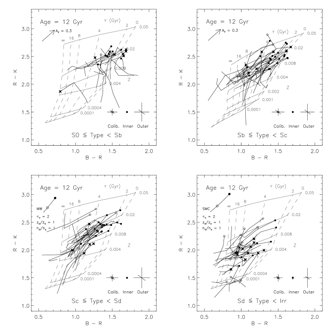
Figure 2: Trends in optical–near-IR colour with morphological type. We plot $B-R$ against $R-K$ colours for those galaxies with photometry in $B$, $R$ and $K$ (92 per cent of the sample; solid lines). Central colours are denoted by solid circles (for the sample from dJiv), open circles (for the sample from Paper i) or stars (for the sample from TVPHW). Overplotted are the KA97 (upper right panel) and BC98 (remaining panels) stellar population models. Note that the lower right panel is labelled with the average age of the stellar population $\langle A\rangle$; the remaining panels are labelled with the star formation timescale $\tau$. We also show the calibration uncertainties and the sky subtraction uncertainties in the inner and outer annuli: the diagonal lines in these error bars represent the effect of a 1$\sigma$ shift in the $R$ band photometry. Overplotted also are the foreground screen (upper panels) and Triplex model (lower panels) dust models. In the Triplex model, the solid circle denotes the central reddening, and the open circle the reddening at the half light radius. Further discussion of the data and model grids is undertaken in the text.

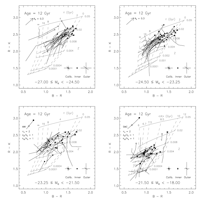
Figure 3: Trends in optical–near-IR colour with $K$ band magnitude. The symbols are as in Fig. 2. The two sets of colours for UGC 334 from dJiv and Paper i are also shown, connected by a dotted line.

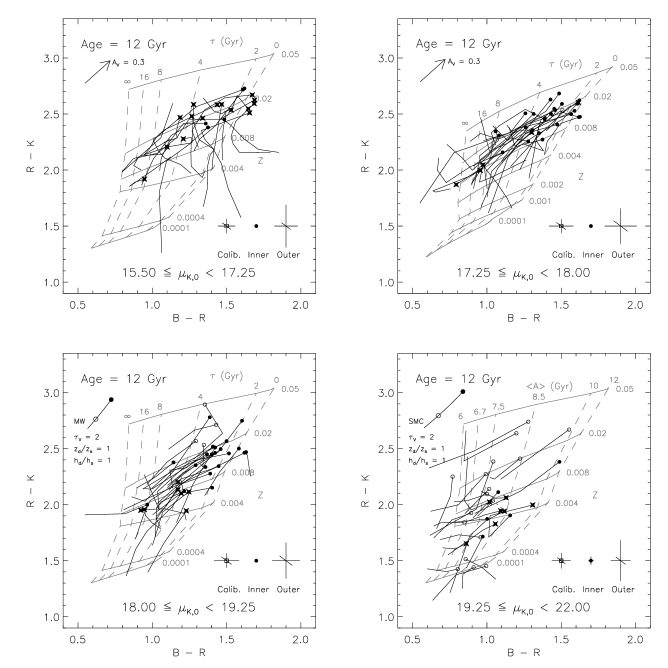
Figure 4: Trends in optical–near-IR colour with $K$ band central surface brightness. The symbols are as in Fig. 2. The two sets of colours for UGC 334 from dJiv and Paper i are also shown, connected by a dotted line.

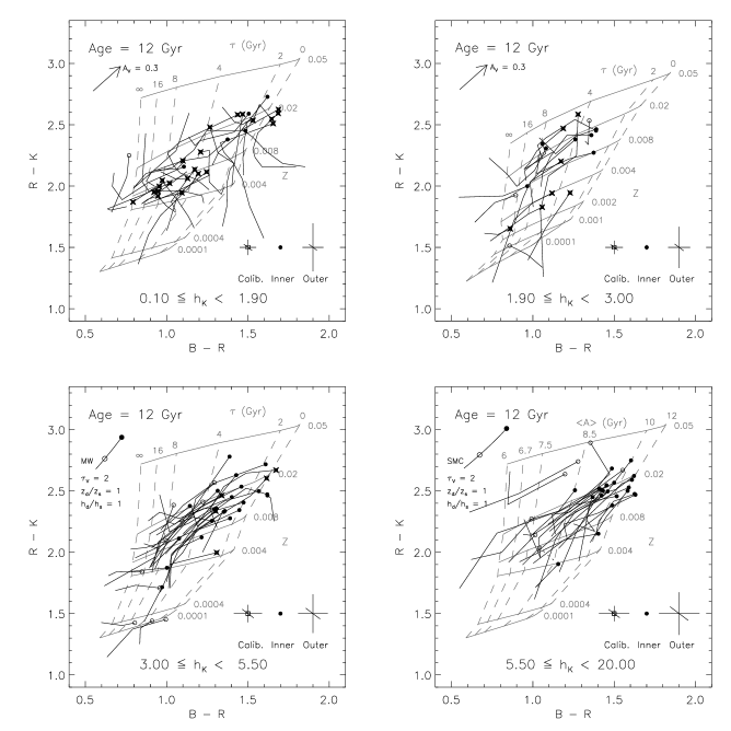
Figure 5: Trends in optical–near-IR colour with $K$ band disc scale length in kpc. The symbols are as in Fig. 2. The two sets of colours for UGC 334 from dJiv and Paper i are also shown, connected by a dotted line.

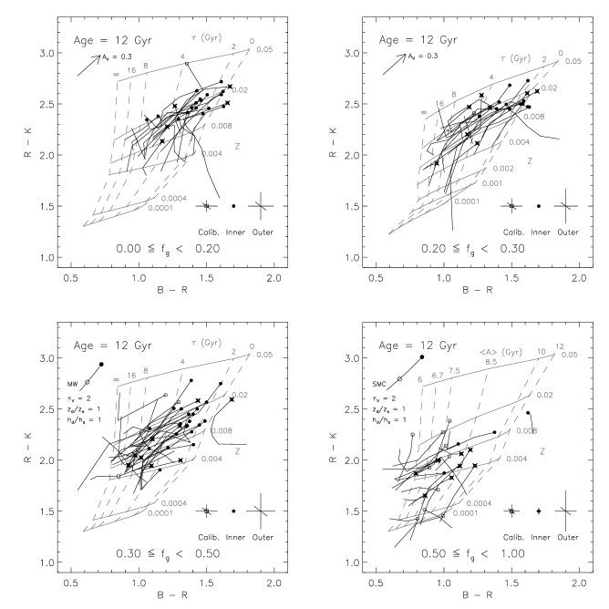
Figure 6: Trends in optical–near-IR colour with gas fraction. The symbols are as in Fig. 2.

In order to gain insight into age and metallicity trends as a function of radius, we perform a weighted linear fit to the ages and metallicities of each galaxy. This fit is parameterised by a gradient per disc scale length and an intercept at the disc half light radius.

Each point entering the fit is weighted by the total age or metallicity error in each annulus, determined using $\Delta\chi^{2}=1$ intervals for the age and metallicity parameters individually (i.e. the age or metallicity range for which the reduced $\chi^{2}$ is smaller than $\chi_{\rm best\,fit}^{2}+1$). The first two, three or four bins of the radially-resolved ages and metallicities are used in the fit. Galaxies with only central colours are omitted from the sample, and galaxies with more than four bins are fit only out to the fourth bin. Including the fifth, sixth and seventh bins in the gradient fits does not significantly affect our results, but can increase the noise in the gradient determinations.

As two out of the three sources of photometric error are correlated over the galaxy, it is impossible to use the $\Delta\chi^{2}=1$ contours for each annulus to estimate e.g. the errors in age and metallicity gradients. This is because to a large extent calibration uncertainties will not affect the age or metallicity gradient; however, the errors for the age or metallicity intercept will depend sensitively on the size of calibration error. We, therefore, produce error estimates using a Monte Carlo approach.

For each galaxy, we repeat the above SFH derivation and analysis 100 times, applying a normally distributed random calibration, flat fielding and sky level errors. This approach has the virtue that the different types of photometric error act on the galaxy profile as they should, allowing valid assessment of the accuracy of any trends in age or metallicity with radius. An example of the ages and metallicities derived with this approach for the galaxy UGC 3080 is presented in Fig. 1. The solid line indicates the best-fit model for the galaxy colours as a function of radius, and the dotted lines the Monte Carlo simulations with realistic (or perhaps slightly conservative) photometric errors. Note that the errors in age and metallicity increase substantially with radius. This is primarily due to the sky subtraction errors, as their effect increases as the surface brightness becomes fainter with radius. Note that because we use a weighted fit, the age and metallicity gradients are robust to the largest of the sky subtraction errors in the outer parts.

The error in any one parameter, e.g. metallicity, in any one annulus is given by the half of the interval containing 68 per cent of the e.g. metallicities in that annulus (the one sigma confidence interval). Errors in the age or metallicity gradients and intercepts are determined by fitting the 100 Monte Carlo simulated datasets in the same way as the real data. As above, the errors in each of these fit parameters are determined by working out the one sigma confidence interval of the simulations for each fit parameter alone.

4 Results

4.1 Colour-colour plots

In order to better appreciate the characteristics of the data, the model uncertainties and the potential effects of dust reddening on the results, it is useful to consider some colour-colour plots in some detail. In Figs. 2 through 6 we show $B-R$ against $R-K$ colours as a function of radius for our sample galaxies. Central colours are denoted by solid circles (for the sample from dJiv), open circles (for the sample from Paper i) or stars (for the sample from TVPHW). Overplotted is the SPS model of KA97 in the upper right panel; in the remaining panels we plot BC98’s model. Note that the lower right panel is labelled with the average age of the stellar population $\langle A\rangle$; the remaining panels are labelled with the star formation timescale $\tau$. In the upper panels we show a dust reddening vector assuming that dust is distributed in a foreground screen, and in the lower panels we show two absorption reddening vectors from the analytical treatment of DDP and Evans [Evans 1994].

These figures clearly reiterate the conclusions of Paper i and dJiv, where it was found that colour gradients were common in all types of spiral discs. Furthermore, these colour gradients are, for the most part, consistent with gradients in mean stellar age. The effects of dust reddening may also play a rôle; however, dust is unlikely to produce such a large colour gradient: see section 5.4 and e.g. Kuchinski et al. [Kuchinski et al. 1998] for a more detailed justification.

A notable exception to this trend are the relatively faint S0 galaxies from the sample of TVPHW (see Fig. 2). These galaxies show a strong metallicity gradient, and an inverse age gradient, in that the outer regions of the galaxy appear older and more metal poor than the younger and more metal rich central regions of the galaxy. This conclusion is consistent with the results from studies of line strength gradients: Kuntschner [Kuntschner 1998] finds that many of the fainter S0s in his sample have a relatively young and metal rich nucleus, with older and more metal poor outer regions.

Also, in Fig. 2, we find that there is a type dependence in the galaxy age and metallicity, in the sense that later type galaxies are both younger and more metal poor than their earlier type counterparts. This is partially consistent with dJiv, who finds that later type spirals have predominantly lower stellar metallicity (but he finds no significant trends in mean age with galaxy type).

In Figs. 3 to 6 we explore the differences in SFH as a function of the physical parameters of our sample galaxies. Figure 5 suggests there is little correlation between galaxy scale length and SFH: there may be a weak correlation in the sense that there are very few young and metal poor large scale length galaxies. In contrast, when taken together, Figs. 3, 4 and 6 suggest that there are real correlations between the SFHs of spiral galaxies (as probed by the ages and metallicities) and the magnitudes, central surface brightnesses and gas fractions of galaxies in the sense that brighter, higher surface brightness galaxies with lower gas fractions tend to be older and more metal rich than fainter, lower surface brightness galaxies with larger gas fractions. Later, we will see these trends more clearly in terms of average ages and metallicities, but it is useful to bear in mind these colour-colour plots when considering the trends presented in the remainder of this section.

4.2 Local ages and metallicities

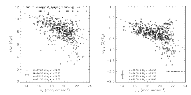
Figure 7: Local average age (left) and metallicity (right) against $K$ band surface brightness. The average age $\langle A\rangle$ and metallicity $\log_{10}(Z/Z_{\sun})$ of each galaxy annulus is shown against the local average $K$ band surface brightness $\mu_{K}$. The galaxies are binned by $K$ band absolute magnitude: note that this binning clearly shows the magnitude dependence in the local metallicity–surface brightness correlation. The dashed lines are unweighted least-squares fits to the data: the fits and significances are given in Table 1. A significant number of data points have average ages of 11.9 Gyr or metallicities of $\log_{10}(Z/Z_{\sun})=-2$: these data points fall outside the model grids.

We investigate the relation between the average ages and metallicities inferred from the colours of each galaxy annulus and the average $K$ band surface brightness in that annulus in Fig. 7. Representative error bars from the Monte Carlo simulations are shown in the lower left hand corner of the plots. Strong, statistically significant correlations between local age and the $K$ band surface brightness, and between local metallicity and the $K$ band surface brightness are found. While the scatter is considerable, the existence of such a strong relationship between local $K$ band surface brightness and the age and metallicity in that region is remarkable. In order to probe the dependence of the SFH on the structural parameters of our sample, we have carried out unweighted least-squares fits of these and subsequent correlations: the results of these fits are outlined in Table 1. In Table 1 we give the coefficients of the unweighted least-squares fits to the correlations significant at the 99 per cent level (where the significances are determined from a Spearman rank order test), along with errors derived from bootstrap resampling of the data [Press et al. 1986]. We will address these correlations further in the next section and in the discussion (section 5), where we attempt to relate these strong local correlations with global correlations.

4.3 Global relations

Figure 8: Correlations between the average age $\langle A\rangle_{eff}$ at the disc half light radius and the $K$ band central surface brightness $\mu_{K,0}$, $K$ band absolute magnitude $M_{K}$, $K$ band disc scale length $h_{K}$ and gas fraction $f_{g}$ (see text for the details of the derivation of the gas fractions). In this and subsequent figures error bars denote the estimated 68 per cent confidence intervals, and dashed lines are unweighted least-squares fits to trends significant at greater than the 99 per cent level (see Table 1). The solid lines in the top two panels denote the unweighted least-squares fit to the age–magnitude–surface brightness correlation, projected onto the age–surface brightness and age–magnitude planes.

Figure 9: Correlations between the average metallicity $\log_{10}(Z_{eff}/Z_{\sun})$ at the disc half light radius and $K$ band central surface brightness, $K$ band absolute magnitude, $K$ band disc scale length and gas fraction. Dashed lines are unweighted least-squares fits to trends significant at greater than the 99 per cent level (see Table 1). The solid lines in the top two panels denote the unweighted least-squares fit to the metallicity–magnitude–surface brightness correlation, projected onto the metallicity–surface brightness and metallicity–magnitude planes. The solid line in the lower right panel shows the expectation for the mean stellar metallicity with gas fraction for a closed-box model with a solar metallicity yield.

Figure 10: Correlations between the average age gradient per $K$ band disc scale length ($d\langle A\rangle/dr$) and the $K$ band central surface brightness, $K$ band absolute magnitude, $K$ band disc scale length and the gas fraction. Dashed lines are unweighted least-squares fits to trends significant at greater than the 99 per cent level (see Table 1).

Figure 11: Correlations between the average metallicity gradient $d{\log_{10}(Z_{eff}/Z_{\sun})}/dr$ in terms of the $K$ band disc scale length $h_{K}$ and the $K$ band central surface brightness, $K$ band absolute magnitude, $K$ band disc scale length and gas fraction.

Figure 12: Correlation between $K$ magnitudes, $K$ band central surface brightnesses, $K$ band disc scale lengths and gas fractions. Correlations between the physical parameters are important to bear in mind when interpreting the correlations in Figs. 8–11. The solid line in the upper left panel is the unweighted least-squares bisector fit to the magnitude–central surface brightness correlation. The solid line in the lower left panel is the estimated fit to the gas fraction–magnitude relation (see section 5.5).

In addition to the individual annulus age and metallicity estimates, we calculated age and metallicity best-fit gradients and intercepts (as described in section 3.1). These fit parameters are useful, in that they allow us to probe the global relationships between e.g. magnitude and SFH.

These fits to an individual galaxy are parameterised by their gradient (in terms of the inverse $K$ band scale lengths) and their intercept (expressed as the intercept at the disc half light radius $R_{eff}$). We explore correlations between the structural parameters and the radial age and metallicity fit parameters in Figs. 8–11.

4.3.1 Global ages

In Fig. 8, we see how the age intercept at the half light radius relates to the $K$ band surface brightness, $K$ band absolute magnitude, $K$ band disc scale length and gas fraction.

As expected from the strong correlation between the local surface brightness and age, there is a highly significant correlation between the $K$ band central surface brightness and age. We see also that there are also highly significant correlations between the $K$ band absolute magnitude and age, and the gas fraction and age. There is no significant correlation between age and $K$ band disc scale length.

An important question to ask at this stage is: are these correlations related to each other in some way? We investigate this in Fig. 12, where we plot some of the physical parameters against each other. We see that the $K$ band absolute magnitude of this sample is correlated (with large scatter) with the $K$ band central surface brightness. We also see in Fig. 12 that the brightest galaxies all have the largest scale lengths. In addition, both magnitude and surface brightness correlate strongly with the gas fraction. From these correlations, we can see that all of the three correlations between age and central surface brightness, magnitude and gas fraction may have a common origin: the correlation between these three physical parameters means that it is difficult, using Fig. 8 alone, to determine which parameters age is sensitive to. We do feel, however, that the correlations between age and surface brightness and age and magnitude do not stem from the correlation between age and gas fraction for two reasons. Firstly, the scatter in the age–gas fraction relationship is comparable to or even larger than the age–surface brightness and age–magnitude correlations. Secondly, the gas fraction is an indication of the total amount of star formation over the history of a galaxy (assuming that there is little late gas infall), implying that the gas fraction is quite dependent on the SFH. Therefore, correlations between SFH and gas fraction are likely to be driven by this effect, rather than indicating that gas fraction drives SFH.

To summarise Figs. 8 and 12, the age of a galaxy is correlated strongly with the $K$ band surface brightness, $K$ band absolute magnitude and the gas fraction. We discuss these important correlations further in section 5.1.

4.3.2 Global metallicities

In Fig. 9, we see how the metallicity intercept at the disc half light radius relates to the $K$ band surface brightness, $K$ band absolute magnitude, $K$ band disc scale length and gas fraction.

The trends shown in Fig. 9 are similar to those seen in Fig. 8: this demonstrates the close correlation between the age and metallicity of a galaxy, in the sense that older galaxies are typically much more metal rich than their younger brethren. However, there are some important differences between the two sets of correlations.

Firstly, although the correlation is not statistically significant, there is a conspicuous lack of galaxies with large scale lengths and low metallicities. This lack of large, metal poor galaxies can be understood from the relationship between magnitude and scale length in Fig. 12: large galaxies, because of their size, are bright by default (even if they have low surface brightnesses; Paper i) and have near-solar metallicities.

Secondly, there seems to be a kind of ‘saturation’ in the stellar metallicities that was not apparent for the mean ages. It is particularly apparent in the correlation between the metallicity and $K$ band absolute magnitude: the metallicity of galaxies with an absolute $K$ band magnitude of $-22$ is very similar to the metallicity of galaxies that are nearly 40 times brighter, with an absolute $K$ band magnitude of $-26$. The metallicity of galaxies fainter than an absolute $K$ band magnitude of $-22$ can be much lower, to the point where the metallicities are too low to be included reliably on the stellar population model grid. This ‘saturation’ is easily understood in terms of the gas fractions: the near-solar metallicity galaxies tend to have gas fractions $\la$ 0.5. In this case, assuming a closed box model of chemical evolution (i.e. no gas flows into or out of the galaxy, and the metals in the galaxy are well-mixed), the stellar metallicity will be within 0.5 dex of the yield (see Pagel 1998 and references therein), which in this case would indicate a yield around, or just above, solar metallicity. This case is shown in the lower right panel of Fig. 9 (also Fig. 16), where we show the stellar metallicity of a solar metallicity yield closed box model against the gas fraction. Note that the gas metallicity in the closed box model continues to rise to very low gas fractions: this will become important later when we compare the stellar metallicity–luminosity relation from this work with the gas metallicity–luminosity relation (section 5.5).

4.3.3 Age gradients

Figure 13: Correlations between galaxy type and age gradient. The x-axis is the T-type, where types between $-3$ and $-0$ correspond to S0s, and types 1 through 10 correspond to a smooth sequence from Sa to Im. The dashed line is the unweighted least-squares fit to the data.

In Fig. 10, we see how the age gradient (per $K$ band disc scale length) relates to the $K$ band surface brightness, $K$ band absolute magnitude, $K$ band disc scale length and gas fraction.

An important first result is that, on average, we have a strong detection of an overall age gradient: the average age gradient per $K$ band disc scale length is $-0.79\pm 0.08$ Gyr $h^{-1}$ (10$\sigma$; where the quoted error is the error in the mean gradient).

We see that the age gradient does not correlate with the $K$ band absolute magnitude. However, there are statistically significant correlations between the age gradient and $K$ band central surface brightness, $K$ band disc scale length and gas fraction. Smaller galaxies, higher surface brightness galaxies and low gas fraction galaxies all tend to have relatively flat age gradients (with much scatter, that almost exceeds the amplitude of the trend).

One possibility is that the S0s with ‘inverse’ age gradients (in the sense that their central regions were younger than their outer regions) are producing these trends, as the S0s in this sample are relatively faint (therefore not producing much of a trend in age gradient with magnitude) but have high surface brightness, small sizes and low gas fractions (therefore producing trends in all of the other physical parameters).

We investigate this possibility in Fig. 13. Here we see that the trend is not simply due to ‘contamination’ from a small population of S0s: S0s contribute to a more general trend of decreasing age gradients for earlier galaxy types. Therefore, this decrease in age gradient is a real effect. We address a possible cause for this phenomenon later in section 5.6.

4.3.4 Metallicity gradients

In Fig. 11, we see how the metallicity gradient (per $K$ band disc scale length) relates to the $K$ band surface brightness, $K$ band absolute magnitude, $K$ band disc scale length and gas fraction. The metallicity gradient is fairly poorly determined because of its typically smaller amplitude, and sensitivity to the rather noisier near-IR colours. Also, because of its smaller amplitude, metallicity gradients are more susceptible to the effects of dust reddening than were the rather larger age gradients. On average (assuming that the effects of dust are negligible), we have detected an overall metallicity gradient (although with much scatter): the average metallicity gradient per $K$ band disc scale length is $-0.14\pm 0.02$ dex $h^{-1}$ (7$\sigma$; where again the quoted error is the error in the mean gradient). Due to the large observational scatter, however, we have failed to detect any trends in metallicity gradient with galaxy properties.

Table 1: Unweighted least-squares fits for the statistically significant correlations (with significance $>$ 99 per cent) between SFH and galaxy structural parameters presented in Figs. 7–11 and 13–15.

X	Y	Slope		Intercept		$P^{a}$
$\mu_{K}$	$\langle A\rangle$ (Gyr)	$-$0.42$\pm$	0.04	8.20$\pm$	0.07	6.2$\times$	10-24
$\mu_{K}$	$\log_{10}(Z/Z_{\sun})$	$-$0.132$\pm$	0.011	$-$0.43$\pm$	0.03	2.4$\times$	10-30
$\mu_{K,0}$	$\langle A\rangle_{eff}$ (Gyr)	$-$0.81$\pm$	0.14	6.6$\pm$	0.3	2.9$\times$	10-10
$M_{K}$	$\langle A\rangle_{eff}$ (Gyr)	$-$0.38$\pm$	0.09	6.8$\pm$	0.3	2.3$\times$	10-6
$f_{g}$	$\langle A\rangle_{eff}$ (Gyr)	$-$4.8$\pm$	1.0	9.6$\pm$	0.3	4.1$\times$	10-10
$\mu_{K,0}$	$\log_{10}(Z_{eff}/Z_{\sun})$	$-$0.22$\pm$	0.04	$-$0.80$\pm$	0.09	4.9$\times$	10-8
$M_{K}$	$\log_{10}(Z_{eff}/Z_{\sun})$	$-$0.15$\pm$	0.02	$-$0.86$\pm$	0.09	2.6$\times$	10-9
$f_{g}$	$\log_{10}(Z_{eff}/Z_{\sun})$	$-$1.4$\pm$	0.3	0.12$\pm$	0.08	1.0$\times$	10-8
$\mu_{K,0}$	$d\langle A\rangle/dr$ (Gyr/$h$)	$-$0.25$\pm$	0.07	$-$1.2$\pm$	0.2	1.4$\times$	10-6
$\log_{10}(h_{K})$	$d\langle A\rangle/dr$ (Gyr/$h$)	$-$1.0$\pm$	0.3	$-$0.30$\pm$	0.15	1.2$\times$	10-6
$f_{g}$	$d\langle A\rangle/dr$ (Gyr/$h$)	$-$1.1$\pm$	0.5	$-$0.5$\pm$	0.2	4.5$\times$	10-4
Type	$d\langle A\rangle/dr$ (Gyr/$h$)	$-$0.08$\pm$	0.03	$-$0.38$\pm$	0.16	5.9$\times$	10-4
$M_{K}$	$\log_{10}(Z_{eff}/Z_{\sun})-\log_{10}(Z_{\mu}/Z_{\sun})$	-0.08$\pm$	0.02	-0.22$\pm$	0.07	1.9$\times$	10-4
$\mu_{K,0}$	$\langle A\rangle_{eff}-\langle A\rangle_{M}$ (Gyr)	-0.60$\pm$	0.15	-0.9$\pm$	0.3	1.3$\times$	10-6
$\mu_{K,0}$	$\log_{10}(Z_{eff}/Z_{\sun})-\log_{10}(Z_{M}/Z_{\sun})$	-0.13$\pm$	0.03	-0.22$\pm$	0.08	2.6$\times$	10-4
Modified $\mu_{K,0}$	$\langle A\rangle_{eff}$ (Gyr)	-0.9$\pm$	0.2	5.7$\pm$	0.5	1.1$\times$	10-7
Modified $M_{K}$	$\langle A\rangle_{eff}$ (Gyr)	-0.52$\pm$	0.09	6.0$\pm$	0.4	8.9$\times$	10-9
Modified $\mu_{K,0}$	$\log_{10}(Z_{eff}/Z_{\sun})$	-0.21$\pm$	0.05	-0.9$\pm$	0.1	4.9$\times$	10-6
Modified $M_{K}$	$\log_{10}(Z_{eff}/Z_{\sun})$	-0.14$\pm$	0.03	-0.9$\pm$	0.1	2.3$\times$	10-7

${}^{a}\,P$ is defined as the probability of the correlation being the result of random fluctuations in an uncorrelated dataset: the usual definition of significance is $(1-P)$.

Surface brightness intercepts are quoted at a $K$ band surface brightness of 20 mag arcsec^-2.

Absolute magnitude intercepts are quoted at a $K$ band absolute magnitude of $-20$.

5 Discussion

5.1 Surface brightness vs. magnitude

Figure 14: The top two panels show the residuals from the age–surface brightness correlation of Fig. 8 and the metallicity–surface brightness correlation of Fig. 9 against $K$ band absolute magnitude. The lower two panels show the residuals from the age–magnitude correlation of Fig. 8 and the metallicity–magnitude correlation of Fig. 9 against $K$ band central surface brightness. Dashed lines are unweighted least-squares fits to trends significant at greater than the 99 per cent level (see Table 1).

In the previous section, we presented a wide range of correlations between diagnostics of the SFH and the physical parameters that describe a spiral galaxy. Our main finding was that the SFH of a galaxy correlates well with both the $K$ band absolute magnitude and $K$ band surface brightness. However, this leaves us in an uncomfortable position: because of the surface brightness–magnitude correlation in our dataset (Fig. 12), it is impossible to tell from Figs. 8, 9 and 12 alone what parameter is more important in determining the SFH of a galaxy.

One straightforward way to investigate which parameter is more important is by checking if the offset of a galaxy from e.g. the age–magnitude correlation of Fig. 8 correlates with surface brightness.

In the upper panels of Fig. 14, we show the residuals from the age–surface brightness correlation and the metallicity–surface brightness correlation against magnitude. Age residual does not significantly correlate with magnitude (the correlation is significant at only the 97 per cent level and is not shown). Metallicity residuals are significantly correlated with the magnitude, where brighter galaxies tend to be more metal rich than expected from their surface brightness alone.

In the lower panels of Fig. 14, we show the residuals from the age–magnitude correlation and the metallicity–magnitude correlation. In contrast to the upper panels of this figure, there are highly significant correlations between the age residual and surface brightness, and the metallicity residual and surface brightness.

Another way to consider the above is to investigate the distribution of galaxies in the three dimensional age–magnitude–surface brightness and metallicity–magnitude–surface brightness spaces. Unweighted least-squares fits of the age and metallicity as a function of surface brightness and magnitude yield the surfaces:

$$\langle A\rangle_{eff} = 6.24(\pm 0.14)-0.71(\pm 0.06)(\mu_{K,0}-20)$$

$$-0.15(\pm 0.03)(M_{K}+20)$$

$$\log_{10}(Z_{eff}/Z_{\sun}) = -0.99(\pm 0.05)$$

$$-0.17(\pm 0.01)(\mu_{K,0}-20)$$

$$-0.10(\pm 0.01)(M_{K}+20),$$

where the quoted errors (in brackets) are derived using bootstrap resampling of the data and the intercept is defined at $\mu_{K,0}=20$ mag arcsec^-2 and $M_{K}=-20$. A best fit line to the dataset is shown in Figs. 8 and 9. This best fit line is defined by the intersection of the best-fit plane with the least-squares bisector fit (where each variable is treated equally in the fit; Isobe et al. 1990) of the magnitude–surface brightness correlation (Fig. 12): $M_{K}=-19.75+1.88(\mu_{K,0}-20)$. No plots of the distribution of galaxies in these three-dimensional spaces are shown: the two-dimensional projections of this space in Figs. 8, 9 and 12 are among the best projections of this three-dimensional space.

From the above fits, we can see quite clearly that age is primarily sensitive to central surface brightness: the change in average age per magnitude change in central surface brightness is much larger than change in age per magnitude change in luminosity. The stellar metallicity of a galaxy is sensitive to both surface brightness and magnitude: this is clear from the fairly comparable change in metallicity per magnitude change in surface brightness or luminosity.

We have also analysed the residuals from the age–local $K$ band surface brightness and metallicity–local $K$ band surface brightness correlations as a function of central $K$ band surface brightness and $K$ band absolute magnitude (Fig. 7). The age of an annulus in a galaxy primarily correlates with its local $K$ band surface brightness and correlates to a lesser extent with the galaxy’s $K$ band central surface brightness and magnitude. The metallicity of a galaxy annulus correlates equally well with both the local $K$ band surface brightness and total galaxy magnitude and only very weakly with the central $K$ band surface brightness. Thus, the results from the analysis of local ages and metallicities are consistent with the analysis of the global correlations: much (but not all) of the variation that was attributed to the central surface brightness in the global analysis is driven by the local surface brightness in the local analysis. However, note that it is impossible to tell whether it is the global correlations that drive the local correlations, or vice versa. The local $K$ band surface brightnesses (obviously) correlate with the central $K$ band surface brightnesses, meaning that it is practically impossible to disentangle the effects of local and global surface brightnesses.

However, there must be other factors at play in determining the SFH of spiral galaxies: the local and global age and metallicity residuals (once all the above trends have been removed) show a scatter around 1.4 times larger than the (typically quite generous) observational errors, indicating cosmic scatter equivalent to $\sim$ 1 Gyr in age and $\sim$ 0.2 dex in metallicity. This scatter is intrinsic to the galaxies themselves and must be explained in any model that hopes to accurately describe the driving forces behind the SFHs of spiral galaxies. However, note that some or all of this scatter may be due to the influence of small bursts of star formation on the colours of galaxies.

To summarise, $K$ band surface brightness (in either its local or global form) is the most important ‘predictor’ of the the SFH of a galaxy: the effects of $K$ band absolute magnitude modulate the overall trend defined by surface brightness. Furthermore, it is apparent that the metallicity of a galaxy depends more sensitively on its $K$ band magnitude than does the age: this point is discussed later in section 5.6. On top of these overall trends, there is an intrinsic scatter, indicating that the surface brightness and magnitude cannot be the only parameters describing the SFH of a galaxy.

5.2 Star formation histories in terms of masses and densities

Figure 15: Correlations between the average age and metallicity at the disc half light radius and the modified $K$ band central surface brightness and absolute magnitudes. The surface brightnesses and absolute magnitude are modified to approximate total baryonic densities and masses, by turning the gas fraction of the galaxies into stars with a $K$ band mass to light ratio of 0.6 $M_{\sun}/L_{\sun}$. Dashed lines are unweighted least-squares fits to trends significant at greater than the 99 per cent level (see Table 1).

In the above, we have seen how age and metallicity vary as a function of $K$ band surface brightness and $K$ band absolute magnitude. $K$ band stellar mass to light ratios are expected to be relatively insensitive to differences in stellar populations (compared to optical passbands; e.g. dJiv). Therefore, the variation of SFH with $K$ band surface brightness and absolute magnitude is likely to approximately represent variations in SFH with stellar surface density and stellar mass (especially over the dynamic range in surface brightness and magnitude considered in this paper).

However, these trends with $K$ band surface brightness and $K$ band absolute magnitude may not accurately represent the variation of SFH with total (baryonic) surface density or mass: in order to take that into account, we must somehow account for the gas fraction of the galaxy. Accordingly, we have constructed ‘modified’ $K$ band surface brightnesses and magnitudes by adding $2.5\log_{10}(1-f_{g})$. This correction, in essence, converts all of the gas fraction (both the measured atomic gas fraction, and the much more uncertain molecular gas fraction) into stars with a constant stellar mass to light ratio in $K$ band of 0.6 $M_{\sun}/L_{\sun}$.

In this correction, we make two main assumptions. Firstly, we assume a constant $K$ band stellar mass to light ratio of 0.6 $M_{\sun}/L_{\sun}$. This might not be such an inaccurate assumption: the $K$ band mass to light ratio is expected to be relatively robust to the presence of young stellar populations; however, our assumption of a constant $K$ band mass to light ratio is still a crude assumption and should be treated with caution. Note, however, that the relative trends in Fig. 15 are quite robust to changes in stellar mass to light ratio: as the stellar mass to light ratio increases, the modified magnitudes and surface brightnesses creep closer to their unmodified values asymptotically.

Secondly, the correction to the surface brightness implicitly assumes that the gas will turn into stars with the same spatial distribution as the present-day stellar component. This is quite a poor assumption as the gas distribution is usually much more extended than the stellar distribution: this would imply that the corrections to the central surface brightnesses are likely to be overestimates. However, our purpose here is not to construct accurate measures of the baryonic masses and densities of disc galaxies; our purpose is merely to try to construct some kind of representative mass and density which will allow us to determine if the trends in SFH with $K$ band magnitude and surface brightness reflect an underlying, more physically meaningful trend in SFH with mass and density.

In Fig. 15 we show the trends in age at the disc half light radius (left hand panels) and metallicity at the disc half light radius (right hand panels) with modified $K$ band central surface brightness (upper panels) and modified $K$ band magnitude (lower panels). It is clear that the trends in SFH with $K$ band surface brightness and absolute magnitude presented in Figs. 8 and 9 represent an underlying trend in SFH with the total baryonic galaxy densities and masses. The best fit slopes are typically slightly steeper than those for the unmodified magnitudes and surface brightnesses (Table 1): because low surface brightness and/or faint galaxies are gas-rich, correcting them for the contributions from their gas fractions tends to steepen the correlations somewhat. We have also attempted to disentangle surface density and mass dependencies in the SFH using the method described above in section 5.1: again, we find that surface density is the dominant parameter in determining the SFH of a galaxy, and that the mass of a galaxy has a secondary, modulating effect on the SFH.

5.3 Does the choice of IMF and SPS model affect our conclusions?

We have derived the above conclusions using a Salpeter [Salpeter 1955] IMF and the BC98 models, but are our conclusions affected by SPS model details such as IMF, or the choice of model? We address this possible source of systematic uncertainty in Table 2, where we compare the results for the correlation between the $K$ band central surface brightness $\mu_{K,0}$ and age intercept at the disc half light radius $\langle A\rangle_{eff}$ using the models of BC98 with the IMF adopted by Kennicutt [Kennicutt 1983] and the models of KA97 with a Salpeter IMF.

Table 2: Unweighted least-squares fits for the correlation between the $K$ band central surface brightness $\mu_{K,0}$ and age intercept at the half light radius $\langle A\rangle_{eff}$ using different SPS models and IMFs.

Model	IMF	Slope		Intercept		$P^{a}$
BC98	Salpeter	$-$0.81$\pm$	0.14	6.6$\pm$	0.3	2.9$\times$	10-10
BC98	Kennicutt	$-$0.93$\pm$	0.14	6.2$\pm$	0.3	3.3$\times$	10-10
KA97	Salpeter	$-$0.82$\pm$	0.12	6.1$\pm$	0.3	8.8$\times$	10-11

${}^{a}\,P$ is defined as the probability of the correlation being the result of random fluctuations in an uncorrelated dataset: the usual definition of significance is $(1-P)$.
The intercept is quoted at a $K$ band central surface brightness of 20 mag arcsec^-2.

From Table 2, it is apparent that our results are quite robust to changes in both the stellar IMF and SPS model used to interpret the data. In none of the cases does the significance of the correlation vary by a significant amount, and the slope and intercept of the correlation varies within its estimated bootstrap resampling errors. This correlation is not exceptional; other correlations show similar behaviour, with little variation for plausible changes in IMF and SPS model. In conclusion, while plausible changes in the IMF and SPS model will change the details of the correlations (e.g. the gradients, intercepts, significances, etc.), the existence of the correlations themselves is very robust to changes in the models used to derive the SFHs.

5.4 How important is dust extinction?

Our results account for average age and metallicity effects only; however, from Figs. 2–6 it is clear that dust reddening can cause colour changes similar to those caused by age or metallicity. In this section, we discuss the colour changes caused by dust reddening. We conclude that dust reddening will mainly affect the metallicity (and to a lesser extent age) gradients: however, the magnitude of dust effects is likely to be too small to significantly affect our conclusions.

In Figs. 2–6, we show the reddening vectors for two different dust models (Milky Way and Small Magellanic Cloud dust models) and for two different reddening geometries (a simple foreground screen model and exponential star and dust disc model). We can see that the reddening effects of the foreground screen (for a total $V$ band extinction of 0.3 mag) are qualitatively similar (despite its unphysical dust geometry) to the central $V$ band absorption of a $\tau_{V}=2$ Triplex dust model. For the Triplex model, the length of the vector shows the colour difference between the central (filled circle) and outer colours, and the open circle denotes the colour effects at the disc half light radius.

How realistic are these Triplex vectors? dJiv compares absorption-only face-on Triplex dust reddening vectors with the results of Monte Carlo simulations, including the effects of scattering, concluding that the Triplex model vectors are quite accurate for high optical depths but that they considerably overestimate the reddening for lower optical depths (i.e. $\tau_{V}\la 2$). However, both these models include only the effects of smoothly distributed dust. If a fraction of the dust is distributed in small, dense clumps, the reddening produced by a given overall dust mass decreases even more: the dense clumps of dust tend to simply ‘drill holes’ in the face-on galaxy light distribution, producing very little reddening per unit dust mass [Huizinga 1994, dJiv, Kuchinski et al. 1998]. The bottom line is that in such a situation, the galaxy colours are dominated by the least obscured stars, with the dense dust clouds having little effect on the overall colour. Therefore, the Triplex model vectors in Figs. 2–6 are arguably overestimates of the likely effects of dust reddening on our data.

From Figs. 2–6, we can see that the main effect of dust reddening would be the production of a colour gradient which would mimic small artificial age and metallicity gradients. Note, however, that the amplitudes of the majority of the observed colour gradients are larger than the Triplex model vectors. In addition, we have checked for trends in age and metallicity gradient with galaxy ellipticity: no significant trend was found, suggesting that age and metallicity trends are unlikely to be solely produced by dust. Coupled with the above arguments, this strongly suggests that most of the colour gradient of a given galaxy is likely to be due to stellar population differences. This is consistent with the findings of Kuchinski et al. [Kuchinski et al. 1998], who found, using more realistic dust models tuned to reproduce accurately the colour trends in high-inclination galaxies, that the colour gradients in face-on galaxies were likely to be due primarily to changes in the underlying stellar populations with radius. Therefore, our measurements of the age and metallicity gradients are likely to be qualitatively correct, but trends in dust extinction with e.g. magnitude or surface brightness may cause (or hide) weak trends in the gradients.

The age and metallicity intercepts at the half light radius would be relatively unaffected: in particular, differences between the central $V$ band optical depths of 10 or more cannot produce trends in the ages or metallicities with anywhere near the dynamic range observed in the data. Therefore, the main conclusion of this paper, that the SFH of a spiral galaxy is primarily driven by surface density and is modulated by mass, is robust to the effects of dust reddening.

5.5 Comparison with H ii region metallicities

Figure 16: Comparison between the trends in gas metallicity and magnitude and stellar metallicity and magnitude. Our data from Fig. 9 are overplotted on H ii region metallicity determinations at a radius of 3 kpc for the sample of Vila-Costas & Edmunds (1992; VCE) (diamonds) and Zaritsky et al. (1994; ZKH) (diagonal crosses). Global gas metallicity determinations for dwarf galaxies are taken from Skillman et al. (1989; SKH) (triangles) and van Zee et al. [van Zee et al. 1997] (squares). Multiple metallicity determinations for the same galaxy are connected by solid lines. The dashed and solid lines are the closed box predictions for the gas metallicity–magnitude and stellar metallicity–magnitude relations, respectively (see text for details).

In Fig. 16, we plot our colour-based stellar metallicities at the disc half light radius against measures of the global gas metallicity via H ii region spectroscopy. $B$ band magnitudes were transformed into $K$ band magnitudes using an average $B-K$ colour of $3.4\pm 0.4$ [dJiv]. For bright galaxies, we have plotted metallicity determinations from Vila-Costas & Edmunds [Vila-Costas & Edmunds 1992] (diamonds) and Zaritsky et al. [Zaritsky, Kennicutt & Huchra 1994] (diagonal crosses) at a fixed radius of 3 kpc. To increase our dynamic range in terms of galaxy magnitude, we have added global gas metallicity measures from the studies of Skillman et al. [Skillman, Kennicutt & Hodge 1989] and van Zee et al. [van Zee et al. 1997]. Measurements for the same galaxies in different studies are connected by solid lines.

From Fig. 16, it is clear that our colour-based stellar metallicities are in broad agreement with the trends in gas metallicity with magnitude explored by the above H ii region studies. However, there are two notable differences between the colour-based stellar metallicities and the H ii region metallicities.

Firstly, there is a ‘saturation’ in stellar metallicity at bright magnitudes not seen in the gas metallicities, which continue to rise to the brightest magnitudes. In section 4.3.2, we argued that this ‘saturation’ was due to the slow variation of stellar metallicity with gas fraction at gas fractions lower than $\sim$ 1/2. In Fig. 16 we test this idea. The dashed line is the gas metallicity–magnitude relation expected if galaxies evolve as closed boxes with solar metallicity yield, converting between gas fraction and magnitude using the by-eye fit to the magnitude–gas fraction correlation $f_{g}=0.8+0.14(M_{K}-20)$ (where the gas fraction $f_{g}$ is not allowed to drop below 0.05 or rise above 0.95; see Fig. 12). The solid line is the corresponding relation for the stellar metallicity. Note that at $K$ band absolute magnitudes brighter than $-$25 or fainter than $-$19 the model metallicity–magnitude relation is poorly constrained: the gas fractions at the bright and faint end asymptotically approach zero and unity respectively. The closed box model indicates that our interpretation of the offset between gas and stellar metallicities at the brightest magnitudes is essentially correct: the gas metallicity of galaxies is around 0.4 dex higher than the average stellar metallicity. Furthermore, the slope of the gas metallicity–magnitude relation is slightly steeper than the stellar metallicity–magnitude relation. However, the simple closed box model is far from perfect: this model underpredicts the stellar metallicity of spiral galaxies with $K\sim-21$. This may be a genuine shortcoming of the closed box model; however, note that we have crudely translated gas fraction into magnitude: the closed box model agrees with observations quite closely if we plot gas and stellar metallicity against gas fraction (Fig. 9).

Secondly, there is a sharp drop in the estimated stellar metallicity at faint magnitudes that is not apparent in the gas metallicities. This drop, which occurs for stellar metallicities lower than $\sim 1/10$ solar, is unlikely to be physical: stellar and gas metallicities should be quite similar at high gas fractions (equivalent to faint magnitudes; Fig. 16). However, the SPS models are quite uncertain at such low metallicities, suggesting that the SPS models overpredict the near-IR magnitudes of very metal-poor composite stellar populations.

We have also compared our derived metallicity gradients with the gas metallicity gradients from Vila-Costas & Edmunds [Vila-Costas & Edmunds 1992] and Zaritsky et al. [Zaritsky, Kennicutt & Huchra 1994]. Though our measurements have large scatter, we detect an average metallicity gradient of $-0.06\pm 0.01$ kpc^-1 for the whole sample. This gradient is quite comparable to the average metallicity gradient from the studies Vila-Costas & Edmunds [Vila-Costas & Edmunds 1992] and Zaritsky et al. [Zaritsky, Kennicutt & Huchra 1994] of $-0.065\pm 0.007$ kpc^-1. Given the simplicity of the assumptions going into the colour-based analysis, and considerable SPS model and dust reddening uncertainties, we take the broad agreement between the gas and stellar metallicities as an important confirmation of the overall validity of the colour-based method.

5.6 A possible physical interpretation

Figure 17: Local average age (left), gas fraction (middle) and metallicity (right) against $K$ band surface brightness. The lines are predictions of the local density dependent model presented in the text with $n=1.4,k=0.020$ (dotted), $n=1.6,k=0.007$ (solid) and $n=1.8,k=0.0025$ (dashed).

In order to demonstrate the utility of the trends presented in section 4 in investigating star formation laws and galaxy evolution, we consider a simple model of galaxy evolution. We have found that the surface density of a galaxy is the most important parameter in describing its SFH; therefore, we consider a simple model where the star formation and chemical enrichment history are controlled by the surface density of gas in a given region [Schmidt 1959, Phillipps, Edmunds & Davies 1990, Phillipps & Edmunds 1991, Dopita & Ryder 1994, Elmegreen & Parravano 1994, Prantzos & Silk 1998, Kennicutt 1998]. In our model, we assume that the initial state 12 Gyr ago is a thin layer of gas with a given surface density $\sigma_{g}$. We allow this layer of gas to form stars according to a Schmidt [Schmidt 1959] star formation law:

$$\Psi(t)=-\frac{1}{\alpha}\frac{d\sigma_{g}(t)}{dt}=k\sigma_{g}(t)^{n},$$ (8)

where $\Psi(t)$ is the SFR at a time $t$, $\alpha$ is the fraction of gas that is locked up in long-lived stars (we assume $\alpha=0.7$ hereafter; this value is appropriate for a Salpeter IMF), $k$ is the efficiency of star formation and the exponent $n$ determines how sensitively the star formation rate depends on the gas surface density [Phillipps & Edmunds 1991]. Integration of Equation 8 gives:

$$\sigma_{g}(t)/\sigma_{0}=e^{-\alpha kt},$$ (9)

for $n=1$ and:

$$\sigma_{g}(t)/\sigma_{0}=[(n-1)\sigma_{0}^{n-1}\alpha kt+1]^{1/1-n},$$ (10)

for $n\neq 1$ where $\sigma_{0}$ is the initial surface density of gas. Note that the star formation (and gas depletion) history of the $n=1$ case is independent of initial surface density. To be consistent with the trends in SFH with surface brightness presented in this paper $n$ must be larger than one.

We allow no gas inflow or outflow from this region, i.e. our model is a closed box. In addition, in keeping with our definition of the star formation law above (where we allow a fraction of the gas consumed in star formation to be returned immediately, enriched with heavy elements), we use the instantaneous recycling approximation. While this clearly will introduce some inaccuracy into our model predictions, given the simplicity of this model a more sophisticated approach is not warranted. Using these approximations, it is possible to relate the stellar metallicity $Z$ to the gas fraction $f_{g}$ (e.g. Pagel & Pratchett 1975; Phillips & Edmunds 1991; Pagel 1998):

$$Z(t)=p(1+\frac{f_{g}\log f_{g}}{1-f_{g}}),$$ (11)

where $p$ is the yield, in this case fixed at solar metallicity $p=0.02$. Numerical integration of the SFR from Equations 8, 9 and 10 allows determination of the average age of the stellar population $\langle A\rangle$.

In modelling the SFH in this way, we are attempting to describe the broad strokes of the trends in SFH observed in Fig. 7, using the variation in SFH caused by variations in initial surface density alone. In order to meaningfully compare the models to the data, however, it is necessary to translate the initial surface density into a surface brightness. This is achieved using the solar metallicity SPS models of BC98 to translate the model SFR into a $K$ band surface brightness. While the use of the solar metallicity model ignores the effects of metallicity in determining the $K$ band surface brightness, the uncertainties in the $K$ band model mass to light ratio are sufficiently large that tracking the metallicity evolution of the $K$ band surface brightness is unwarranted for our purposes.

Using the above models, we tried to reproduce the trends in Fig. 7 by adjusting the values of $n$ and $k$. We found that reasonably good fits to both trends are easily achieved by balancing off changes in $n$ against compensating changes in $k$ over quite a broad range in $n$ and $k$. In order to improve this situation, we used the correlation between $K$ band central surface brightness and gas fraction as an additional constraint: in order to predict the relationship between central surface brightness and global gas fraction, we constructed the mass-weighted gas fraction for an exponential disc galaxy with the appropriate $K$ band central surface brightness. We found that models with $n\sim 1.6$ and $k\sim 0.007$ fit the observed trends well, with modest increases in $n$ being made possible by decreasing $k$, and vice versa. Plots of the fits to the age, metallicity and gas fraction trends with surface brightness are given in Fig. 17.

The success of this simple, local density-dependent model in reproducing the broad trends observed in Fig. 17 is quite compelling, re-affirming our assertion that surface density plays a dominant rôle in driving the SFH and chemical enrichment history of spiral galaxies. This simple model also explains the origin of age and metallicity gradients in spiral galaxies: the local surface density in spiral galaxies decreases with radius, leading to younger ages and lower metallicities at larger radii. Indeed, the simple model even explains the trend in age gradient with surface brightness: high surface brightness galaxies will have a smaller age gradient per disc scale length because of the flatter slope of the (curved) age–surface brightness relation at high surface brightnesses.

However, our simple model is clearly inadequate: there is no explicit mass dependence in this model, which is required by the data. This may be alleviated by the use of a different star formation law. Kennicutt [Kennicutt 1998] studied the correlation between global gas surface density and SFR, finding that a Schmidt law with exponent 1.5 or a star formation law which depends on both local gas surface density and the dynamical timescale (which depends primarily on the rotation curve shape, and, therefore, on mostly global parameters) explained the data equally well. There may also be a surface density threshold below which star formation cannot occur [Kennicutt 1989]. In addition, the fact that galaxy metallicity depends on magnitude and surface brightness in almost equal amounts (age is much more sensitive to surface brightness) suggests that e.g. galaxy mass-dependent feedback may be an important process in the chemical evolution of galaxies. Moreover, a closed box chemical evolution model is strongly disfavoured by e.g. studies of the metallicity distribution of stars in the Milky Way, where closed box models hugely overpredict the number of low-metallicity stars in the solar neighbourhood and other, nearby galaxies [Worthey, Dorman & Jones 1996, Pagel 1998]. This discrepancy can be solved by allowing gas to flow in and out of a region, and indeed this is expected in galaxy formation and evolution models set in the context of large scale structure formation [Cole et al. 1994, Kauffmann & Charlot 1998, Valageas & Schaeffer 1999].

6 Conclusions

We have used a diverse sample of low-inclination spiral galaxies with radially-resolved optical and near-IR photometry to investigate trends in SFH with radius, as a function of galaxy structural parameters. A maximum-likelihood analysis was performed, comparing SPS model colours with those of our sample galaxies, allowing use of all of the available colour information. Uncertainties in the assumed grid of SFHs, the SPS models and uncertainties due to dust reddening were not taken into account. Because of these uncertainties, the absolute ages and metallicities we derived may be inaccurate; however, our conclusions will be robust in a relative sense. In particular, dust will mainly affect the age and metallicity gradients; however, the majority of a given galaxy’s age or metallicity gradient is likely to be due to gradients in its stellar population alone. The global age and metallicity trends are robust to the effects of dust reddening. Our main conclusions are as follows.

• Most spiral galaxies have stellar population gradients, in the sense that their inner regions are older and more metal rich than their outer regions. The amplitude of age gradients increase from high surface brightness to low surface brightness galaxies. An exception to this trend are faint S0s from the Ursa Major Cluster of galaxies: the central stellar populations of these galaxies are younger and more metal rich than the outer regions of these galaxies.

• The stellar metallicity–magnitude relation ‘saturates’ for the brightest galaxies. This ‘saturation’ is a real effect: as the gas is depleted in the brightest galaxies, the gas metallicity tends to rise continually, while the stellar metallicity flattens off as the metallicity tends towards the yield. The colour-based metallicities of the faintest spirals fall considerably ($\ga 1$ dex) below the gas metallicity–luminosity relation: this may indicate that the SPS models overpredict the $K$ band luminosity of very low metallicity composite stellar populations.

• There is a strong correlation between the SFH of a galaxy (as probed by its age, metallicity and gas fraction) and the $K$ band surface brightness and magnitude of that galaxy. From consideration of the distribution of galaxies in the age–magnitude–surface brightness and metallicity–magnitude–surface brightness spaces, we find that the SFH of a galaxy correlates primarily with either its local or global $K$ band surface brightness: the effects of $K$ band absolute magnitude are of secondary importance.

• When the gas fraction is taken into account, the correlation between SFH and surface density remains, with a small amount of mass dependence. Motivated by the strong correlation between SFH and surface density, and by the correlation between age and local $K$ band surface brightness, we tested the observations against a closed box local density-dependent star formation law. We found that despite its simplicity, many of the correlations could be reproduced by this model, indicating that the local surface density is the most important parameter in shaping the SFH of a given region in a galaxy. A particularly significant shortcoming of this model is the lack of a magnitude dependence for the stellar metallicity: this magnitude dependence may indicate that mass-dependent feedback is an important process in shaping the chemical evolution of a galaxy. However, there is significant cosmic scatter in these correlations (some of which may be due to small bursts of recent star formation), suggesting that the mass and density of a galaxy may not be the only parameters affecting its SFH.

References

- [Abraham et al. 1998] Abraham R. G., Ellis R. S., Fabian A. C., Tanvir N. R., Glazebrook K., 1999, MNRAS, 303, 641
- [Allen 1973] Allen C. W., 1973, “Astrophysical Quantities”, University of London, The Athlone Press
- [Paper i] Bell E. F., Barnaby D., Bower R. G., de Jong R. S., Harper, Jr. D. A., Hereld M., Loewenstein R. F., Rauscher B. J., 1999, submitted to MNRAS (Paper i)
- [Bower, Lucey & Ellis 1992] Bower R. G., Lucey J. R., Ellis R. S., 1992, MNRAS, 254, 601
- [Bower, Kodama & Terlevich 1998] Bower R. G., Kodama, T., Terlevich A., 1998, MNRAS, 299, 1193
- [Bruzual & Charlot 1993] Bruzual A. G., Charlot S., 1993, ApJ, 405, 538
- [Bruzual, Magris & Calvet 1988] Bruzual A. G., Magris G., Calvet N., 1988, ApJ, 333, 673
- [Charlot, Worthey & Bressan 1996] Charlot S., Worthey G., Bressan A., 1996, ApJ, 457, 625
- [Cole et al. 1994] Cole S., Aragon-Salamanca A., Frenk C. S., Navarro J. F., Zepf S. E., 1994, MNRAS, 271, 781
- [de Blok, van der Hulst & Bothun 1995] de Blok W. J. G., van der Hulst J. M., Bothun G. D., 1995, MNRAS, 274, 235
- [de Blok, McGaugh & van der Hulst 1996] de Blok W. J. G., McGaugh S. S., van der Hulst J. M., 1996, MNRAS, 283, 18
- [dJii] de Jong R. S., 1996a, A&AS, 118, 557 (dJii)
- [de Jong 1996b] de Jong R. S., 1996b, A&A, 313, 45
- [dJiv] de Jong R. S., 1996c, A&A, 313, 377 (dJiv)
- [dJi] de Jong R. S., van der Kruit P. C., 1994, A&AS, 106, 451 (dJi)
- [DDP] Disney M. J., Davies J. I., Phillipps S., 1989, MNRAS, 239, 939 (DDP)
- [Dopita & Ryder 1994] Dopita M. A., Ryder S. D., 1994, ApJ, 430, 163
- [Ellis et al. 1997] Ellis R. S., Smail I., Dressler A., Couch W. C., Oemler Jr., A. O., Butcher H., Sharples R. M., 1997, ApJ, 483, 582
- [Elmegreen & Parravano 1994] Elmegreen B. G., Parravano A., 1994, ApJ, 435, 121L
- [Evans 1994] Evans R., 1994, PhD Thesis, University of Cardiff
- [Gordon et al. 1997] Gordon K. D., Calzetti D., Witt A. N., 1997, ApJ, 487, 625
- [Holmberg 1958] Holmberg E., 1958, Medd. Lunds Astron. Obs. Ser., 2, No. 136
- [Huizinga 1994] Huizinga J. E., 1994, PhD Thesis, University of Groningen
- [Isobe et al. 1990] Isobe T., Feigelson E. D., Akritas M. G., Babu G. J., 1990, ApJ, 364, 104
- [Kauffmann & Charlot 1998] Kauffmann G., Charlot S., 1998, MNRAS, 294, 705
- [Kennicutt 1983] Kennicutt Jr., R. C., 1983, ApJ, 272, 54
- [Kennicutt 1989] Kennicutt Jr., R. C., 1989, ApJ, 344, 685
- [Kennicutt 1998] Kennicutt Jr., R. C., 1998, ApJ, 498, 541
- [Kodama & Arimoto 1997] Kodama T. & Arimoto N., 1997, A&A, 320, 41 (KA97)
- [Kodama et al. 1998] Kodama T., Arimoto N., Barger A. J., Aragón-Salamanca A., 1998, A&A, 334, 99
- [Kodama, Bower & Bell 1999] Kodama T., Bower R. G., Bell E. F., 1999, MNRAS, 306, 561
- [Kuchinski et al. 1998] Kuchinski L. E., Terndrup D. M., Gordon K. D., Witt A. N., 1998, AJ, 115, 1438
- [Kuntschner 1998] Kuntschner H., 1998, PhD Thesis, University of Durham
- [Larson, Tinsley & Caldwell 1980] Larson R. B., Tinsley B. M., Caldwell C. N., 1980, ApJ, 237, 692
- [Lauberts & Valentijn 1989] Lauberts A., Valentijn E. A., 1989, “The surface photometry catalogue of the ESO-Uppsula galaxies.”
- [Nilson 1973] Nilson P., 1973, Uppsula General Catalogue of Galaxies (Roy. Soc. Sci. Uppsula) (UGC)
- [O’Neil, Bothun & Cornell 1997a] O’Neil K., Bothun G. D., Cornell M. E., 1997a, AJ, 113, 1212
- [O’Neil et al. 1997b] O’Neil K., Bothun G. D., Schombert J. M., Cornell M. E., Impey C. D., 1997b, AJ, 114, 2448
- [Pagel 1998] Pagel B. E. J., 1998, “Nucleosynthesis and Chemical Evolution of Galaxies” (Cambridge University Press, Cambridge)
- [Pagel & Pratchett 1975] Pagel B. E. J., Pratchett B. E., 1975, MNRAS, 172, 13
- [Peletier & de Grijs 1998] Peletier R. F., de Grijs R., 1998, MNRAS, 300, L3
- [Peletier & Willner 1992] Peletier R. F., Willner S. P., 1992, AJ, 103, 1761
- [Phillipps & Edmunds 1991] Phillipps S., Edmunds M. G., 1991, 251, 84
- [Phillipps, Edmunds & Davies 1990] Phillipps S., Edmunds M. G., Davies J. I., 1990, 244, 168
- [Prantzos & Silk 1998] Prantzos N., Silk J., 1998, ApJ, 507, 229
- [Press et al. 1986] Press W. H., Flannery B. P., Teukolsky S. A., Vetterling W. T., 1986, Numerical Recipes—The Art of Scientific Computing (Cambridge University Press, Cambridge).
- [Salpeter 1955] Salpeter E. E., 1955, ApJ, 121, 61
- [Sandage & Visvanathan 1978] Sandage A., Visvanathan N., 1978, ApJ, 223, 707
- [Schlegel, Finkbeiner & Davis 1998] Schlegel D. J., Finkbeiner D. P., Davis M., 1998, ApJ, 500, 525
- [Schmidt 1959] Schmidt M., 1959, ApJ, 129, 243
- [Skillman, Kennicutt & Hodge 1989] Skillman E. D., Kennicutt Jr., R. C., Hodge P. W., 1989, ApJ, 347, 875
- [Sprayberry et al. 1995] Sprayberry D., Impey C. D., Bothun G. D., Irwin M. J., 1995, AJ, 109, 558
- [Stanford, Eisenhardt & Dickinson 1998] Stanford S. A., Eisenhardt P. R. M., Dickinson M., 1998, ApJ, 492, 461
- [Terlevich et al. 1999] Terlevich A. I., Kuntschner H., Bower R. G., Caldwell N., Sharples R. M., 1999, MNRAS in press, astro-ph/9907072
- [Tully & Verheijen 1997] Tully R. B., Verheijen M. A. W., 1997, ApJ, 484, 145
- [Tully et al. 1996] Tully R. B., Verheijen M. A. W., Pierce M. J., Huang J., Wainscoat R. J., 1996, AJ, 112, 2471 (TVPHW)
- [Tully et al. 1998] Tully R. B., Pierce M. J., Huang J., Saunders W., Verheijen M. A. W., Witchalls P. L., 1998, AJ, 115, 2264
- [Valageas & Schaeffer 1999] Valageas P., Schaeffer R., 1999, A&A, 345, 329
- [van Zee et al. 1997] van Zee L., Haynes M. P., Salzer J. J., 1997, AJ, 114, 2479
- [Verheijen 1998] Verheijen M. A. W., 1998, PhD Thesis, University of Groningen
- [Vila-Costas & Edmunds 1992] Vila-Costas M. B., Edmunds M. G., 1992, MNRAS, 259, 121
- [Worthey 1994] Worthey, G., 1994, ApJS, 95, 107
- [Worthey, Dorman & Jones 1996] Worthey G., Dorman B., Jones L. A., 1996, AJ, 112, 948
- [Young & Knezek 1989] Young J. S., Knezek P. M., 1989, ApJL, 347, 55
- [Zaritsky, Kennicutt & Huchra 1994] Zaritsky D., Kennicutt Jr., R. C., Huchra J. P., 1994, ApJ, 420, 87