The star formation histories of low surface brightness galaxies

Abstract

We have performed deep imaging of a diverse sample of 26 low surface brightness galaxies (LSBGs) in the optical and the near-infrared. Using stellar population synthesis models, we find that it is possible to place constraints on the ratio of young to old stars (which we parameterise in terms of the average age of the galaxy), as well as the metallicity of the galaxy, using optical and near-infrared colours. LSBGs have a wide range of morphologies and stellar populations, ranging from older, high metallicity earlier types to much younger and lower metallicity late type galaxies. Despite this wide range of star formation histories, we find that colour gradients are common in LSBGs. These are most naturally interpreted as gradients in mean stellar age, with the outer regions of LSBGs having younger ages than their inner regions. In an attempt to understand what drives the differences in LSBG stellar populations, we compare LSBG average ages and metallicities with their physical parameters. Strong correlations are seen between a LSBG’s star formation history and its $K$ band surface brightness, $K$ band absolute magnitude and gas fraction. These correlations are consistent with a scenario in which the star formation history of a LSBG primarily correlates with its surface density and its metallicity correlates both with its mass and surface density.

1 Introduction

There has been much recent debate on the star formation histories (SFHs) of low surface brightness disc galaxies (LSBGs; galaxies with $B$ band central surface brightnesses fainter than 22.5 mag arcsec^-2). The best studied LSBGs are blue in the optical and the near-infrared (near-IR) [McGaugh & Bothun 1994, de Blok, van der Hulst & Bothun 1995, Bergvall et al. 1999], indicating a young mean stellar age and/or low metallicity. Their measured H ii region metallicities are low, at around or below $1/3$ solar abundance [McGaugh 1994, Rönnback & Bergvall 1995, de Blok & van der Hulst 1998a]. Morphologically, the best studied LSBGs have discs, but little spiral structure [McGaugh, Schombert & Bothun 1995]. The current massive star formation rates (SFRs) in LSBGs are an order of magnitude lower than those of high surface brightness (HSB) galaxies [van der Hulst et al. 1993, van Zee, Haynes & Salzer 1997]. H i observations show that LSBGs have high gas mass fractions, sometimes even approaching unity [de Blok, McGaugh & van der Hulst 1996, McGaugh & de Blok 1997]. As yet, there have been no CO detections of LSBGs, only upper limits on the CO abundances which indicate that LSBGs have CO/H i ratios significantly lower than those of HSB galaxies [Schombert et al. 1990, de Blok & van der Hulst 1998b]. All of these observations are consistent with a scenario in which LSBGs are relatively unevolved, low mass surface density, low metallicity systems, with roughly constant or even increasing SFRs [de Blok, McGaugh & van der Hulst 1996, Gerritsen & de Blok 1999].

However, this scenario has difficulty accommodating giant LSBGs (as, indeed, this scenario was not designed with giant LSBGs in mind): with scale lengths typically in excess of 5–10 $h_{65}^{-1}$ kpc, these galaxies are similar to, but less extreme than, Malin 1. Quillen & Pickering [Quillen & Pickering 1997], in an as yet unpublished work, obtained near-IR $H$ band imaging of two giant LSBGs. They concluded that the central optical–near-IR colours of their galaxies were compatible with those seen in old stellar populations (such as E/S0 galaxies), and that the (more uncertain) outer colours were consistent with somewhat younger stellar populations.

Another difficulty for this scenario is posed by the recent discovery of a substantial population of red LSBGs [O’Neil et al. 1997a, O’Neil et al. 1997b]. The optical colours of these galaxies are similar to those of old stellar populations, but the red colours could be caused by age or metallicity effects (note that dust is not expected to be an important effect in most face-on LSBGs; section 4.2.2). Either way, the existence of old or metal-rich LSBGs is difficult to understand if all LSBGs are unevolved and gas-rich. This same age-metallicity degeneracy plagues the analysis of the colours of blue LSBGs. Padoan, Jimenez & Antonuccio-Delogu [Padoan, Jimenez & Antonuccio-Delogu 1997] question the apparent youth of blue LSBG stellar populations: they find that LSBG optical colours are consistent with those of old, very low metallicity stellar populations.

This uncertainty caused by the age/metallicity degeneracy is partially avoidable; for stellar populations with ongoing star formation, it is possible to learn something of their SFH using a combination of optical and near-IR colours. Essentially, it is possible to compare the SFHs of galaxies in a relative sense, using a kind of ‘birthrate parameter’ relating the amount of recent star formation to the cumulative amount of previous star formation (in this work, we parameterise the SFHs using an exponential SFH with a timescale $\tau$). As a guide to interpreting these optical and near-IR colours, we use the latest multi-metallicity stellar population synthesis models of e.g. Bruzual & Charlot (in preparation) and Kodama & Arimoto [Kodama & Arimoto 1997]. The limiting factor in applying this technique is typically the availability of near-IR imaging; especially so for LSBGs, where the near-IR central surface brightness can be up to a factor of 500 fainter than the sky surface brightness at these wavelengths.

In this paper, we present optical and near-IR imaging for a diverse sample of 26 LSBGs in order to explore their SFHs. In our study we include examples of i) the well-studied blue-selected LSBGs taken from de Blok et al. [de Blok, van der Hulst & Bothun 1995, de Blok, McGaugh & van der Hulst 1996], de Jong & van der Kruit [de Jong & van der Kruit 1994] and the ESO-LV catalogue, ii) the more poorly studied, intriguing red-selected LSBGs from O’Neil et al. [O’Neil et al. 1997a, O’Neil et al. 1997b], and iii) the LSBG giants, taken from Sprayberry et al. [Sprayberry et al. 1995]. Earlier results of this programme were presented in Bell et al. [Bell et al. 1999], where the stellar populations in a subset of five red and blue LSBGs were explored; red LSBGs were found to be much older and metal-rich than blue LSBGs, indicating that the two classes of galaxy do not share a common origin. Here, we explore the differences in SFH between red, blue and giant LSBGs. We also attempt to understand which, if any, galaxy parameters (e.g. mass, or density) affect the SFHs of LSBGs, driving the differences between e.g. red and blue LSBGs.

The plan of the paper is as follows. The observations and data reduction are described in section 2. In section 3 we present the photometry for our sample, compare with existing published photometry, and discuss the morphologies of LSBGs in the optical and the near-IR. In section 4 we present the optical–near-IR colours for our sample of galaxies, discussing them in terms of differences in SFH. In section 5, we elaborate on this colour-based analysis and explore trends in SFH with physical parameters. Finally, we present our conclusions in section 6.

2 Observations and data reduction

2.1 Sample selection

Our sample of 26 LSBGs was selected with a number of criteria in mind. They must be detectable using reasonable exposure times on 4-m class telescopes in the near-IR, and must span a wide range of observed LSBG properties, such as physical size, surface brightness and colour. In addition, we selected galaxies with as much existing optical and H i data as possible. Our sample is by no means complete, but is designed instead to span as wide a range as possible of observed LSBG parameters.

Our northern sample was selected from a number of sources [de Blok, van der Hulst & Bothun 1995, de Blok, McGaugh & van der Hulst 1996, O’Neil et al. 1997a, O’Neil et al. 1997b, Sprayberry et al. 1995, de Jong & van der Kruit 1994] to have moderately low published $B$ band inclination corrected central surface brightness $22.5\,\mathrel{\raise 1.50696pt\hbox{$\scriptstyle<$}\kern-6.00006pt\lower 1.72218pt\hbox{{$\scriptstyle\sim$}}}\,\mu_{B,0}\,\mathrel{\raise 1.50696pt\hbox{$\scriptstyle<$}\kern-6.00006pt\lower 1.72218pt\hbox{{$\scriptstyle\sim$}}}\,23.5$ mag arcsec^-2. Furthermore, the northern sample was selected to have major axis radii to the 25 $B$ mag arcsec^-2 isophote larger than $\sim$ 16 arcsec. Galaxies with only moderately low surface brightness were chosen as the near-IR sky background at temperate sites is very high due to the large thermal flux from the telescope and sky.

In order to explore the properties of galaxies with even lower surface brightnesses, we imaged a small sample of galaxies using the South Pole 0.6-m telescope. The $K$ band sky background at the South Pole is suppressed by a factor of $\sim\,20$ compared to temperate sites, allowing unprecedented sensitivity for faint extended $K$ band surface photometry (see e.g. Nguyen et al. 1996, Rauscher et al. 1998). Our southern hemisphere sample is selected from the ESO-Uppsula Catalogue [Lauberts & Valentijn 1989] to have larger sizes and lower surface brightnesses compared to the northern sample: $\mu_{B,0}\,\geq\,23.0$ mag arcsec^-2, 65 arcsec $\leq$ R${}_{{\it eff}}\,\leq\,150$ arcsec, inclination less than 67^∘ and galactic latitude $|b|\,\geq\,20^{\circ}$ to avoid excessive foreground galactic extinction (where R_eff denotes the galaxy half light radius).

Our sample is described in further detail in Table 1. Galaxy types and heliocentric velocities were typically taken from the NASA/IPAC Extragalactic Database (NED). Galaxy distances $D$ were determined from velocities centred on the Local Group [Richter, Tammann & Huchtmeier 1987] assuming a a Hubble constant $H_{0}$ of 65 kms^-1Mpc^-1. For galaxies within $\sim$ 150 Mpc, we further take into account the local bulk peculiar motions [Branchini et al. 1999]. Typical distance uncertainties, corresponding to the uncertainties in the peculiar motions, are typically $\sim$ 7 Mpc. H i gas masses were calculated using $M_{\rm{H{\sc i}}}=2.36\times 10^{5}D^{2}(\rm{Mpc})\int S(\rm{Jy})dv(\rm{kms^{-1}})$ [de Blok, McGaugh & van der Hulst 1996], where $S$ is the H i line flux in Jy and $dv$ is the line width in km s^-1. H i fluxes were taken from NED, except for the H i fluxes from de Blok et al. [de Blok, McGaugh & van der Hulst 1996], Sprayberry et al. [Sprayberry et al. 1995] and O’Neil, Bothun & Schombert [O’Neil et al. 1999]. Note that in Table 1 all the galaxies without H i masses have not yet been observed in H i except C1-4 and C3-2, which were not detected with Arecibo in 5 $\times$ 5 minutes and 12 $\times$ 5 minutes respectively (these limits roughly correspond to 3$\sigma$ upper limits on the gas fraction of $\sim$ 15 per cent). In Table 1 we have also presented the foreground galactic extinction in $B$ band, as estimated by Schlegel, Finkbeiner and Davis [Schlegel, Finkbeiner & Davis 1998]. We have checked the Infra Red Astronomical Satellite (IRAS) point source and small scale structure catalogues [Moshir et al. 1990] for our sample: only the Seyfert 1 LSBG giant 2327-0244 was detected (at both 60$\mu$m and 100$\mu$m).

Table 1: Sample parameters

Object	RA(2000)	Dec(2000)	Type	$D$(Mpc)	$\log_{10}M_{\sc Hi}$	$A_{B}$	Source
UGC 128	00 13 51.3	35 59 41	Sdm	69	10.12$\pm$0.06d	0.28	de Blok et al. (1995)
ESO-LV 280140a	00 19 58.5	-77 05 27	SB(s)d	35	9.82$\pm$0.15e	0.23	ESO-LV
UGC 334	00 33 54.9	31 27 04	SAB(s)cd	90	10.01$\pm$0.08f	0.24	de Jong & van der Kruit (1994)
0052-0119	00 55 08.9	-1 02 47	Sd	213	—	0.15	Sprayberry et al. (1995)
UGC 628	01 00 52.0	19 28 37	Sm:	85	9.85$\pm$0.13f	0.19	de Blok et al. (1995)
0221+0001	02 24 01.3	00 15 07	Sc	575	—	0.19	Sprayberry et al. (1995)
0237-0159	02 40 11.0	-1 46 27	Sc	197	—	0.13	Sprayberry et al. (1995)
ESO-LV 2490360a	03 59 15.2	-45 52 15	IB(s)m	24	9.56$\pm$0.21e	0.04	ESO-LV
F561-1	08 09 41.3	22 33 33	Sm	82	9.39$\pm$0.05g	0.20	de Blok et al. (1996)
C1-4	08 19 24.4	21 00 12	S0b	56	—	0.21	O’Neil et al. (1997a)
C3-2	08 22 35.9	20 59 47	SB0ab	—	—	0.16	O’Neil et al. (1997a)
F563-V2	08 53 03.5	18 26 05	Irr	74	9.52$\pm$0.06g	0.07	de Blok et al. (1996)
F568-3	10 27 20.5	22 14 22	Sd	99	9.66$\pm$0.04g	0.09	de Blok et al. (1996)
1034+0220a	10 37 27.6	02 05 21	Sc	326	—	0.14	Sprayberry et al. (1995)
N10-2	11 58 42.4	20 34 41	Sbb	—	—	0.10	O’Neil et al. (1997a)
1226+0105	12 29 12.8	00 49 03	Sc	362	10.63$\pm$0.01h	0.10	Sprayberry et al. (1995)
F574-1	12 38 07.3	22 18 45	Sd	112	9.67$\pm$0.04g	0.10	de Blok et al. (1996)
F579-V1	14 32 50.0	22 45 46	Sd	103	9.47$\pm$0.04g	0.12	de Blok et al. (1996)
I1-2	15 40 06.8	28 16 26	Sdb	147i	9.73$\pm$0.05i	0.11	O’Neil et al. (1997a)
F583-1	15 57 27.6	20 40 07	Sm/Irr	41	9.45$\pm$0.11g	0.20	de Blok et al. (1996)
ESO-LV 1040220	18 55 41.3	-64 48 39	IB(s)m	23	9.54$\pm$0.21e	0.36	ESO-LV
ESO-LV 1040440	19 11 23.6	-64 13 21	SABm	23	9.56$\pm$0.22e	0.16	ESO-LV
ESO-LV 1870510	21 07 32.7	-54 57 12	SB(s)m	29	—	0.15	ESO-LV
ESO-LV 1450250	21 54 05.7	-57 36 49	SAB(s)dm	34	10.08$\pm$0.16e	0.13	ESO-LV
P1-7	23 20 16.2	08 00 20	Sm:	43	9.32$\pm$0.11i	0.45	O’Neil et al. (1997a)
2327-0244c	23 30 32.3	-2 27 45	SB(r)b pec	157	10.18$\pm$0.07j	0.22	Sprayberry et al. (1995)

We use H${}_{0}=65$ km s^-1 Mpc^-1 to compute the distances and H i mass: distance uncertainties are $\sim$ 7 Mpc.

^a Has a confirmed companion at a similar redshift                                                                  ^b Our own classification

^c Has been detected at 60 and 100 microns using IRAS                               ^d H i Flux from Wegner, Haynes & Giovanelli [Wegner, Haynes & Giovanelli 1993]

^e H i Flux from Huchtmeier & Richter [Huchtmeier & Richter 1989]         ^f H i Flux from Schneider et al. [Schneider et al. 1992]         ^g H i Flux from de Blok et al. [de Blok, McGaugh & van der Hulst 1996]

^h H i Flux from Sprayberry et al. [Sprayberry et al. 1995]            ⁱ H i Flux from O’Neil et al. [O’Neil et al. 1999]            ^j H i Flux from Theureau et al. [Theureau et al. 1998]

2.2 Near-infrared data

In this section, we describe the near-IR observations and data reduction. As pointed out in the previous section, we used both the APO 3.5-m telescope and the South Pole 0.6-m telescope for these observations. Due to the widely different characteristics of these two telescopes, the observation strategy and data reduction differed considerably between these two sets of data.

Before we discuss the observations and reduction of each data set separately, it is useful to provide an overview of the observation techniques and reduction steps common to our two sets of near-IR imaging data. The near-IR sky background is much higher than the optical sky background. Therefore, in order to be able to accurately compensate for temporal and positional variation in the high sky background, offset sky frames were taken in addition to the target frames.

Our data were dark subtracted and were then flat fielded using a clipped median combination of all of a given night’s offset sky frames. After this dark subtraction and flat fielding, large-scale structure in the images (on scales of $\ga$ 1/8 of the chip size) was readily visible at levels comparable to the galaxy emission. This structure was minimised by subtracting an edited, averaged combination of nearby offset sky frames from each target frame. This step is the most involved one, and is the greatest difference between the reduction of the two datasets: detailed discussion of our editing of the sky frames is presented in sections 2.2.1 and 2.2.2. The data were then aligned by centroiding bright stars in the individual frames, or if there are no bright stars to align on, using the telescope offsets. These aligned images were then median combined together (with suitable scalings applied for non-photometric data). Finally, the data were photometrically calibrated using standard stars. Readers not interested in the details of the near-IR data reduction can skip to section 2.3.

2.2.1 Apache Point Observatory data

Table 2: Near-infrared observing log

Galaxy	Date	Telescopea	Exposure
UGC 128	05/09/98	APO 3.5-m	360$\times$4.8s
ESO-LV 280140	25/08/97	SP 0.6-m	11$\times$600s
	27/08/97	SP 0.6-m	12$\times$600s
UGC 334	06/09/98	APO 3.5-m	288$\times$4.8s
0052-0119	05/09/98	APO 3.5-m	312$\times$4.8s
UGC 628	09/11/98	APO 3.5-m	138$\times$9.8s
0221+0001	09/11/98	APO 3.5-m	144$\times$9.8s
0237-0159	05/09/98	APO 3.5-m	264$\times$4.8s
ESO-LV 2490360	28/08/97	SP 0.6-m	11$\times$600s
	29/08/97	SP 0.6-m	10$\times$600s
F561-1	21/03/97	APO 3.5-m	66$\times$9.8s
	08/03/98	APO 3.5-m	60$\times$9.8s
C1-4	21/03/97	APO 3.5-m	96$\times$9.8s
C3-2	22/03/97	APO 3.5-m	143$\times$9.8s
F563-V2	21/03/97	APO 3.5-m	96$\times$9.8s
F568-3	21/03/97	APO 3.5-m	96$\times$9.8s
1034+0220	08/03/98	APO 3.5-m	110$\times$9.8s
N10-2	21/03/97	APO 3.5-m	88$\times$9.8s
1226+0105	08/03/98	APO 3.5-m	114$\times$9.8s
F574-1	22/03/97	APO 3.5-m	130$\times$9.8s
	08/03/98	APO 3.5-m	84$\times$9.8s
F579-V1	22/03/97	APO 3.5-m	126$\times$9.8s
	05/05/98	APO 3.5-m	90$\times$9.8s
I1-2	06/09/98	APO 3.5-m	240$\times$4.8s
F583-1	22/03/97	APO 3.5-m	204$\times$9.8s
ESO-LV 1040220	12/08/97	SP 0.6-m	18$\times$600s
	13/08/97	SP 0.6-m	6$\times$600s
	14/08/97	SP 0.6-m	18$\times$600s
ESO-LV 1040440	28/08/97	SP 0.6-m	600s
	29/08/97	SP 0.6-m	2$\times$600s
	30/08/97	SP 0.6-m	14$\times$600s
ESO-LV 1870510	23/08/97	SP 0.6-m	17$\times$600s
	24/08/97	SP 0.6-m	6$\times$600s
ESO-LV 1450250	17/08/97	SP 0.6-m	6$\times$600s
	19/08/97	SP 0.6-m	8$\times$600s
	20/08/97	SP 0.6-m	14$\times$600s
	24/08/97	SP 0.6-m	9$\times$600s
P1-7	05/09/98	APO 3.5-m	252$\times$4.8s
2327-0244	09/11/98	APO 3.5-m	168$\times$9.8s

^a A $K^{\prime}$ filter was used at the APO 3.5-m telescope, and a $K_{dark}$ filter was used with the South Pole 0.6-m telescope.

Table 3: Photometric calibration for the Apache Point Observatory $K^{\prime}$ data

Date	$Z_{0,K^{\prime}}$	RMS	Sky Level
21/03/97	$22.53\pm 0.04$	0.04	13.0$\pm 0.1$
22/03/97a	—	—	$\sim$13.1
05/03/98a	—	—	$\sim$13.5
08/03/98	$22.52\pm 0.05$	0.05	13.6$\pm 0.2$
05/05/98a	—	—	$\sim$12.8
05/09/98	$22.39\pm 0.04$	0.04	12.6$\pm 0.2$
06/09/98	$22.39\pm 0.04$	0.05	12.51$\pm 0.08$
08/11/98	$22.39\pm 0.04$	0.04	13.00$\pm 0.04$

The $K^{\prime}$ magnitude of a source giving 1 count sec^-1 is $m_{K^{\prime}}=Z_{0,K^{\prime}}-0.09\sec z$
Note that an airmass term of $-$0.09 mag airmass^-1 was assumed for these fits (if an airmass term was fit to each night’s data a value of $-$0.09 mag airmass^-1 was consistent with the data; this value of airmass extinction coefficient is the average value for the nights with the most standard stars).
^a Calibrated using United Kingdom Infrared Telescope service observations on 6^th Dec. 1997 and 19^th Feb. 1998.

Observations and preliminary reductions

Our northern sample of 20 galaxies was imaged in the near-IR $K^{\prime}$ passband (1.94–2.29 $\mu$m) using the GRIM ii instrument (with a $256\,\times\,256$ NICMOS 3 detector and 0.473 arcsec pixel^-1) on the Apache Point Observatory (APO) 3.5-m telescope. $K^{\prime}$ band was used in preference to the more commonly used $K$ band to cut down the contribution to the sky background from thermal emission. The near-IR observing log is presented in Table 2.

The data were taken in blocks of six 9.8 second exposures (or if the sky brightness was high, twelve 4.8 second exposures), yielding $\sim\,1$ minute of exposure time per pointing. For these observations, we took two pointings on the object (offset from each other by $\ga$ 20 arcsec, to allow better flat fielding accuracy and to facilitate cosmic ray and bad pixel removal), bracketed on either side by pointings on offset sky fields (offset by $\ga$ 2 arcmin).

The six or twelve separate exposures at each pointing were co-added to give reasonable signal in each image. A 3$\sigma$ clipped average dark frame (formed from at least 20 dark frames taken before and after the data frames) was subtracted from these co-added images. The accuracy of this dark subtraction is $\sim$ 0.01 per cent of the sky level. These dark subtracted data were then flat fielded with a scaled 2.5$\sigma$ clipped median combination of the night’s offset sky frames. We determined that the flat fielding is accurate to better than $\sim$ 0.5 per cent.

Sky subtraction

Sky subtraction was then carried out on all of the target galaxy frames using an automatically edited weighted average of the two nearest offset sky frames. Stars were automatically edited out of this averaged sky frame by comparing each pixel in a single sky frame with the same pixel in a 10 $\times$ 10 median filtered version of that frame; pixels with ratios deviating by more than $+$0.5 per cent from unity were disregarded in formation of the weighted average.

After this sky subtraction large scale gradients in the sky level across the image, and on some occasions, residual large scale variations in the dark frame, were visible in our sky subtracted images. In order to take off these structures we used a preliminary, mosaicked galaxy image to subtract off the galaxy emission in our sky subtracted frame, leaving only an image of the structure in the sky level. We then fit a gradient to this image using the iraf package imsurfit. The residual variations in the dark frame took the form of coherent drifts in two well-defined strips and/or quadrants of the detector. For both types of variation in the dark frame, images were constructed to mimic these basic structures. These images were added or subtracted (with a number of different trial amplitudes) from each image of the sky structure, and the overall image variance was determined. The amplitude of the dark level pattern that minimised each image’s variance was then chosen as best representation of the structure. The best-fit gradient and dark level structure was then subtracted from the object image, yielding a much improved galaxy image. The addition or subtraction of a gradient will not affect the photometry in a given individual object frame. The subtraction of the structure in the dark frame could in principle change the galaxy photometry in a given galaxy frame, however it is justified given the amplitude of the dark frame variation, and the linear geometry of the structure in the image. It is impossible to introduce artifacts from either the gradient or dark subtraction that will mimic a centrally-concentrated galaxy light profile. This suggests, and tests carried out using corrected and uncorrected galaxy images show, that these corrections do not significantly affect the galaxy photometry, but reduce the size of the errors in the important outer regions of the galaxy profile.

Mosaicking and calibration

After sky subtraction, it is necessary to register and mosaic the individual dithered object exposures together. In most cases, the centroids of bright stars were used to align the images, which was typically accurate to $\sim\,0.25$ arcsec. In a few cases, there were no stars in the frame bright enough to centroid with: in these cases the telescope offsets were used to align the images. This procedure was typically accurate to $\sim\,0.5$ arcsec. These images were then median combined with a 2.5$\sigma$ clipping algorithm applied.

Calibration was achieved using standard stars from Hunt et al. [Hunt et al. 1998]. Their standard star list is an extension of the UKIRT faint standard list of Casali & Hawarden [Casali & Hawarden 1992], and consistent results were obtained using both sets of standard star magnitudes. An airmass term of $-$0.09 mag airmass^-1 was assumed for the calibration (representing the typical airmass term for most sites in $K$ band, and the average airmass term determined from our two full nights with a sufficient number of calibration stars); because our observing time was often in half nights, the small number of standard stars frequently did not allow accurate determination of both a zero point and airmass term. For those nights without photometric calibration, the data were calibrated using United Kingdom Infrared Telescope (UKIRT) data (reduced in a similar way to the galaxy data) in $H$ and $K$ to determine the $K^{\prime}$ magnitude of bright stars in the field of our targets. This calibration was typically accurate to $\sim\,0.05$ mag. This calibration was cross-checked with galaxies with known zero-points; the UKIRT and Apache Point Observatory calibration agree to within their combined photometric uncertainties. $K^{\prime}$ calibration for the Apache Point Observatory data is given in Table 3. Note that our $K^{\prime}$ magnitudes can readily be translated into the more standard $K$ band using Wainscoat & Cowie’s [Wainscoat & Cowie 1992] relation $K^{\prime}-K=(0.22\pm 0.03)(H-K)$, assuming a typical $H-K$ colour of $\sim$ 0.3 from de Jong [de Jong 1996a].

2.2.2 South Pole data

Table 4: Photometric calibration for the South Pole $K_{dark}$ data

Date	$Z_{0}$	$A$	$Z_{0}(\sec z=1.2)$	RMS
12/08/97	15.60	0.07	15.52	0.08
13/08/97	15.56	0.07	15.48	0.10
14/08/97	15.80	0.18	15.58	0.06
17/08/97a	16.10	0.32	15.72	0.07
19/08/97b	16.26	0.86	15.23	0.07
20/08/97	16.29	0.68	15.47	0.10
23/08/97	16.67	0.69	15.84	0.07
24/08/97	16.23	0.35	15.81	0.06
25/08/97	15.88	0.15	15.70	0.08
27/08/97	15.97	0.26	15.65	0.17
28/08/97	—	—	—	—
29/08/97	15.77	0.04	15.72	0.12
30/08/97	16.25	0.32	15.87	0.10

The $K$ magnitude for an object giving 1 count sec^-1 is $m_{K}=Z_{0}-A\sec z$
Most nights were non-photometric. Despite the large variations seen in zero point calibration, repetition of objects on different nights indicated that the calibrations are repeatable to better than 0.1 mag.
^a First part only
^b Thick ice fog

Observations and preliminary reductions

The six galaxies in our southern sample were imaged in the $K_{dark}$ passband (2.27–2.45 $\mu$m) using the GRIM i instrument on the South Pole 0.6-m telescope. GRIM i uses a NICMOS 1 128 $\times$ 128 array with a pixel scale of 4.2 arcsec pixel^-1. The $K_{dark}$ filter was used in preference to the more common $K$ filter to reduce the background: the $K_{dark}$ filter selects a portion of $K$ band that is largely free from the intense and highly variable forest of OH lines that dominate the sky background between $\sim$ 1.9$\mu$m and 2.27$\mu$m. From 2.27–2.45$\mu$m, there are few OH lines, and the background is almost entirely due to thermal emission from the telescope and atmosphere. By observing at the South Pole, where mean winter temperatures are $\sim$ $-$65^∘C, this thermal emission is greatly reduced, yielding a net background nearly 3 mag lower than at a mid-latitude site, and over 1 mag lower than those achievable at the South Pole using a standard $K$ filter [Nguyen et al. 1996]. The observation dates and on-source exposure times are presented in Table 2.

The data were taken using a 10 minute exposure time, with every object frame bracketed by two offset sky frames (with offsets $\sim$ 10 arcmin). Each object and sky pointing was offset by $\sim$ 1 arcmin to ensure accurate cosmic ray, bad pixel and flat fielding artifact removal. Dark subtraction was performed each night using 3$\sigma$ clip average dark frames. Due to the long exposure times (10 minutes), the bias level varied significantly during the exposure, leading to dark frame variations with amplitudes $\la$ 5 per cent. The data were flat fielded using a 2.5$\sigma$ clipped median combination of a given night’s offset sky frames. The uncertainty in the flat field was determined from the night-to-night variation in the flat field: over the central region of the chip used for galaxy photometry, the night-to-night RMS variations in the flat frame are $\sim$ 3 per cent. Both the dark and flat field variations are much larger than those typical of more modern near-IR chips at temperate sites (where the exposure time is much shorter). However, these variations in the dark frame and in the flat field are largely compensated for during the sky subtraction step, and so will not greatly affect the final accuracy of our galaxy photometry and sky level determination. The flat field uncertainty will, however, affect the galaxy photometry slightly, potentially introducing spurious structure over reasonably large spatial scales at the $\sim$ 0.03 mag level.

Sky subtraction

Because of the large field of view of the device, and the large pixel scale ($\sim\,4.2$ arcsec), the offset sky frames were heavily contaminated with stars. For this reason, the techniques used for sky subtraction for the APO data are not suitable, as weighted averaging of the nearest two star-subtracted sky frames gives a poor result, with many stellar artifacts visible across the frame. We have used a modified version of the sky subtraction method of Rauscher et al. [Rauscher et al. 1998] as follows.

1. Stars were automatically edited out from each sky frame. We fit a 5^th order polynomial in $x$ and $y$ (with cross terms enabled) to each sky frame, rejecting pixels (and their neighbours within a 2 pixel radius) with larger than 2.5$\sigma$ deviations from the local ($5\,\times\,5$ pixel) median. These surface fits to the frame were used to replace the above rejected pixel regions. These edited frames were then median filtered using a $8\,\times\,8$ box, to further reject residual structure in the wings of any bright star. This process was carried out for each sky frame in turn.

2. For each pixel, its value in each of these edited frames is determined, and a cubic spline is fit to the variation of this pixel value as a function of time (note that cubic spline fits are simply an alternative way of interpolating between two data points that also takes into account longer scale trends in the values).

3. The time of each object frame is then used to ‘read off’ the pixel values given by the 128² cubic spline fits. This manufactured cubic spline fit image is used as the sky image.

By using this method for background estimation, it is possible to use long timescale trends in the data to better estimate the sky structure at the time that the object frame was observed. In this way, it is possible to reduce the limiting 1$\sigma$ noise over large scales in the final mosaic by $\sim\,0.3$ mag (to between 23.4 and 24.1 mag  arcsec^-1, depending on exposure time), compared to simple linear interpolation of the sky frames. Further description of the background subtraction method can be found in Rauscher et al.  [Rauscher et al. 1998, Rauscher et al. 1999].

Mosaicking and calibration

These dark subtracted, flat fielded and sky subtracted images are then mapped onto a more finely-sampled grid, with 16 pixels mapping onto every input pixel. Object image alignment is performed using centroiding on several bright stars in the field near the galaxy; typical uncertainties in alignment are $\mathrel{\raise 1.50696pt\hbox{$\scriptstyle<$}\kern-6.00006pt\lower 1.72218pt\hbox{{$\scriptstyle\sim$}}}0.5$ arcsec. Conditions during August 1997 were only rarely photometric at the South Pole, thus images were scaled to have common intensities before combination. This was achieved using the iraf task linmatch, using several high contrast areas of the image to define the scaling of the images. In this way, images were scaled to an accuracy of $\sim\,2$ per cent before combination into a final mosaic. These images are then median-combined with a 2.5$\sigma$ clip applied to form the final object image.

Photometric calibration was achieved using stars taken from the NICMOS standard star list of Persson et al. [Persson et al. 1998] and Elias et al. [Elias et al. 1982] and is presented in Table 4. Due to the non-photometric conditions during our observing run at the South Pole and the the $\sim$ 3 per cent flat fielding uncertainty, the photometry is expected to be relatively inaccurate. However, each galaxy was observed on multiple nights, yielding different estimates of the zero point, allowing us to estimate the accuracy of the calibration of the final galaxy image. Calibration typically repeated to better then 0.1 mag in absolute terms (see the zero point at $\sec z=1.2$ in Table 4): the variations in the zero point calibration are quite small when considered over the range of airmasses of these observations ($1.1\,\la\,\sec z\,\la\,1.5$). The final zero points are accurate to better than 0.1 mag, except for the zero point for ESO-LV 2490360, which is uncertain to $\sim$ 0.2 mag, as it was observed on only one relatively clear night. For further details of the calibration of 1997 observing season South Pole data, see Barnaby et al. [Barnaby et al. 1999].

2.3 Optical data

Table 5: Optical observing log

Galaxy	Date	Telescope/Filter	Expos.
ESO-LV 280140	4-5/10/97	CTIO 0.9-m / $B$	6$\times$600s
	4-5/10/97	CTIO 0.9-m / $R$	6$\times$300s
ESO-LV 2490360	4-5/10/97	CTIO 0.9-m / $B$	6$\times$600s
	4-5/10/97	CTIO 0.9-m / $R$	6$\times$300s
C1-4	25/11/97	INT 2.5-m / $R$	480s
C3-2	25/11/97	INT 2.5-m / $R$	480s
F563-V2	25/11/97	INT 2.5-m / $V$	480s
	25/11/97	INT 2.5-m / $R$	480s
N10-2	13/07/98	JKT 1.0-m / $B$	600s
	13/07/98	JKT 1.0-m / $V$	300s
	25/11/97	INT 2.5-m / $R$	2$\times$480s
F574-1	19/12/97	INT 2.5-m / $B$	600s
	19/12/97	INT 2.5-m / $V$	480s
F579-V1	13/07/98	JKT 1.0-m / $B$	2$\times$900s
	13/07/98	JKT 1.0-m / $V$	900s
I1-2	13/07/98	JKT 1.0-m / $B$	900s
	13/07/98	JKT 1.0-m / $R$	600s
F583-1	13/07/98	JKT 1.0-m / $B$	2$\times$900s
	13/07/98	JKT 1.0-m / $V$	900s
ESO-LV 1040220	4-5/10/97	CTIO 0.9-m / $B$	6$\times$600s
	4-5/10/97	CTIO 0.9-m / $R$	6$\times$300s
ESO-LV 1040440	4-5/10/97	CTIO 0.9-m / $B$	6$\times$600s
	4-5/10/97	CTIO 0.9-m / $R$	6$\times$300s
ESO-LV 1870510	4-5/10/97	CTIO 0.9-m / $B$	6$\times$600s
	4-5/10/97	CTIO 0.9-m / $R$	6$\times$300s
ESO-LV 1450250	4-5/10/97	CTIO 0.9-m / $B$	6$\times$600s
	4-5/10/97	CTIO 0.9-m / $R$	6$\times$300s

Table 6: Photometric calibration for the optical data

Tel.	Date	Pass	$Z_{0}$	$A$	$C$	RMS
INT	25/11/97	$V$	25.54	0.12		0.05
		$R$	25.48	0.07		0.05
INT	19/12/97	$B$	25.47	0.24	+0.025$(B-V)$	0.02
		$V$	25.32	0.12		0.01
CTIO	04/10/97	$B$	22.72	0.29	-0.06$(B-R)$	0.03
		$R$	22.85	0.09		0.025
CTIO	05/10/97	$B$	22.68	0.21	-0.06$(B-R)$	0.015
		$R$	22.85	0.07		0.015
JKT	13/07/98	$B$	22.82	0.21	+0.048$(B-V)$	0.018
		$V$	22.80	0.12	+0.015$(B-V)$	0.015
		$R$	22.96	0.08		0.016

The magnitude of an object giving 1 count sec^-1 is $m_{\rm{Pass}}=Z_{0}-A\sec z+C$

Around 70 per cent of the optical photometry preseted in this paper is derived from optical images kindly provided by Erwin de Blok, Stacy McGaugh, Karen O’Neil and David Sprayberry. The remainder of the optical data were obtained with the Cerro Tololo Interamerican Observatory (CTIO) 0.9-m (with a 2048$\times$2048 Tectronix CCD and pixel scale of 0.40 arcsec pixel^-1), the Jacobus Kapteyn 1.0-m (JKT; with a 1024$\times$1024 Tektronix CCD and pixel scale of 0.33 arcsec pixel^-1), or the Issac Newton 2.5-m telescope (INT; as part of its service observing programme; with a 2048$\times$2048 Loral CCD and pixel scale of 0.37 arcsec pixel^-1). A summary of the new optical data presented in this paper is given in Table 5.

The optical data were overscan corrected, trimmed, and corrected for any structure in the bias frame by subtracting a 2.5$\sigma$ clipped combination of between 5 and 20 individual bias frames. This bias subtraction is typically accurate to $\la\,0.1$ per cent of the sky level. The data were then flat fielded using 2.5$\sigma$ clipped combinations of twilight flat frames. From comparison of twilight flats taken at different times, and from inspection of the sky level in our galaxy images, we find that the flat fielding is typically accurate to $\la\,0.4$ per cent. In addition, the $R$ band frames taken with the INT show low-level fringing; this fringing has been taken out using a scaled fringe frame constructed from all the affected science frames. The application of this fringe correction reduces the level of the fringing by a factor of around four, and allows better determination of the sky level in the outermost regions of the image. Because we average over large areas, the application of this fringing correction does not affect the surface brightness profile or integrated magnitude to within the uncertainty in the sky level.

If more than one image of the galaxy was taken, the images were aligned by shifting the images in $x$ and $y$ so that the centroids of bright stars on the image coincided. The accuracy of this procedure is typically $\sim$ 0.1 arcsec for all of our optical data. These aligned images were then averaged (for two or three frames) or median combined (for more than three frames) using a 2.5$\sigma$ clipping algorithm.

The data were calibrated using at least ten standard star fields from Landolt [Landolt 1992], with the exception of the INT service data, for which only one standard field was taken on 25 November 1997 and two standard fields were taken on 19 December 1997 at similar airmasses to the science data. Mean extinction coefficients for La Palma were used for those calibrations, and were checked in $V$ band by comparison with the results from the Carlsberg Meridian Telescope for those nights, whose extinction coefficients were found to be identical to within 0.01 mag to La Palma’s average values. The adopted calibrations, along with their RMS scatter, are presented in Table 6.

3 Photometry results

The calibrated images for a given galaxy were aligned using the iraf tasks geomap and gregister. A minimum of five stars were used to transform all of the images of a given galaxy to match the $R$ band image. The typical alignment accuracy was $\sim$ 0.2 arcsec. Foreground stars and background objects were interactively edited out using the iraf task imedit. For the aperture photometry, these undefined areas were smoothly interpolated over using a linear interpolation. For the surface photometry, these areas were defined as bad pixels, and disregarded during the fitting process.

3.1 Surface and aperture photometry

These edited, aligned images were analysed using the stsdas task ellipse and iraf task phot. The central position and ellipse parameters used to fit the galaxy were defined in $R$ band. $R$ band was chosen as it was a good comprimise between signal-to-noise (which is good for the optical $V$ and $R$ images) and the dust and star formation insensitivity of the redder (and especially near-IR) passbands. The centre of the galaxy was defined as the centroid of the brightest portion of the galaxy. The ellipse parameters were determined by fixing the central position of the galaxy, and letting the position angle and ellipticity vary with radius. Because of low signal-to-noise in the outer parts of the galaxy, the fitting of the ellipse parameters was disabled at a suitable radius, determined iteratively by visually examining the quality of the ellipse parameters as a function of radius. In exceptional cases (usually because the galaxy had a flocculent disc, with only a few overwhelmingly bright regions, or because the galaxy was very irregular and/or lopsided), the ellipse parameters were fixed at all radii as they were unstable over almost all of the galaxy disc. In these cases the galaxy ellipticity and position angle were determined visually. Galaxies for which the ellipticity and position angle were fixed are indicated in Table 7. We also present our ‘best estimates’ of ellipticity and position angle, and the radius at which the fitting of the ellipticity and position angle was disabled in Table 8.

The sky level (and its error estimate) was estimated using both the outermost regions of the surface brightness profiles and the mean sky level measured in small areas of the image which were free of galaxy emission or stray starlight. Owing to the low surface brightness of our sample in all passbands, the error in the sky level dominates the uncertainty in the photometry. This was also demonstrated using Monte Carlo simulations, which included the effects of seeing uncertainty, sky level errors and shot noise. This sky level, averaged over large areas, is typically accurate to a few parts in 10⁵ of the sky level for the $K^{\prime}$ images, and better than $\sim$ 0.5 per cent of the sky level for the optical and $K_{dark}$ images.

The raw surface photometry profiles in all passbands are presented in Fig. 1. The lower two panels show the ellipticity and position angle of the galaxies as a function of radius as determined from the $R$ band images. Also shown are the adopted ellipticities and position angles (dashed lines) and the largest radius at which they can be measured (arrow). The upper panel shows the raw surface brightness profiles in these ellipses in all the available passbands for the sample galaxies. These curves have not been corrected for the effects of seeing, galaxy inclination, K-corrections, $(1+z)^{4}$ surface brightness dimming or for the effects of foreground galactic extinction. The symbols illustrate the run of surface brightness with radius in different passbands, and the dotted lines indicate the effects of adding or subtracting the estimated sky error from the surface brightness profile. The surface brightness profile is plotted out to the radius where the sky subtraction error amounts to $\pm$0.2 mag or more in that passband. The solid line is the best fit bulge/disc profile fit to the surface photometry, as described in the next section.

‘Total’ aperture magnitudes are derived for the galaxies by extrapolating the high signal-to-noise regions of the aperture photometry to large radii using the bulge/disc decompositions described in the next section. The aperture magnitude is determined using the iraf task phot in an annulus large enough to include as much light as possible, while being small enough to have errors due to sky level uncertainties smaller than 0.1 mag. This aperture magnitude was then extrapolated to infinity using the best fit bulge/disc fit to the surface brightness profile. The quoted uncertainty in the Table 7 primarily reflects the uncertainty in the adopted aperture magnitude: extrapolation errors are difficult to accurately define. The median extrapolation is $\sim$0.02 mag, and 90 per cent of the extrapolations are smaller than $\sim$0.5 mag. Cases where the extrapolation has exceed 0.15 mag have been flagged in Table 7.

3.2 Bulge/disc decompositions

Table 7: Bulge/disc decompositions

		Disc Parameters		Bulge Parameters
Galaxy	Passband	$\mu_{0}$	$h$	$\mu_{e}$	$r_{e}$	B/D	Type	$m_{T}$
UGC 128	$U$	23.96$\pm$ 0.15	32$\pm$ 6	25.16$\pm$ 0.03	8$\pm$ 2	0.04$\pm$ 0.01	e	15.0$\pm$ 0.2b
	$B$	23.55$\pm$ 0.05	24.30$\pm$ 0.6	24.66$\pm$ 0.01	6.3$\pm$ 0.3	0.05$\pm$ 0.02	e	15.16$\pm$ 0.05
	$V$	22.94$\pm$ 0.02	24.7$\pm$ 0.5	23.80$\pm$ 0.01	7.0$\pm$ 0.1	0.07$\pm$ 0.01	e	14.50$\pm$ 0.05
	$R$	22.50$\pm$ 0.01	22.2$\pm$ 0.1	23.27$\pm$ 0.01	6.7$\pm$ 0.1	0.08$\pm$ 0.01	e	14.35$\pm$ 0.05
	$I$	22.09$\pm$ 0.04	21.1$\pm$ 0.3	22.74$\pm$ 0.01	6.7$\pm$ 0.2	0.11$\pm$ 0.01	e	14.06$\pm$ 0.05
	$K^{\prime}$	20.3$\pm$ 0.2	21$\pm$ 4	20.80$\pm$ 0.03	7.3$\pm$ 0.6	0.14$\pm$ 0.01	e	12.1$\pm$ 0.2b
ESO-LV 280140	$B$	23.15$\pm$ 0.02	20.8$\pm$ 0.2	—	—	—	—	14.94$\pm$ 0.10
	$R$	21.93$\pm$ 0.01	17.6$\pm$ 0.1	—	—	—	—	13.95$\pm$ 0.07
	$K$	20.24$\pm$ 0.03	16$\pm$ 1	—	—	—	—	12.5$\pm$ 0.4b
UGC 334f	$B$	23.5$\pm$ 0.1	25$\pm$ 10	25.1$\pm$ 0.1	5.5$\pm$ 1.5	0.02$\pm$ 0.02	e	15.4$\pm$ 0.3b,h
	$V$	22.6$\pm$ 0.2	23$\pm$ 11	24.08$\pm$ 0.2	5$\pm$ 1.5	0.03$\pm$ 0.03	e	14.7$\pm$ 0.3b,h
	$R$	22.3$\pm$ 0.2	21$\pm$ 7	23.63$\pm$ 0.05	5$\pm$ 1	0.03$\pm$ 0.03	e	14.4$\pm$ 0.3b,h
	$I$	21.9$\pm$ 0.1	17$\pm$ 3	23.1$\pm$ 0.1	5$\pm$ 1	0.06$\pm$ 0.04	e	14.4$\pm$ 0.2a,h
	$K^{\prime}$	20.0$\pm$ 0.1	16$\pm$ 3	21.2$\pm$ 0.1	4.5$\pm$ 0.5	0.05$\pm$ 0.03	e	12.7$\pm$ 0.2b,h
0052-0119e	$B$	24.75$\pm$ 0.02	36$\pm$ 4	24.06$\pm$0.01	12.5$\pm$ 0.1	0.8$\pm$0.2	r	14.7$\pm$ 0.1b
	$V$	23.89$\pm$ 0.05	30$\pm$ 8	22.86$\pm$ 0.01	11.4$\pm$ 0.1	1.3$\pm$ 0.7	r	13.9$\pm$ 0.1b
	$R$	23.14$\pm$ 0.03	24$\pm$ 4	22.09$\pm$ 0.01	9.9$\pm$ 0.1	1.7$\pm$ 0.7	r	13.5$\pm$ 0.1b
	$K^{\prime}$	21.53$\pm$ 0.05	20.0c	19.6$\pm$ 0.1	13.5$\pm$ 1.5	10$\pm$ 3	r	10.8$\pm$ 0.5b
UGC 628	$U$	23.0$\pm$ 0.1	17$\pm$ 1	25.18$\pm$ 0.05	5.8$\pm$ 0.8	0.03$\pm$ 0.02	e	15.5$\pm$ 0.1
	$B$	23.1$\pm$ 0.1	17$\pm$ 2	24.66$\pm$ 0.05	7$\pm$ 1	0.07$\pm$ 0.04	e	15.6$\pm$ 0.1
	$V$	22.55$\pm$ 0.05	16.5$\pm$ 0.7	23.74$\pm$ 0.04	7.6$\pm$ 0.4	0.13$\pm$ 0.03	e	15.1$\pm$ 0.1
	$R$	22.14$\pm$ 0.05	16.0$\pm$ 0.3	23.24$\pm$ 0.02	7.5$\pm$ 0.2	0.15$\pm$ 0.01	e	14.7$\pm$ 0.1
	$I$	21.65$\pm$ 0.02	15.2$\pm$ 0.3	22.62$\pm$ 0.02	8.3$\pm$ 0.1	0.23$\pm$ 0.01	e	14.20$\pm$ 0.05
	$K^{\prime}$	20.3$\pm$ 0.3	16.4$\pm$ 0.6	20.76$\pm$ 0.05	8.2$\pm$ 0.8	0.32$\pm$ 0.05	e	12.6$\pm$ 0.2a
0221+0001j	$B$	23.6$\pm$ 0.1	7.7c	23.9$\pm$ 0.4	2.10c	0.21$\pm$ 0.04	r	17.20$\pm$ 0.09
	$V$	22.4$\pm$ 0.1	7.4$\pm$ 0.5	22.1$\pm$ 0.2	1.8$\pm$ 0.3	0.27$\pm$ 0.03	r	16.12$\pm$ 0.09
	$R$	21.92$\pm$ 0.05	7.0$\pm$ 0.3	21.98$\pm$ 0.04	2.5$\pm$ 0.1	0.45$\pm$ 0.03	r	15.63$\pm$ 0.10
	$K^{\prime}$	19.5$\pm$ 0.1	6.2$\pm$ 0.7	18.76$\pm$ 0.05	2.7$\pm$ 0.1	1.3$\pm$ 0.4	r	12.82$\pm$ 0.08
0237-0159f	$B$	23.89$\pm$ 0.08	19$\pm$ 3	22.33$\pm$ 0.01	3.56$\pm$ 0.05	0.29$\pm$ 0.06	e	15.36$\pm$ 0.10a
	$V$	23.10$\pm$ 0.06	17.3$\pm$ 1.4	21.25$\pm$ 0.01	3.29$\pm$ 0.03	0.38$\pm$ 0.04	e	14.68$\pm$ 0.10
	$R$	22.45$\pm$ 0.15	13$\pm$ 2	20.65$\pm$ 0.01	3.13$\pm$ 0.05	0.61$\pm$ 0.07	e	14.52$\pm$ 0.08
	$K^{\prime}$	19.67$\pm$ 0.05	14.60c	17.48$\pm$ 0.01	2.45c	0.4$\pm$ 0.2	e	11.6$\pm$ 0.4b
ESO-LV 2490360	$B$	24.0$\pm$ 0.2	37$\pm$ 8	—	—	—	—	15.0$\pm$ 0.1
	$R$	22.9$\pm$ 0.1	28$\pm$ 3	—	—	—	—	14.3$\pm$ 0.1
	$K$	20.96$\pm$ 0.07	24$\pm$ 3	—	—	—	—	12.45$\pm$ 0.15b
F561-1d,f	$U$	23.2$\pm$ 0.2	12.50c	—	—	—	—	16.0$\pm$ 0.2 b
	$B$	23.14$\pm$ 0.1	11$\pm$ 1	—	—	—	—	16.18$\pm$ 0.09
	$V$	22.51$\pm$ 0.03	10.0$\pm$ 0.6	—	—	—	—	15.66$\pm$ 0.09
	$R$	22.15$\pm$ 0.02	9.7$\pm$ 0.1	—	—	—	—	15.43$\pm$ 0.09
	$I$	21.63$\pm$ 0.04	9$\pm$ 1	—	—	—	—	15.0$\pm$ 0.15 a
	$K^{\prime}$	20.23$\pm$ 0.04	9$\pm$ 1	—	—	—	—	13.5$\pm$ 0.1 a
C1-4	$B$	22.08$\pm$ 0.02	8.1$\pm$ 0.15	22.40$\pm$ 0.01	2.17$\pm$ 0.04	0.10$\pm$ 0.01	e	16.16$\pm$ 0.08
	$V$	21.1$\pm$ 0.1	7.3$\pm$ 0.5	21.7$\pm$ 0.15	1.9$\pm$ 0.4	0.07$\pm$ 0.01	e	15.5$\pm$ 0.1
	$R$	20.67$\pm$ 0.01	8.03$\pm$ 0.02	20.83$\pm$ 0.01	2.04$\pm$ 0.01	0.11$\pm$ 0.01	e	14.75$\pm$ 0.09
	$I$	20.10$\pm$ 0.06	7.6$\pm$ 0.3	20.99$\pm$ 0.02	2.65$\pm$ 0.15	0.10$\pm$ 0.01	e	14.50$\pm$ 0.09
	$K^{\prime}$	18.20$\pm$ 0.02	7.6$\pm$ 0.1	17.76$\pm$ 0.01	1.65$\pm$ 0.01	0.13$\pm$ 0.01	e	12.46$\pm$ 0.08
C3-2	$U$	21.90$\pm$ 0.01	5.57$\pm$ 0.06	—	—	—	—	16.80$\pm$ 0.07
	$B$	21.74$\pm$ 0.01	5.72$\pm$ 0.04	—	—	—	—	16.52$\pm$ 0.04
	$R$	20.08$\pm$ 0.01	5.25$\pm$ 0.03	—	—	—	—	15.06$\pm$ 0.04
	$I$	19.43$\pm$ 0.01	5.39$\pm$ 0.08	—	—	—	—	14.35$\pm$ 0.08
	$K^{\prime}$	17.50$\pm$ 0.01	4.72$\pm$ 0.03	—	—	—	—	12.65$\pm$ 0.05
F563-V2	$B$	22.16$\pm$ 0.01	7.80c	—	—	—	—	16.25$\pm$ 0.09
	$V$	21.64$\pm$ 0.01	7.15$\pm$ 0.05	—	—	—	—	15.81$\pm$ 0.08
	$R$	21.24$\pm$ 0.01	7.03$\pm$ 0.02	—	—	—	—	15.45$\pm$ 0.07
	$K^{\prime}$	19.29$\pm$ 0.04	6.4$\pm$ 0.5	—	—	—	—	13.8$\pm$ 0.1a
F568-3	$U$	22.5$\pm$ 0.1	10$\pm$ 1	—	—	—	—	16.0$\pm$ 0.1
	$B$	22.33$\pm$ 0.03	8.9$\pm$ 0.2	—	—	—	—	16.12$\pm$ 0.07
	$V$	21.64$\pm$ 0.01	8.3$\pm$ 0.1	—	—	—	—	15.55$\pm$ 0.08
	$R$	21.22$\pm$ 0.01	8.0$\pm$ 0.1	—	—	—	—	15.22$\pm$ 0.08
	$I$	20.71$\pm$ 0.01	7.8$\pm$ 0.1	—	—	—	—	14.83$\pm$ 0.10
	$K^{\prime}$	19.16$\pm$ 0.02	8.0$\pm$ 0.3	—	—	—	—	13.11$\pm$ 0.08

Table 7: Continued.

		Disc Parameters		Bulge Parameters
Galaxy	Passband	$\mu_{0}$	$h$	$\mu_{e}$	$r_{e}$	B/D	Type	$m_{T}$
1034+0220	$B$	23.34$\pm$ 0.08	10.1$\pm$ 0.4	25.0$\pm$ 0.1	8.8$\pm$ 0.7	0.62$\pm$ 0.08	r	16.11$\pm$ 0.05
	$V$	22.42$\pm$ 0.08	9.5$\pm$ 0.4	23.08$\pm$ 0.08	5.0$\pm$ 0.3	0.55$\pm$ 0.03	r	15.35$\pm$ 0.05
	$R$	21.84$\pm$ 0.05	7.6$\pm$ 0.5	22.48$\pm$ 0.05	5.2$\pm$ 0.1	0.92$\pm$ 0.02	r	15.16$\pm$ 0.06
	$K^{\prime}$	20.2$\pm$ 1	8$\pm$ 2	19.9$\pm$ 0.2	8$\pm$ 2	4.6$\pm$ 1	r	12.20$\pm$ 0.2a
N10-2d	$U$	22.8$\pm$ 0.1	8$\pm$ 1	—	—	—	—	17.0$\pm$ 0.2b
	$B$	22.20$\pm$ 0.02	6.9$\pm$ 0.2	—	—	—	—	16.61$\pm$ 0.08
	$V$	21.16$\pm$ 0.02	6.0$\pm$ 0.1	—	—	—	—	15.85$\pm$ 0.09
	$R$	20.62$\pm$ 0.01	5.50$\pm$ 0.03	—	—	—	—	15.50$\pm$ 0.08
	$I$	20.12$\pm$ 0.02	5.5$\pm$ 0.2	—	—	—	—	15.15$\pm$ 0.1
	$K^{\prime}$	17.84$\pm$ 0.01	4.95$\pm$ 0.05	—	—	—	—	13.00$\pm$ 0.1
1226+0105	$B$	23.7$\pm$ 0.3	10.5c	23.8$\pm$ 0.7	4.6$\pm$ 2	0.6$\pm$ 0.3	r	16.30$\pm$ 0.06
	$V$	22.60$\pm$ 0.06	9.8$\pm$ 0.1	22.16$\pm$ 0.07	2.9$\pm$ 0.1	0.48$\pm$ 0.02	r	15.50$\pm$ 0.09
	$R$	22.4$\pm$ 0.2	9.8$\pm$ 0.3	21.9$\pm$ 0.1	3.8$\pm$ 0.2	0.9$\pm$ 0.2	r	15.02$\pm$ 0.08
	$K^{\prime}$	19.9$\pm$ 0.5	11$\pm$ 5	18.8$\pm$ 0.3	3.5$\pm$ 0.8	0.9$\pm$ 0.2	r	12.13$\pm$ 0.10
F574-1	$B$	23.00$\pm$ 0.04	11.5$\pm$ 0.3	23.27$\pm$ 0.06	2.0$\pm$ 0.2	0.04$\pm$ 0.01	e	16.67$\pm$ 0.09
	$V$	22.40$\pm$ 0.03	10.9$\pm$ 0.15	22.64$\pm$ 0.02	2.45$\pm$ 0.05	0.08$\pm$ 0.01	e	16.18$\pm$ 0.09
	$R$	21.95$\pm$ 0.06	10.3$\pm$ 0.4	22.56$\pm$ 0.03	2.7$\pm$ 0.2	0.07$\pm$ 0.01	e	15.9$\pm$ 0.1
	$K^{\prime}$	19.66$\pm$ 0.03	8.3$\pm$ 0.5	19.32$\pm$ 0.01	2.19$\pm$ 0.03	0.18$\pm$ 0.01	e	13.8$\pm$ 0.15 a
F579-V1	$B$	23.1$\pm$ 0.1	10.3$\pm$ 0.4	24.2$\pm$ 0.1	1.5$\pm$ 0.1	0.01$\pm$ 0.01	e	16.29$\pm$ 0.10
	$V$	22.4$\pm$ 0.1	10.2$\pm$ 0.4	23.5$\pm$ 0.4	1.8$\pm$ 0.4	0.02$\pm$ 0.01	e	15.59$\pm$ 0.09
	$R$	21.9$\pm$ 0.1	9.8$\pm$ 0.4	23.1$\pm$ 0.4	1.6$\pm$ 0.4	0.02$\pm$ 0.01	e	15.16$\pm$ 0.08
	$K^{\prime}$	19.51$\pm$ 0.06	9.5$\pm$ 0.6	20.75$\pm$ 0.06	2.3$\pm$ 0.3	0.03$\pm$ 0.01	e	12.68$\pm$ 0.09
I1-2	$B$	22.9$\pm$ 0.15	9.3$\pm$ 0.8	24.09c	1.51c	0.02c	e	16.5$\pm$ 0.1
	$V$	21.93$\pm$ 0.01	7.36$\pm$ 0.02	23.06$\pm$ 0.01	1.09c	0.01$\pm$ 0.01	e	15.75$\pm$ 0.1
	$R$	21.48$\pm$ 0.07	7.7$\pm$ 0.4	22.1$\pm$ 0.1	1.2$\pm$ 0.2	0.02$\pm$ 0.01	e	15.45$\pm$ 0.08
	$I$	20.78$\pm$ 0.07	7.3$\pm$ 0.6	21.6$\pm$ 0.1	1.09c	0.02$\pm$ 0.01	e	14.7$\pm$ 0.1
	$K^{\prime}$	18.76$\pm$ 0.03	6.1$\pm$ 0.2	19.50$\pm$ 0.07	1.09c	0.03$\pm$ 0.01	e	13.1$\pm$ 0.1
F583-1	$B$	23.05$\pm$ 0.04	12.40c	—	—	—	—	16.40$\pm$ 0.08
	$V$	22.49$\pm$ 0.09	11.4$\pm$ 0.8	—	—	—	—	16.07$\pm$ 0.08
	$R$	22.23$\pm$ 0.03	11.40c	—	—	—	—	15.68$\pm$ 0.07
	$I$	21.90$\pm$ 0.08	11.00c	—	—	—	—	15.40$\pm$ 0.09
	$K^{\prime}$	19.8$\pm$ 0.2	8$\pm$ 2	—	—	—	—	13.5$\pm$ 0.2b
ESO-LV 1040220	$B$	23.84$\pm$ 0.05	40$\pm$ 4	—	—	—	—	14.4$\pm$ 0.1a
	$R$	22.9$\pm$ 0.1	37$\pm$ 5	—	—	—	—	13.6$\pm$ 0.1a
	$K$	21.35$\pm$ 0.01	39$\pm$ 4	—	—	—	—	11.7$\pm$ 0.15a
ESO-LV 1040440	$B$	23.4$\pm$ 0.1	26$\pm$ 2	—	—	—	—	14.72$\pm$ 0.07
	$R$	22.47$\pm$ 0.02	25.5$\pm$ 0.7	—	—	—	—	13.64$\pm$ 0.08
	$K$	20.9$\pm$ 0.15	23$\pm$ 4	—	—	—	—	12.0$\pm$ 0.2b
ESO-LV 1870510	$B$	23.09$\pm$ 0.05	26$\pm$ 2	—	—	—	—	14.87$\pm$ 0.07
	$R$	22.12$\pm$ 0.08	26$\pm$ 2	—	—	—	—	13.99$\pm$ 0.09
	$K$	20.55$\pm$ 0.05	23$\pm$ 2	—	—	—	—	12.6$\pm$ 0.2b
ESO-LV 1450250	$B$	23.08$\pm$ 0.03	32$\pm$ 1	—	—	—	—	14.11$\pm$ 0.05
	$R$	22.05$\pm$ 0.03	30$\pm$ 1	—	—	—	—	13.31$\pm$ 0.05
	$K$	20.42$\pm$ 0.03	25$\pm$ 1	—	—	—	—	11.95$\pm$ 0.1a
P1-7g	$B$	23.15$\pm$ 0.01	15.9$\pm$ 0.1	24.98$\pm$ 0.03	3.2$\pm$ 0.1	0.01$\pm$ 0.01	e	15.36$\pm$ 0.05
	$V$	22.35$\pm$ 0.02	14.9$\pm$ 0.4	23.86$\pm$ 0.05	3.7$\pm$ 0.3	0.03$\pm$ 0.01	e	14.68$\pm$ 0.09
	$I$	21.22$\pm$ 0.02	13.9$\pm$ 0.2	22.68$\pm$ 0.02	4.0$\pm$ 0.2	0.04$\pm$ 0.01	e	13.70$\pm$ 0.05
	$K$	19.4$\pm$ 0.2	12$\pm$ 2	20.7$\pm$ 0.1	4$\pm$ 2	0.07$\pm$ 0.03	e	12.15$\pm$ 0.1a
2327-0244	$B$	22.44$\pm$ 0.03	18.0c	21.08$\pm$ 0.01	3.17$\pm$ 0.02	0.21$\pm$ 0.01	e	14.50$\pm$ 0.10
	$V$	21.29$\pm$ 0.02	16.5$\pm$ 0.4	20.29$\pm$ 0.01	3.12$\pm$ 0.01	0.17$\pm$ 0.01	e	13.62$\pm$ 0.10
	$R$	20.58$\pm$ 0.01	16.5c	19.62$\pm$ 0.01	2.90$\pm$ 0.01	0.14$\pm$ 0.01	e	13.00$\pm$ 0.06
	$K^{\prime}$	17.45$\pm$ 0.03	12.6$\pm$ 0.4	16.08$\pm$ 0.01	2.23$\pm$ 0.02	0.21$\pm$ 0.01	e	10.32$\pm$ 0.07

$\mu_{0}$ is the bulge/disc decomposition extrapolated central surface brightness in mag arcsec^-2, and $h$ is the disc scale length in arcsec. $\mu_{e}$ is the surface brightness at the half-light radius of the exponential (Type $=e$) or r^1/4 law (Type $=r$) bulge profile in mag arcsec^-2, and $r_{e}$ is the half-light radius in arcsec. B/D is the ratio of bulge to disc luminosities, obtained by dividing the total luminosities of the fitted bulge by the fitted disc.

^a Extrapolation $>0.15$ mag         ^b Extrapolation $>0.3$ mag         ^c Held constant         ^d Disc only fit is chosen for simplicity

^e Disc is a very weak component         ^f The ellipticity and position angle have been constrained

^g Fit is carried out using $I$ band images

^h The galaxy most likely continues out beyond $\sim$ 50^′′. We state the extrapolated magnitude at 50^′′, along with its uncertainty.

^j The choice of bulge profile was essentially arbitrary.

Table 8: Estimated sample ellipticities, position angles and largest radius at which they can be measured

Galaxy	$e$	PA (deg)	$r_{max}$ (arcsec)
UGC 128	0.43$\pm$ 0.07	62$\pm$ 5	54
ESO-LV 280140	0.28$\pm$ 0.08	125$\pm$ 10	160
UGC 334	0.4$\pm$ 0.1	45$\pm$ 10	—
0052-0119	0.25$\pm$ 0.04	75$\pm$ 5	60
UGC 628	0.45$\pm$ 0.05	135$\pm$ 5	66
0221+0001	0.18$\pm$ 0.05	160a	29
0237-0159	0.10$\pm$ 0.05	115$\pm$ 10	—
ESO-LV 2490360	0.31$\pm$ 0.08	138$\pm$ 7	90
F561-1	0.10$\pm$ 0.05	60$\pm$ 10	—
C1-4	0.55$\pm$ 0.05	52$\pm$ 2	41
C3-2	0.32$\pm$ 0.03	29$\pm$ 3	30
F563-V2	0.28$\pm$ 0.08	150$\pm$ 10	37
F568-3	0.22$\pm$ 0.05	165$\pm$ 5	32
1034+0220	0.25$\pm$ 0.04	45$\pm$ 5	23
N10-2	0.45$\pm$ 0.05	2$\pm$ 3	30
1226+0105	0.20$\pm$ 0.05	75$\pm$ 25	20
F574-1	0.58$\pm$ 0.03	85$\pm$ 4	46
F579-V1	0.11$\pm$ 0.03	123$\pm$ 9	33
I1-2	0.18$\pm$ 0.08	70$\pm$ 15	26
F583-1	0.55$\pm$ 0.06	176$\pm$ 4	49
ESO-LV 1040220	0.43$\pm$ 0.06	99$\pm$ 6	70
ESO-LV 1040440	0.14$\pm$ 0.07	137$\pm$ 12	160
ESO-LV 1870510	0.50$\pm$ 0.08	12$\pm$ 5	120
ESO-LV 1450250	0.4$\pm$ 0.1	150$\pm$ 8	120
P1-7	0.31$\pm$ 0.07	8$\pm$ 4	21
2327-0244b	0.5$\pm$ 0.1	115$\pm$ 3	66

^a Relatively unconstrained
^b These parameters may be affected by the strong bar

Figure 1: Surface photometry in all available passbands, using the ellipse parameters determined from the $R$ band image. The surface photometry (symbols) is plotted out to the radius where the sky subtraction error amounts to $\pm$0.2 mag or more. Also plotted are the bulge-disc fits to the surface photometry (solid lines) and the effects of the $\pm$1$\sigma$ estimated error in the sky level (dotted lines). The fitted $R$ band ellipticities and position angles are also plotted (with errors, which are sometimes smaller than the symbol size) as a function of radius for each galaxy (out to the maximum radius for which they were fit; arrow), along with the estimate for the global ellipticity and position angle (dashed lines). The position angle and ellipticity for UGC 334 have been fixed.

Figure 1: Continued. The position angle and ellipticity of 0237-0159 has been fixed.

Figure 1: Continued. The position angle and ellipticity of F561-1 have been fixed.

Figure 1: Continued.

Figure 1: Continued.

Figure 1: Continued. All of the above galaxies have relatively low surface brightnesses and fairly irregular structures and therefore have relatively noisy position angles and/or ellipticities at both small and large radii.

Figure 1: Continued. Note that P1-7 has no $R$ band data, so $I$ band is used to determine the ellipse parameters.

The surface brightness profile $\Sigma(r)$ (in linear flux units) was fit using one of four possible profiles: an exponential disc profile only, an exponential bulge plus disc profile, a de Vaucouleurs $r^{1/4}$ law bulge plus exponential disc profile, and a de Vaucouleurs $r^{1/4}$ law bulge only. The exponential profile has an extrapolated central surface brightness $\Sigma_{0}$ (in linear units), and an exponential disc scale length $h$. The de Vaucouleurs profile has a surface brightness $\Sigma_{e}$ in linear units at the half-light radius $r_{e}$. These exponential or $r^{1/4}$ law model profiles were convolved with a Gaussian with a FWHM equal to the seeing quality before fitting. The sky level was not permitted to vary when performing these fits.

Independent fitting for each passband was carried out using the method of Levenberg and Marquardt [Press et al. 1986]. The reduced $\chi^{2}$ statistic was used to determine the quality of the fit (using the measured RMS in each ellipse as the error in the flux in that ellipse); $\chi^{2}$ was minimised for each of the four types of fit, and the best values of $\chi^{2}$ for each fitting function compared. One fitting function was chosen in preference to another if its $\chi^{2}$ was on average better, over most of the passbands. Most cases were clear cut, with reductions in $\chi^{2}$ by a factor of two or more compared to the other three fitting functions. However, there were two main types of marginal case where the difference between minimum $\chi^{2}$ for two models was small (i.e. less than $\sim$ 10 per cent), and the best model varied between passbands. One case is where there is no evidence for a bulge component in the bluer passbands, but tentative evidence for an exponential bulge component in the red passbands. In this case, a disc only fit is chosen for simplicity. The other marginal case arises when a galaxy with a strong bulge is fit by an exponential or de Vaucouleurs bulge equally well: in this case, the choice of bulge profile is fairly arbitrary, and the choice is made to minimise systematic deviations of the fit from the data. These two types of case are both flagged in Table 7.

In a number of cases, the disc parameters are relatively ill-constrained, as there is significant structure in the surface brightness profile in some of the bluer passbands, or in the $K^{\prime}$ profile. This structure is typically due to the low signal-to-noise of the data (especially in $U$ or $K^{\prime}$ bands), by real structure in the surface brightness profile caused by e.g. recent star formation (affecting the $U$ and $B$ band profiles particularly) or by asymmetries in the most irregular LSBGs in our sample. In these cases, we have chosen to fix some of the fit parameters to achieve a better convergence. We usually choose to fix the disc scale length, as it is possible to use the disc scale lengths in other passbands, along with the mean variation in scale length with passband [de Jong 1996b], to estimate the scale length in this colour. While clearly not optimal, this method allows us to use the same functional form for fitting the surface brightness profile for all the different passbands. Cases where the fit has been constrained have been flagged in Table 7.

3.3 Comparison with existing data

Figure 2: Comparison between our measurements of magnitude, central surface brightness and scale length and those in the literature. Solid lines denote the line of equality, dashed lines denote the mean residual, and dotted lines the 66 per cent interval. Circles denote the blue selected subsample of LSBGs, triangles the red selected subsample, and stars the giant LSBGs from Sprayberry et al. [Sprayberry et al. 1995].

We show a comparison between our measurements of total galaxy magnitude, disc central surface brightness and disc scale length and the corresponding literature measurements in all available passbands in Fig. 2. Note that there is a mean offset in magnitude of $-$0.28 mag between our magnitudes and those of Sprayberry et al. [Sprayberry et al. 1995] (stars in Fig. 2). This offset does not significantly affect the colours of the galaxies as it is constant over all passbands. The source of this offset is unknown, however if it is corrected for their magnitudes agree with ours with a RMS of $\sim$ 0.1 mag. Therefore, in Fig. 2 and the subsequent comparison, we correct Sprayberry et al.’s magnitudes for this offset. For the complete sample, 68 per cent of the magnitude differences are smaller than 0.17 mag (68 per cent interval), and 50 per cent of the magnitude differences are smaller than 0.09 mag. For the central surface brightnesses and scale lengths, the 68 per cent intervals are 0.33 mag arcsec^-2 and 18 per cent, respectively. The distributions of all of these residuals are strongly non-Gaussian, with a relatively narrow ‘core’ of accurate comparisons with a more extended envelope of less accurate comparisons, with a few pathological cases.

It is important to understand the origin of the larger magnitude errors. Many of the less accurate magnitude comparisons are from very extended galaxies, which have a large portion of their flux outside the boundaries of the detector. Hence their magnitudes are less accurate due to the more uncertain sky levels and larger total magnitude extrapolations. These less accurate comparisons may be a concern however: do our quoted uncertainties reflect the true uncertainties? To check this, we compared the ratio of the magnitude difference and the combined measurement errors: the median value of this ratio is $\sim$ 0.8. Therefore, we conclude that our formal magnitude error bars are an accurate reflection of the true uncertainties.

The central surface brightnesses and scale lengths compare less favourably, with many of the central surface brightnesses in particular disagreeing by more than their combined formal error bars. However, the formal error bars only give the estimated errors for a given fitting method. In this case, we have compared our measurements derived using an automated bulge/disc decomposition with measurements derived using a variety of fitting methods, including ‘marking the disc’ fits [Sprayberry et al. 1995, de Blok, van der Hulst & Bothun 1995, de Blok, McGaugh & van der Hulst 1996], disc only fits to the whole surface brightness profile [O’Neil et al. 1997a], bulge/disc decompositions similar to those presented here [McGaugh & Bothun 1994], and sophisticated two-dimensional modelling of the luminosity distribution [de Jong 1996b]. Therefore, the formal errors derived using each method are unlikely to reflect the true uncertainties introduced by the use of different fitting methods. An additional source of scatter is the presence of a bulge component: when included, a bulge component can take some of the light from the disc component, and increase the uncertainty in the disc parameters accordingly. We conclude that the formal errors for the central surface brightness and scale length are unlikely to represent the true range of uncertainties introduced by using different fitting methods: more representative uncertainties are given by the 68 per cent intervals and are $\sim$ 0.3 mag and $\sim$ 20 per cent respectively: these uncertainties are comparable to those found by e.g. de Jong [de Jong 1996b] and de Blok et al. [de Blok, van der Hulst & Bothun 1995].

We have also compared our adopted ellipticities and position angles with those in our sample’s source papers. Our ellipticities compare well with those in the literature: most galaxies have ellipticity differences of $\sim 0.05$ or smaller. A few galaxies have ellipticity differences greater than 0.1; these differences are typically due to the influence of bars, or due to low signal-to-noise in both sets of images. Comparison of our adopted position angles with those in the literature shows agreement to $\sim$ 7^∘.

3.4 LSBG morphology

It is interesting to compare and comment on the morphologies and surface brightness profiles of LSBGs in the optical and the near-IR. Bergvall et al. [Bergvall et al. 1999] found a tendency towards similar morphologies in the optical and near-IR for their sample of LSBGs. We confirm this trend (despite our typically poorer signal-to-noise in the near-IR): this suggests that LSBGs lack the dust content and significant amounts of recent star formation that make morphological classification so passband-dependent for galaxies with higher surface brightness [Block et al. 1994, Block & Ivânio 1999].

Our sample, because of its explicit selection to cover as wide a range of LSBG parameters as possible, has a wide range of morphologies, and as is discussed in the next section, SFHs. The red selected LSBG subsample contains a lenticular galaxy (C1-4), two early type spirals, and two later type spirals. O’Neil et al. [O’Neil et al. 1997a], because of their typically lower spatial resolution, did not find strong evidence for bulges in most of the red LSBGs. However, with our higher resolution data (usually the INT 2.5-m $R$ band images), we find that four out of the five red selected LSBGs show evidence for an exponential bulge component. The LSBG giants all have very strong bulges, with bulge to disc ratios of the order of unity in most passbands. Two LSBG giants are better fit with an exponential bulge component, and the rest are better fit (in the $\chi^{2}$ sense) by a $r^{1/4}$ law bulge profile. The discs of LSBG giants usually have pronounced spiral structure (see, e.g. Sprayberry et al. 1995 for images).

The blue selected LSBGs come with a variety of morphologies, from relatively well-defined spiral morphologies with weak bulges, to galaxies with nearly exponential disc profiles, to galaxies with central ‘troughs’ in their luminosity profiles, compared with expectations from an exponential disc fit. Two examples of these ‘trough’ galaxies are ESO-LV 1040220 and 1040440. These galaxies have galactic extinction and inclination corrected central surface brightnesses in $B$ of 24.1 and 23.4 mag arcsec^-2 respectively. Thus, in many respects, they are similar to the blue LSBGs studied by Bergvall et al. [Bergvall et al. 1999]. They found that at surface brightnesses lower than $\sim$ 23 $B$ mag arcsec^-2, centrally-depressed surface brightness profiles are quite common. On the basis of this limited and incomplete sample, it is difficult to properly confirm their finding, but our analysis of the surface brightness profiles certainly tentatively supports their observation.

In Table 7, and to a certain extent Fig. 1, it is apparent that the disc scale lengths typically decrease and the bulge to disc ratios increase with increasing wavelength. These are clear signatures of colour gradients in our sample of LSBGs. In the next section, we investigate these colour gradients: we will argue that these are primarily due to stellar population gradients.

4 Star formation histories

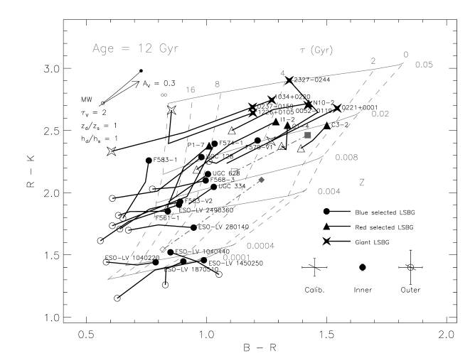
Figure 3: Galactic extinction and K-corrected $B-R$ and $R-K$ colours for our LSBG sample in three radial bins per galaxy: $0<r/h_{K}<0.5$ (solid symbols), $0.5<r/h_{K}<1.5$ and $1.5<r/h_{K}<2.5$ (open symbols). Circles denote the blue selected subsample of LSBGs, triangles the red selected subsample, and stars the giant LSBGs. Typical colour uncertainties in the inner and outer bins of the sample due to sky level errors are shown in the lower right hand corner. Calibration uncertainties are also shown. As $R$ band is used to form both colours, the effects of a typical 1$\sigma$ error in $R$ is also shown (diagonal line). Over-plotted are Bruzual & Charlot’s (in preparation) gissel98 stellar population models, and a foreground screen and Triplex model [Disney, Davies & Phillipps 1989, Evans 1994] dust reddening vector (see text for further details). Average Sa–Sc (grey squares) and Sd–Sm (grey diamonds) colours from de Jong [de Jong 1996a] at the centre (solid symbols) and at 2 disc scale lengths (open symbols) are also shown.

The main motivation for this programme of optical and near-IR imaging was to study the stellar populations of a diverse sample of LSBGs. In this section, we construct accurate colours as a function of radius for our sample and compare these colours with model stellar populations.

We first degrade all of the edited images of a given galaxy to the same angular resolution, and carry out surface photometry in three radial bins: $0<r/h_{K}<0.5$, $0.5<r/h_{K}<1.5$ and $1.5<r/h_{K}<2.5$, where $h_{K}$ is the $K$ band disc scale length. Galactic extinction corrections were taken from Schlegel et al. [Schlegel, Finkbeiner & Davis 1998, see Table 1]. K-corrections for the LSBG giants (as they are at non-negligible redshifts) were computed using non-evolving Sbc spectra from King & Ellis [King & Ellis 1985], and are typically 0.2 mag in $B$, negligible in $R$ and $-0.2$ mag in $K$. If required, $K^{\prime}$ magnitudes were converted $K$ magnitudes using the relation in Wainscoat & Cowie [Wainscoat & Cowie 1992], assuming a typical $H-K$ colour of $\sim$ 0.3 mag [de Jong 1996a]. The error in this correction is unlikely to exceed 0.05 mag.

We show Galactic extinction and K-corrected $B-R$ and $R-K$ colours for our sample of LSBGs in Fig. 3. Measurements in the three radial bins per galaxy are connected by solid lines, measurements of the central bin are denoted by a solid circle and measurements of the colours at two $K$ band disc scale lengths are denoted by open circles. Note that we only show colours with uncertainties smaller than 0.3 mag. Average zero point uncertainties and uncertainties in the inner and outer points due to sky level errors are also shown. Because $R$ band is used in both colour combinations, errors in $R$ band affect both colours. Accordingly, the average 1$\sigma$ $R$ band error is also shown (the short diagonal line). A $B-R$ against $R-K$ colour-colour plot was chosen to maximise the number of galaxies on the diagram. Other colour combinations (e.g. $B-V$ against $R-K$, etc.) limit the number of galaxies that can be plotted, but yield consistent positions on the stellar population grids. Note that P1-7 is placed on the plot assuming a $V-R$ colour of $0.40\pm 0.03$ (derived from the degenerate $B-V$ against $V-R$ colour-colour diagram using a typical galactic extinction corrected colour for P1-7 of $B-V\sim 0.57$).

Overplotted on the same diagram are stellar population models and model dust reddening vectors. We use the gissel98 implementation of the stellar population models of Bruzual & Charlot (in preparation). For Fig. 3 we adopt a Salpeter [Salpeter 1955] initial mass fuction (IMF) and an exponentially decreasing star formation rate characterised by an e-folding timescale $\tau$ and a single, fixed stellar metallicity $Z$ (where $Z=0.02$ is the adopted solar metallicity). For these models, the galaxy age (i.e. the time since star formation first started in the galaxy) is fixed at 12 Gyr. Note that the shape of the model grid is almost independent of galaxy age $\ga$ 5 Gyr. The solid grey lines represent the colours of stellar populations with a fixed metallicity and a variety of star formation timescales. The dashed grey lines represent the colours of stellar populations with different, fixed stellar metallicities and a given star formation timescale. There is some uncertainty in the shape and placement of the model grid: Charlot, Worthey and Bressan [Charlot, Worthey & Bressan 1996] discussed the sources of error in stellar population synthesis models, and concluded that the uncertainty in model calibration for older stellar populations is $\sim$ 0.1 mag in $B-R$ and $\sim$ 0.2 mag in $R-K$, which is roughly comparable to the calibration error bars in Fig. 3. The colour uncertainties are larger for some stellar populations than for others: e.g. the optical–near-IR colours for older, near-solar metallicity stellar populations are relatively secure, whilst the colours for younger, extreme metallicity stellar populations are much more uncertain. Other sources of systematic error include dust reddening and SFH uncertainties (as our assumption of a smoothly varying SFR is almost certainly unrealistic). For these reasons the positions of galaxies and colour trends between galaxies should be viewed relatively, e.g. that one class of galaxies is more metal-rich than another class of galaxies.

We also include vectors describing the effect of dust reddening using either a screen model (arrow) or the more realistic geometry of a Triplex dust model [Disney, Davies & Phillipps 1989, Evans 1994, curved line]. For the Triplex model a closed circle denotes the central reddening, and an open circle the reddening at 2.5 disc scale lengths. For both reddening vectors we use the Milky Way extinction law (and for the Triplex model, the albedo) from Gordon, Calzetti & Witt [Gordon et al. 1997]. Our Triplex model assumes equal scale length vertically and radially exponential dust and stellar distributions, and a central optical depth (for viewing a background object) in $V$ band of 2. These parameters are designed to be a reasonable upper limit to the effects of reddening in most reasonably bright spiral galaxies: Kuchinski et al. [Kuchinski et al. 1998] find from their study of 15 highly-inclined spiral galaxies that they are well-described by the above type of model, with central $V$ band optical depths of between 0.5 and 2. For the purposes of calculating the Triplex reddening vector, we use the optical depth due to absorption only for two reasons. Firstly, one might naïvely expect that for face-on galaxies at least as many photons will get scattered into the line of sight as out of it. Secondly, de Jong [de Jong 1996a] finds that an absorption-only Triplex model is a reasonably accurate description of the results of his realistic Monte-Carlo simulation (including the effects of both scattering and absorption) of a face-on Triplex geometry spiral galaxy.

4.1 Results

In the following interpretation of Fig. 3, we for the most part explicitly neglect the possible effects of dust reddening. There are a number of arguments that suggest that the effects of dust reddening, while present, are less important than stellar population differences both within and between galaxies. We consider these effects more carefully in section 4.2.2.

4.1.1 Colour gradients

The majority of the LSBGs in our sample with colours in at least two radial bins have significant optical–near-IR colour gradients. For the most part these colour gradients are consistent with the presence of a mean stellar age gradient, where the outer regions of galaxies are typically younger, on average, than the inner regions of galaxies. This is consistent with the findings of de Jong [de Jong 1996a] who concludes that age gradients are common in spiral galaxies of all types. Note that this is inconsistent with the conclusions of Bergvall et al. [Bergvall et al. 1999], who find little evidence for optical–near-IR colour gradients in their sample of blue LSBGs. However, their sample was explicitly selected to lack significant $B-R$ colour gradients, and so that we disagree with their conclusion is not surprising. The fact that Bergvall et al. managed to find galaxies without significant colour gradients is interesting in itself; while colour gradients are common amongst disc galaxies, they are by no means universally present. This is an important point, as by studying the systematic differences in physical properties between galaxies with and without colour gradients, it may be possible to identify the physical mechanism by which an age gradient is generated in disc galaxies.

There are galaxies which have colour gradients which appear inconsistent with the presence of an age gradient alone. The two early-type LSBGs C1-4 and C3-2 have small colour gradients which are more consistent with small metallicity gradients than with age gradients. In addition, a few of the bluer late-type LSBGs have colour gradients that are rather steeper than expected on the basis of age gradients alone, most notably F583-1 and P1-7, both of which appear to have colour gradients more consistent with a metallicity gradient. ESO 1040440 has an ‘inverse’ colour gradient, in that the central regions are bluer than the outer regions: this is probably due to a combination of very irregular morphology and the effects of foreground stellar contamination (which in this case makes the galaxy colours difficult to accurately estimate). There are also conspicuous ‘kinks’ in the colour profiles of F574-1 and 2327-0244, and a possible kink in the colour profile of UGC 128. In the case of F574-1, it is likely that the central colours of the galaxy are heavily affected by dust reddening. F574-1 is quite highly inclined ($67^{\circ}\pm 3^{\circ}$, assuming an intrinsic disc axial ratio $q_{0}$ of 0.15; Holmberg 1958) and shows morphological indications of substantial amounts of dust extinction in the INT 2.5-m $B$ and $V$ band images. This may also be the case for UGC 128, although the inclination is smaller in this case and there are no clear-cut morphological indications of substantial dust reddening. The LSBG giant 2327-0244 has a red nucleus in the near-IR, but a relatively blue nucleus in the optical. However, 2327-0244 is is a Seyfert 1 and has a central starburst [Terlevich et al. 1991], making our interpretation of the central colours in terms of exponentially decreasing SFR models invalid.

4.1.2 Colour differences between galaxies

In considering colour trends between LSBGs, we will first consider the star formation histories of different classes of LSBG, and then look at the star formation histories in a more global context.

Blue selected LSBGs

The majority of blue selected LSBGs, e.g. F561-1, UGC 334 and ESO-LV 2490360, are also blue in the near-IR. Their colours indicate that most blue selected LSBGs are younger than HSB late-types, with rather similar metallicities (compare the positions of the main body of blue selected LSBGs to the average Sd–Sm galaxy from de Jong’s sample). This relative youth, compared to the typically higher surface brightness sample of de Jong [de Jong 1996a] suggests that the age of a galaxy may be more closely related to its surface brightness than the metallicity is. We will come back to this point later in section 5.2.

Four out of the fifteen blue selected LSBGs fail to fit this trend: ESO-LV 1040220, ESO-LV 1040440, ESO-LV 1450250 and ESO-LV 1870510 all fall substantially ($\sim 0.3$ mag) bluewards of the main body of blue LSBGs in $R-K$ colour, indicating a lower average metallicity. While it should be noted that the South Pole subsample all have larger zero point uncertainties than the northern hemisphere sample, we feel that it is unlikely that the zero point could be underestimated so substantially in such a large number of cases. While the models are tremendously uncertain at such young ages and low metallicities, these optical–near-IR colours suggest metallicities $\la 1/10$ solar. This raises an interesting point: most low metallicity galaxies in the literature are relatively high density blue compact dwarf galaxies [Thuan, Izotov & Foltz 1999, Izotov et al. 1997, Hunter & Thronson 1995]. Thus, these galaxies and e.g. the blue LSBGs from Bergvall et al. [Bergvall et al. 1999] offer a rare opportunity to study galaxy evolution at both low metallicities and densities, perhaps giving us quite a different view of how star formation and galaxy evolution work at low metallicity.

Red selected LSBGs

In Bell et al. [Bell et al. 1999], we found that two red selected LSBGs (C1-4 and C3-2) were old and metal rich, indicating that they are more evolved than blue selected LSBGs. In this larger sample of five red selected LSBGs, we find that this is not always the case. The galaxies N10-2, C3-2, and C1-4 (with $B$ band central surface brightnesses $\sim$ 22.5 mag arcsec^-2) are comparitively old and metal rich, with central colours similar to old, near-solar metallicity stellar populations. However, I1-2 and P1-7 (with lower $B$ band central surface brightnesses $\sim$ 23.1 mag arcsec^-2) both have reasonably blue galactic extinction corrected optical–near-IR colours. I1-2 has a stellar population similar to de Blok et al.’s [de Blok, McGaugh & van der Hulst 1996] F579-V1, which is part of our blue selected subsample: these galaxies lie in the overlap between the two samples. P1-7 is relatively similar to other, brighter blue LSBGs such as UGC 128 and F574-1: it was included in the red selected subsample only by virtue of its relatively high foreground extinction $A_{B}=0.45$ mag.

Our limited data suggests that the red-selected LSBGs catalogued by O’Neil et al. [O’Neil et al. 1997a, O’Neil et al. 1997b] are a very heterogeneous group. Unlike the blue or giant LSBGs, the red-selected LSBGs seem to have relatively few common traits. The five red-selected LSBGs in this study seem to be a mix of two types of galaxy: i) early-type spirals or lenticulars which are genuinely red but have surface brightnesses $\mu_{B,0}\sim$ 22.5 mag arcsec^-2 at the upper range of the LSB class, and ii) objects with low surface brightnesses but colours that are not genuinely red. Objects in class ii) appear in the red-selected subsample due to large galactic foreground reddening and photometric errors.

Recently, O’Neil et al. [O’Neil et al. 1999] reported the detection of a small number of red, gas-rich LSBGs. These galaxies would clearly contradict our above interpretation of the red LSBGs, suggesting that at least some of the red LSBGs are a distinct (though potentially quite rare) class of galaxy. It is interesting to note that Gerritsen & de Blok [Gerritsen & de Blok 1999] predict that around 20 per cent of LSBGs should have $B-V\sim 1$ and relatively low surface brightnesses $\mu_{B,0}\ga 24.0$ mag arcsec^-2: these galaxies, which represent the fraction of the LSBG population that lack recent star formation, would appear to be both red and gas rich (blue LSBGs would be galaxies with exactly the same past SFH, but more recent star formation). However, note that O’Neil et al.’s result is subject to significant observational uncertainties: for example, the $B-V$ colour of P1-7 adopted by O’Neil et al. [O’Neil et al. 1999] is 0.9, whereas the foreground galactic extinction-corrected colour of P1-7 in this study is found to be 0.57$\pm$0.1. P1-7 is on the verge of being classified as a red, gas rich LSBG with a $B-V$ colour of 0.9, however it lies well within the envelope of blue, gas rich LSBGs with a galactic extinction corrected $B-V$ colour of 0.57. Proper observational characterisation of these red, gas rich LSBG candidates may prove quite crucial in testing LSBG formation and evolution models.

Giant LSBGs

LSBG giants have galactic extinction and K-corrected optical–near-IR colours which are similar to the redder LSBGs from O’Neil et al. [O’Neil et al. 1997a, O’Neil et al. 1997b], indicating central stellar populations that are reasonably old with roughly solar metallicity. However these central colours are not consistent with an old, single burst stellar population, although this conclusion is somewhat dependent on the choice of K-correction and model uncertainties (K-correction uncertainties are typically $\la$ 0.05 mag in each axis at 20000 km s^-1 for a change in galaxy type from Sbc to Sab, or Sbc to Scd). The outer regions of LSBG giants are much younger, on average, whilst still retaining near-solar metallicities. Comparing the $B-V$ and $R-K$ colours for the LSBG giants with some of the bluer HSB Sa–Sc galaxies in de Jong’s [de Jong 1996a] sample shows that both sets of galaxies have similar stellar populations. Thus, LSBG giants do not have unique SFHs (implying that there need be no difference in e.g. star formation mechanisms between the HSB Sa–Sc galaxies and the LSBG giants), however it is interesting that LSBG giants can have both a substantial young stellar population and a high metallicity, whilst possessing such low stellar surface densities (assuming reasonable stellar mass to light ratios).

Summary

Overall, there is a clear age and metallicity sequence, with red LSBGs and LSBG giants in the high stellar metallicity and older average age corner of the plot, progressing to the lower stellar metallicity and younger average age region of the plot for the blue LSBGs. This suggests that LSBGs, just like HSBGs, come in a variety of morphological types and SFHs; moreover, their morphologies and SFHs are linked.

4.2 Are the stellar population differences real?

4.2.1 Are IMF uncertainties important?

We have constructed Fig. 3 using a Salpeter [Salpeter 1955] IMF. However, the IMF is still reasonably uncertain, especially at the very low mass and high mass ends (see e.g. Elmegreen 1999, Scalo 1998). Variation of the low mass end of the IMF only significantly changes the (relatively ill-constrained) stellar mass to light ratio. Variation of the high mass end of the IMF, as illustrated by using e.g. the Scalo [Scalo 1986] or Miller & Scalo [Miller & Scalo 1979] IMF, only significantly changes the high metallicity, young stellar populations corner of the colour-colour plane: the colours in these regions are subject to considerable modelling uncertainties at any rate. We conclude that our results are robust to reasonable IMF uncertainties.

4.2.2 Dust reddening

We have interpreted Fig. 3 in terms of stellar population differences, however we have so far neglected the effects of dust reddening on the colours of our stellar populations. In Fig. 3 we show both a screen $A_{V}=0.3$ and absorption-only Triplex model $\tau_{V}=2$ dust reddening vector, both assuming Milky Way extinction and albedo curves. SMC extinction and albedo curves make little difference to the direction of the reddening vectors, but increases the length of the Triplex model reddening vector slightly because of the lower albedo at all wavelengths, compared to the Milky Way dust properties. The screen model vector is shown for illustrative purposes only, as the dust will be distributed roughly similarly to the starlight in realistic spiral galaxies, as assumed in the Triplex model.

The colour gradients in our sample of LSBGs are unlikely to be due to the effects of dust reddening for four reasons.

1. The optical depth that we choose for the Triplex model is on the high end of the plausible dust optical depths derived by Kuchinski et al. [Kuchinski et al. 1998].

2. The Triplex model assumes that all of the dust is distributed smoothly throughout the galaxy. In real galaxies typically 1/3 of the dust is gathered into optically thick clumps, which, when viewed face-on, simply tend to ‘drill holes’ in the light distribution but not produce any significant colour changes [de Jong 1996a, Kuchinski et al. 1998]. This dust would be more easily found in more edge-on galaxies, as in the edge-on orientation the probability of a clump along the line of sight is much larger than in a face-on disc. Therefore, Kuchinski et al.’s dust optical depths are likely to account for both the clumped and unclumped dust.

3. Most LSBGs have lower metallicity than their higher surface brightness counterparts. This implies that the dust to gas ratio should be lower in LSBGs than in HSBGs.

4. Only one galaxy in our sample, the starbursting Seyfert 1 2327-0244, has been detected by IRAS. This is in stark contrast to the diameter limited sample of de Jong & van der Kruit [de Jong & van der Kruit 1994], for which 78 per cent of the sample was detected by IRAS. This suggests that dust is much less important in LSBGs than in their higher surface brightness counterparts: indeed, many of the non-detections in de Jong & van der Kruit’s sample were LSBGs.

The above arguments suggest that the Triplex dust reddening vector in Fig. 3 is an upper limit to the real effects of dust reddening. Comparison of this upper limit on the dust reddening effects with the colour gradients in our sample suggests that most galaxies must have stellar population gradients to produce such pronounced colour gradients. This conclusion is supported by the direct modelling of Kuchinski et al. [Kuchinski et al. 1998], who use their own best-fit galaxy models to estimate the colour gradients in face-on spiral galaxies: they conclude that colour gradients as large as the ones we observe in LSBGs, or observed by de Jong [de Jong 1996a], are too large to arise solely from reddening by realistic amounts of dust. The same argument applies to relating different populations of LSBG: the amount of reddening required to make an intrinsically blue LSBG appear red is too large to be compatible with the observational evidence cited above.

5 Discussion

5.1 Quantifying the colour-colour plane

In section 4.1, we saw a pronounced age/metallicity sequence. LSBGs can have a diverse range of stellar populations: red selected LSBGs can be quite old and metal rich, whilst most blue selected LSBGs are much younger, and more metal poor. However, from Fig. 3 alone, it is difficult to see why the star formation histories of low surface brightness galaxies are as diverse as they are. For this reason, we have chosen to quantify the positions of galaxies on the colour-colour plane by assigning average ages and metallicities from the gissel98 stellar population models of Bruzual & Charlot (in preparation).

A finely interpolated grid of stellar population models was generated, covering a range of star formation timescales and metallicities. The metallicity ranges from $\langle Z\rangle=\log_{10}(Z/Z_{\sun})=-2.0$ (1/100 solar) to $\langle Z\rangle=0.4$ (2.5 times solar). In Fig. 3, we can see that some galaxies have optical–near-IR colours too blue to be described adequately by a constant star formation rate: for this reason, we must include exponentially increasing SFHs in our model grid. We include star formation timescales $\tau$ ranging from 0 (an average age of 12 Gyr) to $\infty$ (constant star formation with an average age of 6 Gyr) to $-1$ Gyr (an average age of 1 Gyr). We can see from the range of models included above that $\tau$ is an inappropriate parameter for describing the SFHs: we parameterise the SFH using the average age of the stellar population.

For each galaxy, the galactic extinction and K-corrected $B-R$ and $R-K$ colours between $0.5<r/h_{K}<1.5$ (when available; 0052-0119 and 0237-0159 have only central colours and are omitted from further consideration) are compared with the colours of the finely interpolated stellar populations grid. The quantity $\chi^{2}=\sum_{i=(B-V),(R-K)}(M_{i}-O_{i})^{2}/\sigma_{i}^{2}$ is minimised, where $M_{i}$ is the model colour, $O_{i}$ is the observed colour and $\sigma_{i}$ is the error in the observed colour. Error bars are obtained for the average ages and metallicities by fitting the colours plus or minus their 1$\sigma$ sky level and zero point errors added in quadrature.

This procedure has a number of limitations. Firstly, we neglect the effects of dust reddening. We considered the possible effects of dust earlier in section 4.2.2, and concluded that the effects of dust are fairly minimal for this sample. Our use of the colours between $0.5<r/h_{K}<1.5$ should act to further lessen the importance of dust reddening on our results. Secondly, because we use simple SFHs assuming a single metallicity, and because of stellar population model uncertainties, the ages and metallicities we determine are unlikely to be accurate in absolute terms. However, the idea of this simple analysis is to identify relative trends in SFH and metallicity, and their possible causes. The ages and metallicities we derive here will serve this purpose well: the optical–near-IR colours provide a robust way to order galaxies in terms of the relative importance of $\ga$ 5 Gyr old stars compared to younger $\la$ 2 Gyr old stars, which we parameterise using the average age of the stellar population. To better understand the relative uncertainties, we have also carried out the analysis using the stellar population models of Kodama & Arimoto [Kodama & Arimoto 1997]: the results obtained with their models are indistinguishable (in a relative sense) to the results presented in Figs. 4 and 5. An extended version of this analysis using all the available colour combinations for a much larger sample of galaxies will be presented in Bell & de Jong [Bell & de Jong 1999].

5.2 The correlations

Figure 4: Correlations between best-fit average ages, metallicities, $K$ central surface brightnesses, $K$ absolute magnitudes, $K$ disc scale lengths and gas fractions. Circles denote the blue selected subsample of LSBGs, triangles the red selected subsample, and stars the giant LSBGs. Note that the ages for the four ESO-LV galaxies near the low metallicity edge of the grid are highly uncertain: these points are denoted by naked error bars in all plots.

In order to understand what physical mechanisms might be driving the SFHs of LSBGs, we plot the best-fit average ages and metallicities against physical parameters, such as $K$ central surface brightnesses, $K$ absolute magnitudes, $K$ disc scale lengths and gas fractions. These correlations are presented in Fig. 4. Note that we do not attempt to provide a best fit or attach any kind of statistical significance to these relationships. We feel that this is over-interpreting this relatively limited dataset at this stage.

Galactic extinction and K-corrected $K$ absolute magnitudes are calculated using distances from Table 1. These absolute magnitudes are combined with the H i masses (multiplied by 1.33 to account for the helium mass fraction) from Table 1 to derive the gas fractions, using a $K$ band $M/L$ of 0.6 $M_{\sun}/L_{\sun}$ (c.f. Verheijen 1998; Chapter 6) and assuming a solar $K$ band absolute magnitude of 3.41 [Allen 1973]. Note that these gas fractions do not account for any molecular or hot gas component. The same distances are used to derive the $K$ band disc scale lengths in kpc. The $K$ band surface brightnesses have been corrected for galactic extinction, $K$ corrections, $(1+z)^{4}$ surface brightness dimming and inclination. Inclination corrections $C^{i}$ have been determined using an intrinsic edge-on disc axial ratio $q_{0}=0.15$ assuming that the disc is transparent; these corrections are given by:

$$C^{i}=-2.5\log_{10}(\frac{(1-e)^{2}-q_{0}^{2}}{1-q_{0}^{2}})^{1/2},$$ (1)

where $e$ is the adopted disc ellipticity from Table 8 [Holmberg 1958].

Before discussing Fig. 4, it is useful to note that the average ages of ESO-LV 1040220, 1040440, 1450250 and 1870510 are all potentially quite uncertain. This is due to their low metallicities: they have optical–near-IR colours suggesting metallicities $\la$ 1/100 solar metallicity (which falls off the model grid). At these metallicities, the model predictions (especially for young ages) are all rather uncertain. Therefore, we feel that their ages are less constrained (even in a relative sense) than their error bars otherwise suggest. These points are denoted by a naked set of error bars in Figs. 4 and 5. In the discussion that follows, we typically ignore the average ages for these four data points.

5.2.1 Limitations of our dataset

In Fig. 4, panel a, we show the relationship between $K$ band central surface brightness and $K$ band absolute magnitude in our dataset. In panels b and c, we show the relationship between gas fraction and $K$ band surface brightness and magnitude respectively. The main purpose of these panels is to simply show that in our sample of LSBGs, surface brightness, magnitude and gas fraction are quite strongly inter-related, and it is expected that correlations of any given quantity with surface brightness will be reflected by correlations of that same quantity with magnitude and gas fraction. Thus, on the basis of this dataset alone, it will be difficult to unambiguously differentiate between trends in the stellar populations of LSBGs driven by magnitude, trends driven by surface brightness, or trends driven by the gas fraction. Note that because of selection effects (primarily that we select only galaxies with low $B$ band surface brightness), panels a, b and c are unlikely to be representative of any universal correlation between surface brightness, magnitude and gas fraction.

5.2.2 Ages and metallicities

Fig. 4, panel d shows the correlation between the best-fit average age and metallicity. Ignoring the uncertain ages of the ultra-low metallicity LSBGs, there is a correlation, albeit a noisy one, between age and metallicity, in the sense that older galaxies tend to be more metal rich. This correlation quantifies the global trend between age and metallicity observed earlier in Fig. 3. This correlation is expected: galaxies appear old through a lack of recent star formation, implying a lack of gas (see also panel h, the age–gas fraction correlation). Most of our sample LSBGs are reasonably massive, meaning that their gas is unlikely to have been ejected by e.g. supernova driven winds. Therefore, their low gas fraction is likely to be due to consumption by star formation: this results in reasonably high stellar metallicities (see e.g. Pagel 1998). Note that some low surface brightness dwarf spheroidals may run counter to this argument, having low metallicities and reasonably old average ages (e.g. Mateo 1998): to explain this one would have to invoke removal of the gas from these low mass galaxies by e.g. supernova-driven winds [Dekel & Silk 1986] or, for cluster dwarf spheroidals, ram-pressure stripping [Abadi, Moore & Bower 1999].

5.2.3 Trends in LSBG age

In panels e, f, g and h, we show the trends in age with $K$ central surface brightness, $K$ absolute magnitude, $K$ disc scale length and gas fraction respectively. Age does not appear to correlate with disc scale length. Neglecting the uncertain ages of the four low metallicity ESO-LV galaxies, there appear to be trends in age with surface brightness, magnitude and gas fraction, in the sense that lower $K$ band surface brightness, lower $K$ luminosity and higher gas fraction LSBGs all have younger average ages. Furthermore, the scatter between age and surface brightness appears smaller than the scatter in the age–magnitude and age–gas fraction correlations. This suggests, tentatively, that the age–surface brightness correlation is the main correlation in this dataset, and the other correlations are the result of the magnitude–surface brightness and gas fraction–surface brightness correlations. We return to this issue later in section 5.3.

5.2.4 Trends in LSBG metallicity

In panels i, j, k and l of Fig. 4, we show the trends in LSBG metallicity with $K$ band surface brightness, magnitude, disc scale length and gas fraction. Note that the metallicities of the four low metallicity ESO-LV galaxies are reasonably well-constrained, therefore it is fair to include them in the discussion of these trends. Metallicity, unlike age, seems to be correlated with $K$ band disc scale length. This seems primarily because of the LSBG giants: they are bright and have large scale lengths, so their high metallicities will produce correlations between metallicity and magnitude and metallicity and scale length. It is likely that a metallicity–magnitude relation is more fundamental, however it is impossible to rule out scale length dependence in the metallicity on the basis of this dataset.

Metallicity, like age, seems to correlate well with $K$ band surface brightness, magnitude and gas fraction in the sense that LSBGs with lower metallicities have lower surface brightnesses, lower luminosities and higher gas fractions than LSBGs with higher metallicities. Both age and metallicity are also linked (panel d), so the similarity in trends with physical parameters between age and metallicity is not surprising. Again, as was the case for the age, it is more or less impossible to tell, on the basis of this dataset alone, which of the magnitude–metallicity or surface brightness–metallicity correlations are more fundamental.

5.3 SFH as a function of total mass and density

Figure 5: Correlations between best-fit average ages and metallicities and $K$ band surface brightnesses and magnitudes, modified by turning all of the available gas mass into stars with a $K$ band mass to light ratio of 0.6 $M_{\sun}/L_{\sun}$. Circles denote the blue selected subsample of LSBGs, triangles the red selected subsample, and stars the giant LSBGs: naked error bars denote the four low metallicity galaxies with potentially large age errors. Red selected or giant LSBGs at known distances for which there are no gas masses are shown as lower limits by error bars, with a solid triangle pointing towards the direction in which the galaxies move with increasing gas fraction: the vertex of the solid triangle denotes the modified surface brightness or magnitude assuming a gas fraction of 0.2. Panels c and f show the difference between the $B$ band absolute magnitude and the modified $K$ absolute magnitude and the difference between the $B$ band central surface brightness and modified $K$ band central surface brightness, respectively. Solid lines denote an average ‘colour’ $B-K_{\rm Modified}=3.9$, and the dashed line a scatter of 0.5 mag around this average.

In order to investigate how the baryonic mass and surface density affect the SFHs of LSBGs, we have modified the $K$ surface brightnesses and absolute magnitudes by turning the neutral gas fraction of the galaxy into stars using the correction to the magnitude $+2.5\log_{10}(1-f_{g})$. This correction assumes that the gas will turn into stars with the same $K$ band mass to light ratio as was assumed for the stellar population, which in this case is 0.6 $M_{\sun}/L_{\sun}$. This correction makes a number of assumptions.

1. The $K$ band mass-to-light ratio is expected to be relatively robust to the presence of young stellar populations, however our assumption of a constant $K$ band mass to light ratio is still a crude assumption. Note however that the relative trends in Fig. 5 are quite robust to changes in stellar mass-to-light ratio: as the stellar mass-to-light ratio increases, the modified magnitudes creep closer to their unmodified values asymptotically.

2. The presence of molecular gas is not accounted for in this correction. Assuming a typical galactic CO to H₂ conversion ratio, the non-detections of LSBGs by Schombert et al. [Schombert et al. 1990] and de Blok & van der Hulst [de Blok & van der Hulst 1998b] imply H₂ to H i ratios smaller than 0.25, and exceptionally as low as 0.04. This result is complicated by the expected metallicity dependence in the CO to H₂ conversion ratio [Mihos, Spaans & McGaugh 1999], however, molecular hydrogen is unlikely to dominate for all plausible values of the conversion factor.

3. The correction to the surface brightness implicitly assumes that the gas will turn into stars with the same spatial distribution as the present-day stellar component. This is a poor assumption as the gas distribution is usually much more extended than the stellar distribution; most LSBG gas distributions are centrally peaked however, and so the correction is unlikely to be completely wrong.

All of the above arguments suggest that the modified magnitudes and surface brightnesses are unlikely to give an accurate measure of the true masses and densities of LSBGs. These quantities do however better reflect the total mass and density of the galaxy than the $K$ band magnitudes and surface brightnesses alone, and so are useful as an indication of the kind of trends we might see if we could work out the baryonic masses and densities of LSBGs. The median correction is -0.9 mag, and 68 per cent of the corrections lie within 0.7 mag of this value.

The trends in age and metallicity with modified $K$ band central surface brightness and absolute magnitude are shown in Fig. 5. Three red and giant LSBGs with known redshifts but unknown (or unmeasurable) H i fluxes have been placed on Fig. 5 also: error bars denote their (unmodified) magnitudes or surface brightnesses, and solid triangles denote the direction that these galaxies move in with increasing gas fraction, with the vertex of the triangle indicating the offset that is produced by converting a gas fraction of 0.2 into stars. For reference, in panels c and f, we also show the relationship between $B$ band magnitude and surface brightness and the modified $K$ band magnitude and surface brightness. Surprisingly, we find that $B$ band magnitude and surface brightness are reasonable reflections of the modified magnitudes and surface brightnesses of LSBGs (remembering the uncertain assumptions that went into constructing the modified magnitudes and surface brightnesses). Both the $B$ band magnitudes and surface brightnesses have a mean offset from the modified $K$ band values consistent with a +3.9 mag offset, with an RMS of around 0.5 mag (solid and dotted lines in panels c and f). This relationship may be caused by the sensitivity of the optical mass to light ratios to recent star formation: $B$ band mass to light ratios decrease for younger populations in a such a way as to make the increase in brightness for younger populations offset almost exactly (to within a factor of 60 per cent or so, from the 0.5 mag scatter) by their larger gas fractions, making the $B$ band a reasonable total mass indicator in LSBGs (assuming that the $K$ band stellar mass to light ratio is fairly constant).

In panels a and b of Fig. 5, we see that the LSBG ages and metallicities correlate with their modified $K$ band magnitudes (baryonic masses). In stark contrast, in panels d and e, we see that the ages and metallicities correlate poorly with the modified $K$ band surface brightnesses (baryonic surface densities). This result is puzzling, especially in the light of the tight correlation between average age and surface brightness in panel e of Fig. 4. There are two possible interpretations of this huge scatter in the age–modified surface brightness plane.

Is it possible that there is little or no correlation between the SFH and surface density of a galaxy, as panels d and e suggest? In this case, we must explain the strong correlations between age and $K$ band surface brightness and metallicity and $K$ band surface brightness in panels e and i of Fig. 4. This may be possible to explain via selection effects: because we selected our galaxies to have a relatively narrow range of $B$ band surface brightness, and older, more metal rich galaxies are redder, we would naturally expect to see an artificial correlation between $K$ band surface brightness (which would be higher because of the redder colours) and age (which correlates with these red colours). Note, however, that this interpretation has real difficulty in explaining the tightness and dynamic range of the age–$K$ band surface brightness correlation.

Conversely, is it possible that there is a correlation between baryonic surface density and age, and that for some reason it is masked in this dataset? There is quite a narrow range (only $\sim$ 2 mag arcsec^-2) of modified surface brightness: the close correspondence between $B$ band and modified $K$ band surface brightnesses (panel f of Fig. 5) means that because we selected our galaxies to have a relatively narrow range of $B$ band surface brightness, we have implicitly selected for a narrow range in baryonic central surface density. Also, our modifications to the surface brightnesses were large for gas-rich galaxies with low $K$ band surface brightnesses and much smaller for gas-poor galaxies with higher $K$ band surface brightnesses, steepening the relationship between SFH and modified surface brightness considerably. Thus, we may simply lack an adequate surface density range to be able to distinguish a steep trend in age with surface density, especially in the presence of significant uncertainties in the ages and surface densities. Note that this is the interpretation that we prefer: the correlation between age and $K$ band surface brightness is quite tight, which is quite suggestive of some kind of correlation between density and SFH. Note that the age–mass relation would survive in this case relatively unscathed: the dynamic range for the age–mass relation is in excess of 5 magnitudes, which makes it quite robust to changes $\sim$ 1 mag in the relative positioning of the data points along the trend.

5.4 A unifying view

All the above correlations are consistent with the proposition that the age of a LSBG stellar population is primarily correlated with its surface density and that its metallicity is correlated with both surface density and mass, albeit with considerable scatter. Panels e, f, i and j of Fig. 4 all strongly support this scheme: in particular, LSBG giants have a range of $K$ band surface brightnesses (and ages; panel f) but have bright $K$ band absolute magnitudes (and high metallicities; panel j). The main obstacle for such a scenario is the lack of correlation between modified $K$ band surface brightnesses and age and metallicity, which may be due to our explicit selection of galaxies with only a relatively narrow range of $B$ band central surface brightness.

An important question to ask is if this scenario is physically plausible. A relationship between surface brightness/density and average age would be easy to understand: either a density dependent (e.g. Schmidt 1959) star formation law or a star formation timescale which is proportional to the local dynamical timescale would result in such a correlation (note that a magnitude–age correlation might suggest a global dynamical timescale dependence in the star formation law; e.g. Kennicutt 1998). Such a scenario would also very naturally account for the existence of age gradients in LSBGs: the outer regions of LSBGs are less dense, and would form stars less quickly than their inner regions, resulting in an age gradient.

Such a scheme is qualitatively consistent with those proposed by e.g. de Blok et al. [de Blok, McGaugh & van der Hulst 1996], Jimenez et al. [Jimenez et al. 1998] or Gerritsen & de Blok [Gerritsen & de Blok 1999]. In these schemes, it is primarily the low surface density that slows down the evolution of LSBGs (either explicitly through a density-dependent star formation law or implicitly, through an inability to build up a high gas metallicity). Metallicity’s mass dependence is likely to stem from the relative importance of feedback: the efficiency with which a galaxy ejects its metals in a supernova-driven wind is primarily driven by its mass [MacLow & Ferrera 1999].

While the above scenario is consistent with the data, it is unlikely to be unique: because of the correlation between surface brightness and magnitude, a purely mass-dependent age and metallicity may be plausible. Note, however that a mass-dependent age has some disadvantages: the ages of LSBG giants support a surface brightness dependent age, and age gradients would have to be explained using a different mechanism.

6 Conclusions

We have performed deep imaging of a sample of 26 LSBGs in the optical and near-IR in order to study their stellar populations. By comparing their optical–near-IR colours with the latest stellar population models, it is possible to constrain the young to old star ratio (parameterised by the average age of the galaxy) and the galaxy metallicity. We have found the following.

• Optical–near-IR colour gradients are common in LSBGs. Most colour gradients are consistent with a mean stellar age gradient, with the outer regions of galaxies appearing younger than the inner region of galaxies. We argue against the effects of dust reddening as the only cause of LSBG colour gradients. As common as colour gradients are, they are not present in all LSBGs [Bergvall et al. 1999]; this is important, because it may provide a chance to directly observe what drives the age gradient in LSBGs.

• We find that LSBGs have a wide range in morphologies and stellar populations, ranging from old, near solar metallicity populations for the very reddest LSBGs, to younger, high metallicity populations in the LSBG giants, to young and metal poor populations in the blue gas-rich LSBGs.

• By comparing the observed optical–near-IR colours between 0.5 and 1.5 disc scale lengths with stellar population models, we have determined best-fit average ages and metallicities that are robust in a relative sense, so that trends in age and metallicity will be quite secure.

• When the highly uncertain ages of the lowest metallicity galaxies are excluded, there are strong trends between both age and metallicity and $K$ band surface brightness, absolute magnitude and gas fraction. LSBGs with low $K$ band surface brightnesses, low $K$ luminosities and high gas fractions are all fairly unevolved, young, low metallicity systems. In contrast, LSBGs with higher $K$ band surface brightnesses, higher $K$ band luminosities and smaller gas fractions appear much more evolved, with older average ages and higher (near solar) metallicities.

• We have constructed crude estimates of the total mass and total densities of the atomic hydrogen, helium and stars in LSBGs by turning the gas into stars with a constant $K$ band mass to light ratio of 0.6 $M_{\sun}/L_{\sun}$. Surprisingly, we find that the $B$ band absolute magnitudes and surface brightnesses are reasonable predictors of the mass and density estimators, to within a factor of $\sim$ 60 per cent or so. We find that the ages and metallicities of LSBGs correlate well with our mass estimator, but correlate poorly with our surface density estimator. We argue that the poor correlation between our surface density estimator and SFH is the result of the narrow dynamic range in surface density probed by our sample, compounded by errors in SFH and density determination.

• Our results are consistent with a scenario in which the age of a LSBG is correlated primarily with its surface density, and the metallicity of a LSBG is correlated with both its surface density and mass (albeit with much scatter). This kind of correlation would be observed if the star formation law depended either explicitly on gas surface density or on the local dynamical timescale, and if the efficiency with which a galaxy retained its newly-synthesised metal content was a function of its mass.

References

- [Abadi, Moore & Bower 1999] Abadi M. G., Moore B., Bower R. G., 1999, MNRAS in press, astro-ph/9903436
- [Allen 1973] Allen C. W., 1973, “Astrophysical Quantities”, University of London, The Athlone Press
- [Barnaby et al. 1999] Barnaby D., Harper D. A., Loewenstein, R. F., Mrozek F., Thoma M., Lloyd J. P., Rauscher B. J., Hereld M., Severson S. A., 1999, PASP, submitted
- [Bell et al. 1999] Bell E. F., Bower R. G., de Jong R. S., Hereld M., Rauscher B. J., 1999, MNRAS, 302, L55
- [Bell & de Jong 1999] Bell E. F., de Jong R. S., 1999, MNRAS, submitted
- [Bergvall et al. 1999] Bergvall N., Rönnback J., Masegosa J., Östlin G., 1999, A&A, 341, 697
- [Block et al. 1994] Block D. L., Bertin G., Stockton A., Grosbøl P., Moorwood A. F. M., Peletier R. F., 1994, A&A, 288, 365
- [Block & Ivânio 1999] Block D. L., Ivânio P., 1999, A&A, 342, 627
- [Branchini et al. 1999] Branchini E. F., Teodoro L., Frenk C. S., Schmoldt I., Efstathiou G., White S. D. M., Saunders W., Rowan-Robinson M., Keeble O., Tadros H., Maddox S., Oliver S., Sutherland W., 1999, MNRAS, in press
- [Casali & Hawarden 1992] Casali M. M., Hawarden T. G., 1992, JCMT-UKIRT Newsletter, 3, 33
- [Charlot, Worthey & Bressan 1996] Charlot S., Worthey G., Bressan A., 1996, ApJ, 457, 625
- [de Blok & van der Hulst 1998a] de Blok W. J. G., van der Hulst J. M., 1998a, A&A, 335, 421
- [de Blok & van der Hulst 1998b] de Blok W. J. G., van der Hulst J. M., 1998b, A&A, 336, 49
- [de Blok, McGaugh & van der Hulst 1996] de Blok W. J. G., McGaugh S. S., van der Hulst J. M., 1996, MNRAS, 283, 18
- [de Blok, van der Hulst & Bothun 1995] de Blok W. J. G., van der Hulst J. M., Bothun G. D., 1995, MNRAS, 274, 235
- [de Jong 1996a] de Jong R. S., 1996a, A&A, 313, 377
- [de Jong 1996b] de Jong R. S., 1996b, A&AS, 118, 557
- [de Jong & van der Kruit 1994] de Jong R. S., van der Kruit P. C., 1994, A&AS, 106, 451
- [Dekel & Silk 1986] Dekel A., Silk J., 1986, ApJ, 303, 39
- [Disney, Davies & Phillipps 1989] Disney M. J., Davies J. I., Phillipps S., 1989, MNRAS, 239, 939
- [Elias et al. 1982] Elias J. H., Frogel J. A., Matthews K., Neugebauer G., 1982, AJ, 87, 1029
- [Elmegreen 1999] Elmegreen B. G., 1999, in “The Evolution of Galaxies on Cosmological Timescales”, eds. Beckman J. E. & Mahoney T. J., ASP Conference Series
- [Evans 1994] Evans R., 1994, PhD Thesis, University of Cardiff
- [Gerritsen & de Blok 1999] Gerritsen J. P. E., de Blok W. J. G., 1999, A&A, 342, 655
- [Gordon et al. 1997] Gordon K. D., Calzetti D., Witt A. N., 1997, ApJ, 487, 625
- [Holmberg 1958] Holmberg E., 1958, Medd. Lunds Astron. Obs. Ser., 2, No. 136
- [Huchtmeier & Richter 1989] Huchtmeier W. K., Richter O.-G., 1989, “A General Catalog of H i Observations of Galaxies”, New York, Springer-Verlag
- [Hunt et al. 1998] Hunt L. K., Mannucci F., Testi L., Migliorini S., Stanga R. M., Baffa C., Lisi F., Vanzi L., 1998, AJ, 115, 2594
- [Hunter & Thronson 1995] Hunter D. A., Thronson H. A., 1995, ApJ, 452, 238
- [Izotov et al. 1997] Izotov Y. I., Lipovetsky V. A., Chaffee F. H., Foltz C. B., Guzeva N. G., Kniazev A. Y., 1997, ApJ, 476, 698
- [Jimenez et al. 1998] Jimenez R., Padoan P., Matteucci F., Heavens A. F., 1998, MNRAS, 299, 123
- [Kennicutt 1998] Kennicutt R. C., Jr., 1998, ApJ, 498, 181
- [King & Ellis 1985] King C. R., Ellis R. S., 1985, ApJ, 288, 456
- [Kodama & Arimoto 1997] Kodama T. & Arimoto N., 1997, A&A, 320, 41 (KA97)
- [Kuchinski et al. 1998] Kuchinski L. E., Terndrup D. M., Gordon K. D., Witt A. N., 1998, AJ, 115, 1438
- [Landolt 1992] Landolt A. U., 1992, AJ, 104, 372
- [Lauberts & Valentijn 1989] Lauberts A., Valentijn E. A., 1989, “The surface photometry catalogue of the ESO-Uppsula galaxies.”
- [MacLow & Ferrera 1999] MacLow M.-M., Ferrera A., 1999, ApJ, 513, 142
- [Mateo 1998] Mateo M., 1998, ARA&A, 36, 435
- [McGaugh 1994] McGaugh S. S., 1994, ApJ, 426, 135
- [McGaugh & Bothun 1994] McGaugh S. S., Bothun G. D., 1994, AJ, 107, 530
- [McGaugh & de Blok 1997] McGaugh S. S., de Blok W. J. G., 1997, ApJ, 481, 689
- [McGaugh, Schombert & Bothun 1995] McGaugh S. S., Schombert J. M., Bothun G. D., 1995, AJ, 109, 2019
- [Mihos, Spaans & McGaugh 1999] Mihos J. C., Spaans M., McGaugh S. S., 1999, ApJ, 515, 89
- [Miller & Scalo 1979] Miller G. E., Scalo J. M., 1979, ApJS, 41, 513
- [Moshir et al. 1990] Moshir M., Kopan G., Conrow T., McCallon H., Hacking P., Gregorich D., Rohrbach G., Melnyk M., Rice W., Fullmer L., et al., 1990, ‘Infrared Astronomical Satellite Catalogs—The Faint Source Catalog’, Version 2.0.
- [Nguyen et al. 1996] Nguyen H. T., Rauscher B. J., Severson S. A., Hereld M., et al. , 1996, PASP, 108, 718
- [O’Neil et al. 1997a] O’Neil K., Bothun G. D., Cornell M. E., 1997a, AJ, 113, 1212
- [O’Neil et al. 1997b] O’Neil K., Bothun G. D., Schombert J. M., Cornell M. E., Impey C. D., 1997b, AJ, 114, 2448
- [O’Neil et al. 1999] O’Neil K., Bothun G. D., Schombert J. M., 1999, AJ, accepted, astro-ph/9909129
- [Padoan, Jimenez & Antonuccio-Delogu 1997] Padoan P., Jimenez R., Antonuccio-Delogu V., 1997, ApJ, 481, L27
- [Pagel 1998] Pagel B. E. J., 1998, “Nucleosynthesis and Chemical Evolution of Galaxies” (Cambridge University Press, Cambridge)
- [Persson et al. 1998] Persson S. E., Murphy D. C., Krzeminski W., Roth M., Rieke M. J., 1998, AJ, 116, 2475
- [Press et al. 1986] Press W. H., Flannery B. P., Teukolsky S. A., Vetterling W. T., 1986, Numerical Recipes—The Art of Scientific Computing (Cambridge University Press, Cambridge).
- [Quillen & Pickering 1997] Quillen A. C., Pickering T. E., 1997, astro-ph/9705115
- [Rauscher et al. 1998] Rauscher B. J., Lloyd J. P., et al., 1998, ApJ, 506, 116
- [Rauscher et al. 1999] Rauscher B. J., Lloyd J. P., et al., 1999, MNRAS, submitted
- [Richter, Tammann & Huchtmeier 1987] Richter O.-G., Tammann G. A., Huchtmeier W. K., 1987, A&A, 171, 33
- [Rönnback & Bergvall 1995] Rönnback J., Bergvall N., 1995, A&A, 302, 353
- [Salpeter 1955] Salpeter E. E., 1955, ApJ, 121, 61
- [Scalo 1986] Scalo J. M., 1986, Fundam. Cosmic Phys., 11, 1
- [Scalo 1998] Scalo J. M., 1998, in “The Stellar Initial Mass Function”, eds. Gilmore G. & Howell D., ASP Conference Series, 142, 201
- [Schlegel, Finkbeiner & Davis 1998] Schlegel D. J., Finkbeiner D. P., Davis M., 1998, ApJ, 500, 525
- [Schmidt 1959] Schmidt M., 1959, ApJ, 129, 243
- [Schneider et al. 1992] Schneider S. E., Thuan T. X., Magnum J. G., Miller J., 1992, ApJS, 81, 5
- [Schombert et al. 1990] Schombert J. M., Bothun G. D., Impey C. D., Mundy L. G., 1990, AJ, 100, 1523
- [Sprayberry et al. 1995] Sprayberry D., Impey C. D., Bothun G. D., Irwin M. J., 1995, AJ, 109, 558
- [Terlevich et al. 1991] Terlevich R., Melnick J., Masegosa J., Moles M., Copetti M. V. F., 1991, A&AS, 91, 285
- [Theureau et al. 1998] Theureau G., et al., 1998, A&AS, 130, 333
- [Thuan, Izotov & Foltz 1999] Thuan T. X., Izotov Y. I., Foltz C. B., 1999, astro-ph/9905345
- [van der Hulst et al. 1993] van der Hulst J. M., Skillman E. D., Smith T. R., Bothun G. D., McGaugh S. S., de Blok W. J. G., 1993, AJ, 106, 548
- [van Zee, Haynes & Salzer 1997] van Zee L., Haynes M. P., Salzer J. J., 1997, AJ, 114, 2479
- [Verheijen 1998] Verheijen M. A. W., 1998, PhD Thesis, University of Groningen
- [Wainscoat & Cowie 1992] Wainscoat R. J., Cowie L. L., 1992, AJ, 103, 332
- [Wegner, Haynes & Giovanelli 1993] Wegner G., Haynes M. P., Giovanelli R., 1993, AJ, 105, 1251