Orbital instability and relaxation in stellar systems

Abstract

We review recent progress in understanding the role of chaos in influencing the structure and evolution of galaxies. The orbits of stars in galaxies are generically chaotic: the chaotic behavior arises in part from the intrinsically grainy nature of a potential that is composed of point masses. Even if the potential is assumed to be smooth, however, much of the phase space of non-axisymmetric galaxies is chaotic due to the presence of central density cusps or black holes. The chaotic nature of orbits implies that perturbations will grow exponentially and this in turn is expected to result in a diffusion in phase space. We show that the degree of orbital evolution is not well predicted by the growth rate of infinitesimal perturbations, i.e. by the Liapunov exponent. A more useful criterion is whether perturbations continue to grow exponentially until their scale is of order the size of the system. We illustrate these ideas in a potential consisting of $N$ fixed point masses. Liapunov exponents are large for all values of $N$, but orbits become increasingly regular in their behavior as $N$ increases; the reason is that the exponential divergence saturates at smaller and smaller distances as $N$ is increased. The objects which lend phase space its structure and impede diffusion are the invariant tori. In the triaxial potentials we discuss, a large fraction of the tori correspond to resonant (thin) orbits and their associated families of regular orbits. These tori are destroyed by perturbations to the potential. When only a few stable resonances remain, we find that the phase space distribution of an ensemble of chaotic orbits evolves rapidly toward a nearly stationary state. This mixing process is shown to occur on timescales of a few crossing times in triaxial potentials containing massive central singularities, consistent with the rapid evolution observed in $N$-body simulations of galaxies with central black holes.

1 Introduction

The role of microscopic chaos in producing macroscopic relaxation of dynamical systems has received considerable attention in the field of statistical mechanics ([Lebowitz 1993], [Gaspard 1998]). However, the role of chaos in the relaxation of stellar systems is relatively less well understood. The last five years have witnessed the development of a number of new techniques for probing the complexities of phase space in realistic galactic potentials. This work has led to a greater understanding of the importance of stochastic orbits and their role in driving dynamical evolution.

The gravitational forces on a star in a galaxy can be broken up into two components: a rapidly varying component that arises from the discrete distribution of stars, and a smoothly varying component that arises from the overall mass distribution. The importance of the discrete component of the force relative to the smooth component is usually assumed proportional to $\sim 10\ln{N}/N$, the ratio of dynamical to two-body relaxation times ([Chandrasekhar 1943]). The implication is that, for galaxies ($N\sim 10^{11}$), the time scale on which the discrete component of the force is important is much longer than the age of the Universe. At the same time, it has been shown ([Miller 1964], [Gurzadyan & Savvidy 1986]) that trajectories in the $N$-body problem are generically chaotic, with rates of exponential divergence that appear to remain large even for large $N$. Thus, according to at least one definition of chaos, the orbits of stars in galaxies should never tend toward the regular motion expected in smooth potentials.

The exponential divergence of trajectories gives rise to a diffusion. The approach of a non-stationary distribution of phase points to a stationary one via chaotic diffusion is referred to as “chaotic mixing” or just “mixing” ([Kandrup & Mahon 1994]). In the context of non-equilibrium statistical mechanics, mixing to an invariant distribution is regarded as a legitimate relaxation process ([Lebowitz 1993], [Gaspard 1998]). However, in the context of gravitational systems, the issue of whether or not there is a connection between the time scale for exponential divergence of adjacent trajectories and the time scale for macroscopic relaxation has been a matter of much debate ([Gurzadyan & Savvidy 1986], [Kandrup 1990], [Kandrup & Smith 1991], [Heggie 1991], [Goodman et al. 1993]).

The question of how and under what conditions chaos will result in evolution of a stellar system is the subject of this article. In §2 we present two idealized models: a set of $N$ fixed mass points, representing stars in a galaxy; and a smooth potential with a single central point mass, representing a galaxy with a nuclear black hole. Motion in both potentials is generically chaotic, with similar values of the Liapunov exponent. We show that the Liapunov exponent – which measures only the infinitesimal growth of perturbations – is not always useful for predicting the degree of macroscopic evolution. A more useful criterion is whether perturbations continue to grow exponentially until their size is of order the size of the system. The kinds of structures that can impede diffusion of stochastic orbits are discussed in §3. In §4 we simulate the approach to an invariant distribution of stars in galactic potentials; we find that evolution to a stationary state can take place in little more than a crossing time if the phase space is globally chaotic. Such evolution is consistent with the rapid, self-consistent evolution observed in numerical simulations of galaxies containing nuclear black holes.

2 The Liapunov exponent and other measures of chaos

Exponential divergence of nearby trajectories is a common property of dynamical systems. This divergence is most commonly expressed in terms of the Liapunov exponent, which measures the mean $e$-folding rate of an infinitesimal perturbation averaged over an infinite time interval. Because the perturbation is assumed to remain small, Liapunov exponents measure only the rate of divergence in the immediate vicinity of the unperturbed orbit; they do not necessarily contain any information about the non-linear, or macroscopic, evolution. One might nevertheless expect the magnitude of the Liapunov exponent to predict, in some approximate sense, the degree to which chaos will induce finite changes in the structure of an orbit after a fixed time. This turns out not always to be the case, as we now illustrate.

Figures 1 and 2 summarize the results of test-particle integrations in two time-independent potentials. Model 1 (Fig. 1) consists of $N$ point masses $m$ distributed randomly and uniformly within a triaxial ellipsoid; the total mass $M=Nm$ remains fixed ($M=1$) as $N$ is varied, as do the axis lengths ($a=1,b=0.75,c=0.5$) of the ellipsoid. Model 2 (Fig. 2) is the smooth representation of Model 1, i.e. a homogeneous ellipsoid, to which has been added a single central point of mass $M_{h}$. The parameter $N$ of Model 1 may be interpreted as the number of stars that make up a galaxy of fixed mass, and the parameter $M_{h}$ of Model 2 as the mass of a central black hole, expressed in units of the total galaxy mass. The quantities $1/N$ and $M_{h}$ play the role of perturbation parameters; as they are increased, the potential departs more and more from that of the integrable, 3D harmonic oscillator, and one expects to see corresponding changes in the behavior of orbits.

Figure 1: Evolution of orbits in a potential consisting of $N$ fixed point masses, $m=1/N$, distributed randomly and uniformly in an ellipsoidal volume. For each $N$, 32 random realizations of the particle positions were generated and a single orbit was integrated in each of the corresponding potentials. The upper left panel shows mean values of the Liapunov exponent $\sigma$ for each ensemble, and the RMS variation in the “action” $J_{x}$ over $\sim 20$ orbital periods (see text). $\sigma$ remains large while $\delta J_{x}$ falls off with $N$; thus the behavior of a typical orbit becomes more and more regular as $N$ increases. This is verified in the lower left panel which shows typical orbits for four values of $N$. The lower right panel displays the finite separation between initially adjacent trajectories. While the divergence takes place at the rate predicted by the Liapunov exponents at early times, for large $N$ the separation saturates at a value much smaller than the size of the system.

The evolution of orbits in Model 1 is illustrated in Fig. 1, as a function of the number of particles making up the potential. For each $N$, a set of 32 random realizations of the particle positions were generated; a single orbit was then integrated in each of the 32 corresponding potentials. The evolution of the orbits were measured in several ways. The mean Liapunov exponent $\sigma$ (averaged over the 32 ensembles) was found to increase with $N$ until $N\approx 100$ then level off, at a value $\sigma T_{cr}\sim 5$, with $T_{cr}$ defined as one-half of the long-axis orbital period in the smooth potential. Thus these trajectories are locally unstable on a remarkably short time scale, just a fraction of a crossing time, and this characteristic time shows no tendency to decrease with increasing $N$ for $N$ as large as $\sim 10^{5}$. This result is similar to the well-known exponential instability of the full $N$-body problem ([Miller 1964], [Gurzadyan & Savvidy 1986], [Kandrup 1990], [Kandrup & Smith 1991], [Heggie 1991], [Goodman et al. 1993]).

As a second measure of the orbital evolution, the RMS variations in the $x$, $y$ and $z$ “actions” of the orbits were computed over $\sim 20$ periods; these “actions” were defined in terms of the frequencies of motion in the smooth potential, e.g. $J_{x}=E_{x}/\omega_{x}=(v_{x}^{2}+\omega_{x}x^{2})/(2\omega_{x})$, and would be precisely conserved in the limit of zero perturbation. Figure 1 shows that there is a smooth decrease in the amplitude of $\delta J_{x}$ as $N$ is increased – in other words, the orbits approach more and more closely, in their macroscopic behavior, to that of the integrable orbits even though they remain locally unstable to a degree (as measured by $\sigma$) that is nearly independent of $N$. Plots of the trajectories (Fig. 1) confirm that the orbits for large $N$ are similar to the Lissajous figures expected in the 3D harmonic oscillator.

This apparent paradox – large $\sigma$, but nearly regular motion – is reconciled in the lower right panel of Fig. 1, which shows the variation with time of the finite separation between two initially nearby trajectories, for four values of $N$. The divergence is initially exponential in all cases, with a characteristic time $\sim 0.2T_{cr}$, consistent with the measured values of $\sigma$. However the exponential divergence eventually saturates, after which the separation slows. This saturation has no effect on the Liapunov exponents which are calculated assuming that the separation remains infinitesimally small. Furthermore, the saturation occurs sooner for larger $N$. When $N\mathrel{\mathchoice{\lower 3.6pt\vbox{\halign{$\mathsurround=0pt\displaystyle\hfil#\hfil$\cr<\crcr\sim\crcr}}}{\lower 3.6pt\vbox{\halign{$\mathsurround=0pt\textstyle\hfil#\hfil$\cr<\crcr\sim\crcr}}}{\lower 3.6pt\vbox{\halign{$\mathsurround=0pt\scriptstyle\hfil#\hfil$\cr<\crcr\sim\crcr}}}{\lower 3.6pt\vbox{\halign{$\mathsurround=0pt\scriptscriptstyle\hfil#\hfil$\cr<\crcr\sim\crcr}}}}10^{3}$, the exponential divergence continues until the separation is of order the size of the system, while for $N\approx 10^{5}$, saturation occurs at a separation of only $\sim 10^{-2}$, much smaller than the system size.

How can the separation between two, locally unstable orbits saturate at a small amplitude, given that neither orbit “knows” about the other orbit? The answer must be that both orbits are confined to the same, restricted region of phase space; saturation occurs when the separation between them is of order the width of this region. Further systematic increase in their separation would require that one of the trajectories “break out” into another such region, and such events (for large $N$) apparently occur at a much lower rate than the divergence described by the Liapunov exponent. The fact that the exponential divergence saturates sooner for larger $N$ suggests that the width of the confining regions decreases with increasing $N$ – although our experiments do not allow us to estimate the precise $N$-dependence. The apparently unconfined evolution for $N\mathrel{\mathchoice{\lower 3.6pt\vbox{\halign{$\mathsurround=0pt\displaystyle\hfil#\hfil$\cr<\crcr\sim\crcr}}}{\lower 3.6pt\vbox{\halign{$\mathsurround=0pt\textstyle\hfil#\hfil$\cr<\crcr\sim\crcr}}}{\lower 3.6pt\vbox{\halign{$\mathsurround=0pt\scriptstyle\hfil#\hfil$\cr<\crcr\sim\crcr}}}{\lower 3.6pt\vbox{\halign{$\mathsurround=0pt\scriptscriptstyle\hfil#\hfil$\cr<\crcr\sim\crcr}}}}10^{3}$ suggests that phase space for such small $N$ is “globally chaotic”, with essentially no confining barriers.

Figure 1 suggests the way in which the equations of motion in an $N$-body potential tend toward those of the corresponding smooth potential as $N$ increases. Although some measures of chaos – e.g. the Liapunov exponents – remain large even for large $N$, others – e.g. the change in the actions – tend to zero.

Figure 2: Like Fig. 1, for orbits in the potential of a uniform triaxial ellipsoid of unit mass with an added central point of mass $M_{h}$. A single orbit was integrated for each value of $M_{h}$ and its properties recorded. Both the Liapunov exponent $\sigma$ and the variation in the “action” $\delta J_{x}$ fall off with decreasing $M_{h}$. However, as in Fig. 1, the trajectories can mimic regular orbits for times much longer than $\sigma^{-1}$ when $M_{h}$ is small. The lower right panel again shows why: for small $M_{h}$, the evolution of the finite separation between initially adjacent trajectories is not well predicted by the Liapunov exponent.

These results present an interesting contrast with those from Model 2 (Fig. 2). Here a single orbit was integrated for each value of $M_{h}$, the mass of the central “black hole,” in the otherwise smooth, harmonic-oscillator potential. Both $\sigma$ and $\delta J_{x}$ were now found to vary systematically with perturbation parameter $M_{h}$; thus the orbits tend toward regularity with decreasing $M_{h}$ as measured both by their infinitesimal and finite-amplitude behaviors. But the lower right-hand panel of Fig. 2 reveals essential similarity with the behavior of the orbits in Model 1. For large black hole masses, $M_{h}\mathrel{\mathchoice{\lower 3.6pt\vbox{\halign{$\mathsurround=0pt\displaystyle\hfil#\hfil$\cr>\crcr\sim\crcr}}}{\lower 3.6pt\vbox{\halign{$\mathsurround=0pt\textstyle\hfil#\hfil$\cr>\crcr\sim\crcr}}}{\lower 3.6pt\vbox{\halign{$\mathsurround=0pt\scriptstyle\hfil#\hfil$\cr>\crcr\sim\crcr}}}{\lower 3.6pt\vbox{\halign{$\mathsurround=0pt\scriptscriptstyle\hfil#\hfil$\cr>\crcr\sim\crcr}}}}0.02$, divergence continues at roughly the Liapunov rate until the orbits are separated by of order the size of the system; while for $M_{h}\mathrel{\mathchoice{\lower 3.6pt\vbox{\halign{$\mathsurround=0pt\displaystyle\hfil#\hfil$\cr<\crcr\sim\crcr}}}{\lower 3.6pt\vbox{\halign{$\mathsurround=0pt\textstyle\hfil#\hfil$\cr<\crcr\sim\crcr}}}{\lower 3.6pt\vbox{\halign{$\mathsurround=0pt\scriptstyle\hfil#\hfil$\cr<\crcr\sim\crcr}}}{\lower 3.6pt\vbox{\halign{$\mathsurround=0pt\scriptscriptstyle\hfil#\hfil$\cr<\crcr\sim\crcr}}}}0.01$, the evolution of the separation is more complex, with periods of stagnation followed by sudden jumps (when the trajectory passes sufficiently close to the central point). Once again, we postulate that the phase space of potentials with $M_{h}\mathrel{\mathchoice{\lower 3.6pt\vbox{\halign{$\mathsurround=0pt\displaystyle\hfil#\hfil$\cr>\crcr\sim\crcr}}}{\lower 3.6pt\vbox{\halign{$\mathsurround=0pt\textstyle\hfil#\hfil$\cr>\crcr\sim\crcr}}}{\lower 3.6pt\vbox{\halign{$\mathsurround=0pt\scriptstyle\hfil#\hfil$\cr>\crcr\sim\crcr}}}{\lower 3.6pt\vbox{\halign{$\mathsurround=0pt\scriptscriptstyle\hfil#\hfil$\cr>\crcr\sim\crcr}}}}0.01$ is globally stochastic, with few impediments to the motion – a conjecture that was actually verified ([Valluri & Merritt 1998]) in a different class of triaxial potentials (see §3). For smaller $M_{h}$, the orbital evolution consists of a sequence of nearly-random transitions from one, approximately regular orbit to another ([Gerhard & Binney 1985]); these transitions become rarer as $M_{h}$ is reduced.

These experiments suggest that Liapunov exponents are not good predictors of the macroscopic behavior of orbits. Even trajectories with large $\sigma$ can exhibit nearly regular behavior over time scales much longer than $\sigma^{-1}$. In deciding whether stochasticity is likely to be important for the behavior of orbits, the crucial question is not the value of $\sigma$, but whether the exponential divergence continues until separations of order the size of the system are reached. If the separation saturates at some value much smaller than the system size, orbital stochasticity may not be of much consequence even if $\sigma$ is large.

The sorts of structures that can impede the diffusion of stochastic orbits are described in more detail in the next section. Here we note that even some very simple dynamical models can exhibit the basic properties that we have described. For instance, the motion of particles in a “Lorentz gas,” a fixed 2D array of cylindrical scatters, is generically stochastic, with Liapunov times of order the time between collisions. However in the close-packed limit, trajectories are blocked by the finite size of the scatterers, causing them to remain confined to narrow regions for long periods of time ([Gaspard 1998]). Thus the exponential instability has little consequence for the macroscopic character of the motion.

3 Phase space structure of triaxial galaxies

In an integrable potential with $N$ degrees of freedom (DOF), all the trajectories have exactly $N$ isolating integrals and are confined to $N$-dimensional tori in phase space. Such a torus is defined by the $N$ actions ${\bf J}$ that fix its cross-sectional areas. Motion around this torus occurs at a rate determined by a constant frequency vector ($\omega_{1},\omega_{2},...,\omega_{N}$). Realistic potentials with more than 1 DOF are rarely integrable and the motion is more complex. While the KAM theorem guarantees that most of the original tori will persist when an integrable system is slightly perturbed, even under small perturbations a large part of the phase space will be influenced by resonances. A resonant torus is one which satisfies (one or more) resonant conditions of the form $n.\omega$$=0$ between the $N$ fundamental frequencies. Such tori are dense in the phase space of the integrable potential but typically only the lowest order resonances have a significant influence on the motion in the perturbed potential ([Lichtenberg & Lieberman 1992]). In the vicinity of a stable resonant torus, motion is still regular, but the orbits have shapes determined by the order of the resonance – often very different from the shapes of orbits in the integrable potential. In the vicinity of unstable resonant tori, trajectories are usually chaotic.

In a system with 2 DOF, the resonant tori are closed periodic orbits defined by a single frequency $\omega_{0}=n_{2}\omega_{1}=n_{1}\omega_{2}$. In 3 DOF the resonant tori obey a condition on the three fundamental frequencies of the form $n_{1}\omega_{1}+n_{2}\omega_{2}+n_{3}\omega_{3}=0.$ Such a relation does not imply that the orbit is closed, as in 2 DOF, but rather that it is thin, densely filling a sheet in configuration space ([Merritt & Valluri 1999]). The resonance condition can be used to reduce the number of independent frequencies by one; the two remaining frequencies then describe the rate of rotation around the 2D reduced torus ([Carpintero & Aguilar 1998], [Merritt & Valluri 1999]). In 3 DOF systems as in 2 DOF systems, resonant tori are the regions where perturbation expansions fail, and where the the global structure of phase space is expected to be changed. Thus the thin orbits are expected to play a similar role in 3 dimensions to the role played by periodic orbits in 2 dimensions.

Families of thin orbits may exist even in an integrable potential if it contains “primary resonances” that divide up the phase space ([Lichtenberg & Lieberman 1992]). This is the case in the well-known “perfect ellipsoid” ([Kuzmin 1973], [de Zeeuw 1985]): the $1:1$ closed orbits in the principal planes generate families of thin tube orbits. In non-integrable potentials, one expects to find thin orbits and their associated families throughout phase space.

One of the most useful tools to be employed recently in the study of galactic potentials is the frequency analysis technique (NAFF) developed by Laskar ([Laskar 1990], [Laskar et al. 1992], [Laskar 1998]). Laskar’s technique exploits the fact that regular orbits are quasiperiodic: Cartesian coordinates like $x(t)$ and $v_{x}(t)$ can be expressed as Fourier series in terms of the three fundamental frequencies on the torus. While this basic principle has been used to study orbits in the past ([Binney & Spergel 1984]), Laskar showed that the accuracy with which the individual frequency components can be extracted is greatly improved by employing a Fourier filtering function and by orthogonalizing successive frequency components. Once the entire frequency spectrum is obtained, the three fundamental frequencies $(\omega_{1},\omega_{2},\omega_{3})$, which appear as linear combinations in each line, may be identified using an integer programming algorithm ([Valluri & Merritt 1998]). All the lines in the spectrum are then immediately expressible in terms of the fundamental frequencies, giving a map between the action-angle and Cartesian coordinates ([Valluri & Merritt 1999b]).

Strictly speaking, only regular orbits are restricted to tori and amenable to Laskar’s technique. Nonetheless, as discussed above, stochastic trajectories may mimic regular orbits for long periods of time. On short time scales, such an orbit has a frequency spectrum which mimics a quasi-periodic series. As the orbit diffuses through phase space, its frequency spectrum will change. Laskar ([Laskar 1993]) showed that over a fixed interval of time ($\Delta T)$ the change in the frequency of the leading term in the spectrum, $\Delta\omega=|\omega(T)-\omega(T+\Delta T)|$, is a good measure of the rate of diffusion of a chaotic orbit in phase space. Note that Laskar’s $\Delta\omega$, unlike the Liapunov exponent, measures a finite excursion in phase space. In this sense it is similar to the $\delta J$ parameter defined above.

Since Laskar’s technique maps the structure of phase space in the frequency domain, it is ideally suited to identifying the resonant tori. In 2 DOF galactic potentials, Papaphillipou & Laskar ([1996]) showed that in a map of $\omega_{1}/\omega_{2}$ versus a third parameter, resonant families appear as regions where $\omega_{1}/\omega_{2}=$ const over some set of orbits. In 3DOF systems, a “frequency map” may be obtained by plotting the ratios $\omega_{1}/\omega_{3}$ versus $\omega_{2}/\omega_{3}$ ([Papaphillipou & Laskar 1998]). Here the resonant families show up as lines of constant slope. Thus by constructing a frequency map of an ensemble of orbits chosen from a regular grid of starting values, it is possible to locate the resonances which significantly affect the structure of phase space.

Another useful device is the “diffusion map”: a plot of the chaotic diffusion rates $\Delta\omega$ ([Laskar 1993]). We calculated diffusion maps for a family of galaxy models which are triaxial generalizations of the spherical models described by Dehnen ([1993]) and others. These models provide a good fit to the inner part of the light distributions of real galaxies and have a mass density given by

$$\rho(m)={(3-\gamma)M\over 4\pi abc}m^{-\gamma}(1+m)^{-(4-\gamma)},\ \ \ \ 0\leqslant\gamma<3$$ (1)

with

$$m^{2}={x^{2}\over a^{2}}+{y^{2}\over b^{2}}+{z^{2}\over c^{2}},\ \ \ \ a\geqslant b\geqslant c\geqslant 0,$$ (2)

and $M$ the total mass. The mass is stratified on ellipsoids with axis ratios $a:b:c$; the $x$ and $z$ axes are the long and short axes respectively. The parameter $\gamma$ determines the slope of the central, power-law density cusp.

Figure 3: Resonances in triaxial potentials. The mass model in (a) has a weak ($\gamma=0.5$) cusp and no black hole; in (b) the black hole contains $0.3$% of the total mass. Both equipotential surfaces lie close to the half-mass radius. The grey scale measures the degree of stochasticity of orbits started with zero velocity on the equipotential surface. Stable resonance zones – the white bands in (a) and (b) – are labeled by the order $(n_{1},n_{2},n_{3})$ of the resonance. Panels (c) and (d) show the pericenter distance $\Delta$ of a set of $10^{3}$ orbits with starting points lying along the heavy solid lines in (a) and (b).

Figures 3a,b show the diffusion maps at one energy in a triaxial Dehnen potential with $\gamma=0.5$, with and without a central black hole. Orbits were integrated starting at rest on the equipotential surface just inside the half-mass radius of the model. The diffusion rate ($\Delta\omega$) was plotted in grey scale on the equipotential surface. Rapidly diffusing (chaotic) orbits are coded in black while regular orbits ($|\Delta\omega|\approx 0$) are shaded white. The intensity of the grey scale is proportional to the logarithm of the stochastic diffusion rate as measured by $|\Delta\omega|$. The resonant tori and their associated families appear as narrow white bands and are marked in the figure by their defining integers $n_{1},n_{2},n_{3}$. The white bands are flanked by thin dark ones which are the stochastic layers marking the transitions between resonant families. Some of these resonances – the (2, 0 -1) banana; the (4, -3,0) pretzel; and the (3,0,-2) fish – are 2D resonances that correspond to periodic orbits in one of the principal planes. Miralda-Escudé & Schwarzschild ([1989]) call such orbits “boxlets”. However most of the resonant families cannot be associated with a periodic orbit.

A striking feature of Fig. 3a is the large number of narrow but distinct resonance zones. The reason for the narrowness is suggested by Fig. 3c which shows the distance of closest approach to the potential center of a set of orbits whose initial conditions lie along the heavy curve in Fig. 3a. As one passes through a stable resonance, the orbital pericenter reaches a maximum on the resonance where the orbit has zero thickness. The width of the resonance band is set by how thick an orbit can become before it is rendered stochastic – this happens when the distance of closest approach to the destabilizing center is sufficiently small. In potentials with a steep central force, this destabilization is attributable to gravitational deflections which occur when the trajectory passes near the center. In the case of the $\gamma=0.5$ model of Fig. 3a, the force is analytic all the way to $r=0$. Here, the orbits become chaotic because they come arbitrarily close to an unstable “separatrix” layer which marks the transition between one resonant family and the next. Once a family is wide enough to pass through the center it can no longer maintain the same fundamental “shape” properties (i.e. it can no longer be characterized by the same $(n_{1},n_{2},n_{3})$ values). This results in a transition to a new family of orbits. This transition from one resonant family to another is reminiscent of the transition from tube to box orbits, which occurs even in integrable potentials ([de Zeeuw 1985]). The lowest-order resonant orbits, have simple shapes and the largest central “holes” allowing a large family of associated regular orbits. Higher-order resonances have more complex shapes and pass nearer the center; their associated families, and their resonance bands in Fig. 3a, are correspondingly smaller.

Figure 3b shows a diffusion map for a $\gamma=0.5$ model with a central black hole of mass $M_{h}=0.003M$. In this figure the stochastic regions between the resonant families are significantly wider. Figure 3d shows that the black hole destabilizes orbits well before they become thick enough to pass through the center – somewhat different from the standard picture ([Gerhard & Binney 1985]) in which box orbits are destabilized by passing arbitrarily close to a central black hole.

As the mass of a central point is increased, more and more of the resonant tori are rendered unstable, and the width of the stochastic layers and their degree of overlap are increased. Figure rotation has a similar effect ([Valluri 1999]). One finds ([Valluri & Merritt 1998], [Merritt & Valluri 1999]) that the phase space of box-like orbits (orbits with stationary points) becomes “globally chaotic” when such perturbations are sufficiently large – there are essentially no stable invariant tori left. For instance, in non-rotating triaxial potentials, global chaos ensues when the central point contains $\sim 10^{-2}$ of the galaxy mass within the equipotential surface. In the globally chaotic regime, there are few barriers to the motion and one expects orbital evolution to be very rapid and extensive. Figure 2 confirms this prediction in the case of motion in a homogeneous ellipsoid.

4 Chaotic mixing and dynamical evolution

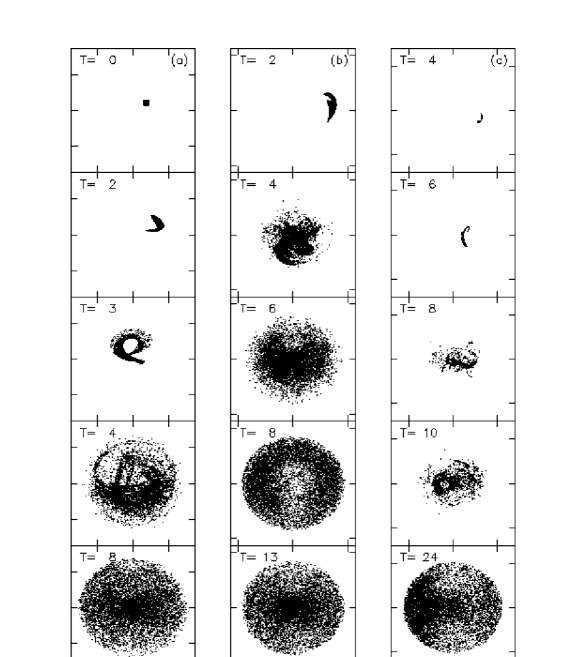
Figure 4: Mixing in a triaxial potential with a central point containing $3\%$ of the total mass. Time is in units of the local crossing time. Ensembles of $10^{4}$ phase points were distributed initially ($T=0$) in patches on an equipotential surface with zero velocity. Ensemble (a) was begun on a surface enclosing a mass $\sim 3$ times that of the “black hole”; for ensembles (b) and (c) these ratios were $\sim 7$ and $\sim 17$ respectively. Mixing occurs very rapidly for these ensembles, with a characteristic time of order the crossing time.

As stressed by Kandrup and co-workers ([Kandrup & Mahon 1994], [Kandrup 1990]), a useful way to think about the consequences of chaotic motion for the evolution of stellar systems is in terms of mixing. Mixing is the process by which an initially non-uniform distribution of points in phase space relaxes to a uniform one, at least in a coarse-grained sense ([Lichtenberg & Lieberman 1992]). It therefore provides a link between the behavior of individual orbits and the evolution of the phase-space density. While there are many discussions of mixing in the stellar dynamics literature ([Lynden-Bell 1967], [Tremaine et al. 1996], [Mathur 1988], [Soker 1996]), most of these are vague with regard the origin of the mixing or its properties. Kandrup et al. (1994) and Merritt & Valluri (1996) noted many of the special properties of chaotic mixing. It is irreversible, in the sense that an infinitely fine tuning is required to undo its effects. It has an associated time scale, the Liapunov time, in the sense that a compact set of points will initially separate at a rate determined by the Liapunov exponent. Following the arguments presented above, however, we expect mixing to produce significant changes in the macroscopic distribution of phase space points only if there are no barriers to the diffusion.

Figure 4 shows examples of chaotic mixing in a triaxial “imperfect ellipsoidal” potential ([Merritt & Valluri 1996]) with a shallow cusp and a central point mass. Three ensembles of orbits were started at rest on an equipotential surface and integrated in tandem for several crossing times. The central point had a mass $M_{h}=0.03$ (in units of the galaxy mass $M$), similar to the masses of the largest black holes observed in nearby galaxies ([Kormendy & Richstone 1995]). The first ensemble (a) was begun on an equipotential surface enclosing a mass $\sim 3$ times that of the “black hole”; for ensembles (b) and (c) these ratios were $\sim 7$ and $\sim 17$ respectively. The number in each frame is the elapsed time in units of the local crossing time. All ensembles were initially distributed in a tiny square patch as for $T=0$ in ensemble (a).

Mixing occurs very rapidly in these ensembles. At the lowest energy, (ensemble a), the linear extent of the points in configuration space doubles roughly every crossing time until $T\approx 4$, when the volume defined by the equipotential surface appears to be nearly filled. At the highest energy (ensemble c), mixing is slower but substantial changes still take place in a few crossing times. The final distribution of points at this energy still shows some structure, reminiscent of a box orbit.

Mixing in triaxial potentials with smaller central masses can be slower, requiring hundreds or even thousands of crossing times to reach a near-invariant state ([Merritt & Valluri 1996]) – even though the Liapunov exponents in these potentials are comparable (expressed in units of the local orbital frequency) to those of the orbits in Fig. 4. Here again, we find that Liapunov exponents are poor predictors of the rate of evolution.

The mixing illustrated in Fig. 4 takes place in a phase space that is globally chaotic, with almost no regular orbits. In triaxial potentials containing a central black hole, a “zone of chaos” extends from the nucleus out to a radius containing $\sim 10^{2}$ times the mass of the central point ([Merritt & Valluri 1999]). Each of the ensembles in Fig. 4 lies within this zone. Near the outer edge of the chaotic zone (ensemble c), the mixing is beginning to become non-random, and the distribution of points at the final time step still shows hints of structure. At still larger radii, or in potentials with smaller black holes, phase space is a complicated mixture of regular and chaotic trajectories (cf. Fig. 3) and mixing is correspondingly slower.

Mixing like that of Fig. 4 should produce rapid changes in the shape of a galaxy. Such evolution has in fact been observed in $N$-body simulations of the response of a triaxial galaxy to the growth of a central black hole. Merritt & Quinlan ([Merritt & Quinlan 1998]) found that a triaxial galaxy evolves to axisymmetry in little more than the local crossing time at each radius when the black hole mass exceeds $\sim 2.5\%$ of the total galaxy mass. There are two factors that can cause mixing at large radii to occur faster in these $N$-body simulations than in Fig. 4(c). First, in a self-consistent potential all orbits are initially well spread out and not confined to tiny patches as in the mixing experiments. Second, mixing timescales at small radii are almost 100 times faster (in absolute time units) than at the half mass radius. Once the inner region changes shape the orbits further out are no longer in equilibrium in the new potential and can respond more rapidly than they would in a fixed potential ([Barnes 1999]). Therefore the orbits at larger radii respond collectively both to the perturbing central black hole and to the potential changes at small radii. Smaller black holes induce slower evolution, consistent (at least qualitatively) with the less efficient mixing expected in such potentials ([Merritt & Valluri 1996]). Such experiments – which should be repeated with a wider range of initial conditions, including rotating models – confirm that chaos can be an important mechanism in determining the global structure of galaxies.

5 Conclusions

The orbits of stars in stellar systems are generically chaotic. Exponential sensitivity to perturbations implies that initially adjacent trajectories will diverge in a fraction of a crossing time. However this divergence does not necessarily imply a macroscopic evolution of the phase space distribution on a comparable time scale, as has been suggested by some authors. The reason is that perturbations may grow exponentially only for a limited time, saturating when separations are much smaller than the size of the system. This occurs, for instance, in a potential composed of $N$ point masses when $N$ is large. In such potentials, orbits can mimic regular orbits for many oscillations even though their Liapunov exponents are large. Only when perturbations are able to grow until their scale is of order the size of the system does the chaos have a significant influence on the macroscopic dynamics.

The redistribution of stars in phase space due to chaos may be simulated by mixing experiments in fixed potentials. Mixing leads to a near-invariant distribution of points within the accessible phase-space region. We find that mixing in a globally chaotic region of phase space – a region where almost all the orbits are stochastic – is very efficient, producing substantial changes in the distribution of points in just a crossing time. In phase space regions containing a mixture of regular and chaotic trajectories, mixing can be slower. The objects that impede mixing appear to be the resonant tori and their associated families of regular orbits. In triaxial potentials containing a central point mass, mixing becomes very efficient when the central mass is big enough to destroy all of the resonant tori. The result is large-scale evolution of the galaxy toward axisymmetric shapes.

References

- [Barnes 1999] Barnes, J. 1999,in Galaxy Dynamics, eds. D. Merritt, J. Sellwood, M. Valluri (ASP, San Francisco), 182, p. 463.
- [Binney & Spergel 1984] Binney, J. & Spergel, D. 1984, MNRAS, 206, 159.
- [Carpintero & Aguilar 1998] Carpintero, D. D. & Aguilar, L. A. 1998, MNRAS, 298, 1.
- [Chandrasekhar 1943] Chandrasekhar, S. 1943, Rev. Mod. Phys., 15, 1.
- [1993] Dehnen, W. 1993, MNRAS, 265, 250.
- [de Zeeuw 1985] de Zeeuw, P. T. 1985, MNRAS, 216, 273.
- [Gaspard 1998] Gaspard, P. 1998 Chaos, Scattering and Statistical Mechanics (Cambridge University Press, Cambridge).
- [Gerhard & Binney 1985] Gerhard, O. & Binney, J. J. 1985, MNRAS, 216, 467.
- [Goodman et al. 1993] Goodman, J., Heggie, D. C. & Hut, P. 1993, ApJ, 415, 715.
- [Gurzadyan & Savvidy 1986] Gurzadyan, V. G. & Savvidy, G. K. 1986, A&A, 160, 203.
- [Heggie 1991] Heggie, D., 1991, in Predictability, Stability, and Chaos in -Body Dynamical Systems, ed. A. E. Roy (Plenum Press, New York) p. 47.
- [Kandrup 1990] Kandrup, H. E. 1990, ApJ, 364, 420.
- [Kandrup & Mahon 1994] Kandrup, H. E. & Mahon, M. E. 1994, Phys. Rev. E, 49, 3735.
- [Kormendy & Richstone 1995] Kormendy, J. & Richstone, D. O. 1995, ARA&A, 33, 581.
- [Kandrup & Smith 1991] Kandrup, H. E. & Smith, H. 1991, ApJ, 374, 255.
- [Kuzmin 1973] Kuzmin, G. G. 1973, Dynamics of Galaxies and clusters Ed. T. B. Omarov, (Akad. Nauk. Kaz. SSR. Alma Ata., 71).
- [Laskar 1990] Laskar, J. 1990, Icarus, 88, 266.
- [Laskar et al. 1992] Laskar, J., Froeschlé, C. & Celletti, A. 1992, Physica D, 56, 253.
- [Laskar 1993] Laskar, J. 1993, Physica D, 67, 257.
- [Laskar 1998] Laskar, J. 1998, in NATO-ASI Hamiltonian systems with Three of More Degrees of Freedom, ed. C. Simo & A. Delshams (Kluwer, Dordrecht)
- [Lebowitz 1993] Lebowitz, J. L. 1993, Physica A, 194, 13.
- [Lichtenberg & Lieberman 1992] Lichtenberg, A.J. & Lieberman,M.A. 1992, Regular and Chaotic Motion (Springer, Berlin Springer).
- [Lynden-Bell 1967] Lynden-Bell, D. 1967, MNRAS, 136, 101.
- [Mathur 1988] Mathur, S. D. 1988, MNRAS, 231, 367.
- [Merritt & Valluri 1996] Merritt, D. & Valluri, M. 1996, ApJ, 506, 686.
- [Merritt & Quinlan 1998] Merritt, D. & Quinlan, G. 1998, ApJ, 498, 625.
- [Merritt & Valluri 1999] Merritt, D. & Valluri, M. 1999, AJ, 118, 1177.
- [Miller 1964] Miller, R. H.1964, ApJ, 140, 250.
- [1989] Miralda-Escudé, J. & Schwarzschild, M. 1989, ApJ, 339, 752.
- [1996] Papaphillipou, Y. & Laskar, J. 1996, A&A, 307, 427.
- [Papaphillipou & Laskar 1998] Papaphillipou, Y. & Laskar, J. 1998, A&A, 329, 451.
- [Soker 1996] Soker, N. 1996, ApJ, 457, 287.
- [Tremaine et al. 1996] Tremaine, S., Henon, M. & Lynden-Bell, D. 1986, MNRAS, 219, 285.
- [Valluri & Merritt 1998] Valluri, M. & Merritt, D. 1998, ApJ, 506, 686.
- [Valluri 1999] Valluri, M. 1999 in Galaxy Dynamics, eds. D. Merritt, J. Sellwood, M. Valluri (ASP, San Francisco) v. 182, p. 195.
- [Valluri & Merritt 1999b] Valluri, M. & Merritt, D. 1999, in Galaxy Dynamics, eds. D. Merritt, J.A. Sellwood & M. Valluri, (ASP, San Francisco) v. 182 p. 178.