Galaxies in Clusters: The Observational Characteristics of Bow-Shocks, Wakes and Tails

Abstract

The dynamical signatures of the interaction between galaxies in clusters and the intracluster medium (ICM) can potentially yield significant information about the structure and dynamical history of clusters. To develop our understanding of this phenomenon we present results from numerical modelling of the galaxy/ICM interaction, as the galaxy moves through the cluster. The simulations have been performed for a broad range, of ICM temperatures ($kT_{cl}=1$, 4 and $8\,\mbox{${\,\rm keV}$}$), representative of poor clusters or groups through to rich clusters.

There are several dynamical features that can be identified in these simulations; for supersonic galaxy motion, a leading bow-shock is present, and also a weak gravitationally focussed wake or tail behind the galaxy (analogous to Bondi-Hoyle accretion). For galaxies with higher mass-replenishment rates and a denser interstellar medium (ISM), the dominant feature is a dense ram-pressure stripped tail. In line with other simulations, we find that the ICM/galaxy ISM interaction can result in complex time-dependent dynamics, with ram-pressure stripping occurring in an episodic manner.

In order to facilitate this comparison between the observational consequences of dynamical studies and X-ray observations we have calculated synthetic X-ray flux and hardness maps from these simulations. These calculations predict that the ram-pressure stripped tail will usually be the most visible feature, though in nearby galaxies the bow-shock preceeding the galaxy should also be apparent in deeper X-ray observations. We briefly discuss these results and compare with X-ray observations of galaxies where there is evidence of such interactions.

1 Introduction

Most galaxies are not isolated (Tully 1987) but are members of groups or clusters which are gravitationally bound, though not necessarily virialised. Galaxies in such systems may experience a number of types of interaction with their environment: galaxy-galaxy encounters, which may trigger starbursts and can culminate in galaxy merging (Schweizer 1982), interaction with the potential of the system as a whole, which may for example, result in tidal stripping of loosely bound material from galaxy outskirts (Mamon 1987), and finally hydrodynamical interaction between the interstellar medium (ISM) in a galaxy, and any intergalactic gas trapped in the potential well of the galaxy system.

It is the last of these processes which is the subject of the present study. Interaction with the surrounding intracluster medium (ICM) may have a significant impact on the gas within a galaxy whenever it sweeps through a substantial mass of hot gas in its motion within a group or cluster. In practice, the hot ICM dominates the baryon content of galaxy clusters (White & Fabian 1995) and is also a major baryonic component within many galaxy groups (Mulchaey et al. 1996, Ponman et al. 1996).

The interaction between galaxies and the ICM should generate characteristic structures: at low galaxy velocities it will produce only a mild displacement of the outer regions of any gaseous galaxy halo, at higher velocities a bow shock should be generated ahead of the galaxy, and a wake of enhanced gas density may trail behind it.

These processes are important for three main reasons: first, gas may be removed from and/or accreted by the galaxy in such interactions with its gaseous environment, with important implications for subsequent galaxy evolution. Second, such processes will be responsible for some or all of the metals which are observed today within the ICM in clusters and groups, and may also affect the energetics of the ICM (Ponman, Cannon & Navarro 1999) – as such they are important for an understanding of the structure and evolution of galaxy systems. Finally, structures such as galaxy wakes provide information about the direction of motion of galaxies on the plane of the sky, which has in general been unavailable previously (Merrifield 1998). Given a good understanding of the astrophysics of the interaction, one may also be able to deduce the magnitude of the galaxy’s total velocity (allowing a full dynamical solution) and also to constrain the total mass of galaxies, including any dark halo.

Given the velocities of galaxies in groups and clusters, the temperature of the gas in shocks and wakes will be $\sim 10^{7}$ K, so the observational evidence of such processes is best sought at X-ray energies. To date shock and wake structures have only been observed in a few instances (detailed below), due to the limited sensitivity of existing X-ray telescopes. However, the improvements available from the upcoming X-ray observatories, Chandra and XMM  will enable detailed studies of structures around galaxies within clusters to be conducted. The aim of the present paper is to prepare for this, by exploring the astrophysics of the galaxy-ICM interaction using numerical hydrodynamic simulations, and in particular to investigate the observable properties of such interactions in the X-ray band.

The astrophysics is quite complex – several different mechanisms may be at work in any particular galaxy, and these will potentially have different signatures. Examples of such mechanisms include: i) a bow-shock, if the galaxy is moving supersonically through the ICM then there is the likelihood of a bow-shock preceeding the galaxy; ii) a gravitationally focussed wake, the mass and motion of the galaxy will tend to concentrate material behind it, in an analogous manner to Bondi-Hoyle accretion in binary systems (c.f. Hunt 1971); iii) ram pressure stripping of gas in the galaxy by the ICM will also result in a tail of enhanced density behind the galaxy. This feature, in the case of M86, has also been referred to as an X-ray plume (Rangarajan et al. 1995).

Examples of these features can be seen later in simulations of the galaxy/ICM interaction. While a bow-shock will be a distinct and recognisable feature, distinguishing between wakes (formed by gravitational focussing) and tails formed by stripping might be difficult on morphological grounds. In this paper we identify spectral as well as morphological signatures that can be used as a diagnostic of the physical mechanisms at work.

Currently there is only a limited amount of evidence of bow-shocks, wakes and tails around galaxies, observed primarily in relatively local systems. Some examples are:

1. White et al. (1991) reported on EINSTEIN observations of the Virgo galaxy M86, finding evidence for an X-ray plume, caused by ram pressure stripping as the galaxy moves through the cluster ICM. Rangarajan et al. (1995) analysed ROSAT observations of M86, finding that the X-ray plume, which they also interpret as being due to ram-pressure stripping, has a higher metallicity than either the cluster or M86 itself. The plume temperature is $kT=0.8\,\mbox{${\,\rm keV}$}$, similar to the galaxy emission from M86, but substantially lower than the cluster.

2. David et al. (1994) reported on ROSAT observations of a linear structure behind the dominant galaxy in the NGC 5044 group. they interpreted these results as being due to a “cooling wake” behind the galaxy, caused by motion of the galaxy with respect to the hot gas which follows the potential of the galaxy group.

3. Irwin & Sarazin (1996) reported on ROSAT HRI observations of the Virgo cluster elliptical galaxy NGC 4472, which shows a distorted X-ray morphology. Irwin & Sarazin (1996) suggested that this was strong evidence for a bow-shock like structure around the galaxy.

4. Sakelliou, Merrifield & McHardy (1996) reported on ROSAT results on observations of the wide-angled tail galaxy 4C 34.16 which lies in a poor cluster. Radio maps show two tails bent into a wide C-shape, and X-ray observations show an enhancement between the tails. Sakelliou et al. (1996) interpret this as due to motion of the galaxy through the ICM, and that this motion is responsible for both the jet bending and the X-ray wake trailing the galaxy.

5. The Fornax elliptical galaxy NGC 1404 shows an X-ray tail pointing away from the cluster centre, indicating that galaxy is infalling (Jones et al. 1997).

6. ROSAT observations of the Coma cluster found an elongated X-ray structure around the giant elliptical galaxy NGC 4839 (Dow & White 1995). NGC 4839 is probably the cD galaxy of a subcluster that is currently infalling into the main cluster. The X-ray tail of NGC 4839 is pointing away from the main cluster centre, supporting the infall idea.

7. H$\alpha$ observations of the edge-on spiral galaxy NGC 4388 by Veilleux et al. (1999) have found evidence of supersonic ram-pressure stripping. NGC 4388 is moving at $\sim 1500\mbox{${\,\rm km~{}s}^{-1}$}\,$ with respect to the ICM of the Virgo cluster, with a Mach number of ${\cal M}=3$. The X-ray emission from NGC 4388 is extended in the plane of the galaxy (Matt et al. 1994) but there is no evidence of X-ray extensions associated with ram-pressure stripping (though as Veilleux et al. (1999) point out, the galaxy orientation is unfavourable).

There have been a several papers considering the gas-dynamics of a galaxy moving through a cluster since the issue was considered by Gunn & Gott (1972). Shaviv & Salpeter (1982) reported on simulations, concentrating on the role of galaxy motion in ram-pressure stripping. Further simulations of the galaxy/ICM interaction have been presented by Takeda, Nulsen & Fabian (1984), who presented results of the dynamics of a galaxy moving radially through a cluster, suffering periodic stripping in the higher density regions near the centre of a cluster. Other studies of ram-pressure stripping have been presented by Nulsen (1982) and Portnoy, Pistinner & Shaviv (1993), as well as the work of Abadi, Moore & Bower (1999), which concentrates on the effect of ram-pressure stripping in clusters on the truncation of disks of spiral galaxies. The two most relevant papers to this work are those by Gaetz, Salpeter & Shaviv (1987) and Balsara, Livio & O’Dea (1994). Gaetz et al. (1987) presented a comprehensive study of ram-pressure stripping from galaxies, and calculated several important parameters affecting the efficiency of stripping. We shall use some of the parameters defined by Gaetz et al. (1987) in this paper. Balsara et al. (1994) present further calculations, using more sophisticated numerical techniques. Importantly, they found that the stripping process was much more complicated than seen in the calculations of Gaetz et al. (1987). When there was significant mass-replenishment of the ISM within the galaxy the resulting dynamical structure was complex, with material being stripped from the galaxy in long streamers from the edge of the galaxy, with the stripping happening is a discontinuous, episodic manner.

The calculations presented here represent an improvement over those of Gaetz et al. (1987) and Balsara et al. (1994) for the following reasons. The Gaetz et al. (1987) paper used a rather old numerical hydrodynamics code, which has substantial numerical viscosity. This has the effect of smearing out smaller scale features found in runs using more recent numerical hydrodynamic computer codes, such as the Piecewise Parabolic Method (PPM). This is important as in many runs the stripping process occurs in discrete events, with material being stripped of the edges of the galaxy. It is likely that in the Gaetz et al. (1987) models these processes were not be resolved. Balsara et al. (1994) used a more sophisticated code (PPM - essentially the same as used in this paper). However, Balsara et al. (1994) used a large value for the mass-replenishment rate ($\dot{M}_{rep}$). A large value of $\dot{M}_{rep}$ has the advantage of highlighting the complex dynamics of the galaxy/ICM interaction, but care has to be taken not to make it unrealistically large (see Section 2.3.3).

There are two further areas where this work is a significant improvement. First, from the simulations we calculate synthetic flux and hardness maps, as well as surface brightness profiles. These synthetic results can then be compared directly to actual observations of structures around galaxies in clusters. Such an approach will be necessary to fully understand the observed structures. Second, we perform a broad ranging parameter study, for parameters appropriate for a range of clusters, ranging from cool clusters or groups (with an ICM temperature of $kT_{cl}\sim 1\,\mbox{${\,\rm keV}$}$), up to hot clusters ($kT_{cl}\sim 8\,\mbox{${\,\rm keV}$}$).

The main purposes of this paper are twofold. First, to identify observational signatures of the galaxy/ICM interaction, which can be used in future detailed studies of individual objects, and second, to identify the circumstances in which galaxy/ICM interactions are most likely to be visible.

The paper is organised as follows: in Section 2 we discuss the hydrodynamical model used to investigate the phenomenon, including the model for the galaxy and the parameters used in the simulations. In Section 3 results from the simulations are presented and compared with analytic models of the galaxy/ICM interaction, in Section 4 the observable signatures of these simulations are discussed, and in Section 5 we discuss these results in the context of observations and conclude.

Table 1: The assumed parameters for the model clusters. The various symbols are defined in more depth in Section 2.2.

Parameter	Symbol (Units)	Cool Cluster	Intermediate Cluster	Hot Cluster
Cluster X-ray luminosity	$L_{x}$ (${\,\rm erg~{}s}^{-1}$ )	$6.1\times 10^{42}$	$2.8\times 10^{44}$	$1.9\times 10^{45}$
Cluster core radius	$R_{core}$ (kpc)	250	250	250
Velocity dispersion	$\sigma_{cl}$ (${\,\rm km~{}s}^{-1}$ )	371	795	1164
Cluster temperature	$kT_{cl}$ (keV)	1.0	4.0	8.0
Cluster sound speed	$a_{cl}$ (${\,\rm km~{}s}^{-1}$ )	520	1040	1460
Cluster density at galaxy radius1	$\rho_{cl}(R_{core})$ (${\,\rm gm\ cm}^{-3}$ )	$3.8\times 10^{-28}$	$2.5\times 10^{-27}$	$5.8\times 10^{-27}$
Central cluster surface brightness2	$S_{0}$ (${\,\rm erg~{}cm}^{-2}{\rm s}^{-1}{\rm arcmin}^{-2}$ )	$1.1\times 10^{-14}$	$5.1\times 10^{-13}$	$3.4\times 10^{-12}$

Notes for Table 1:

¹ In all simulations the galaxy is assumed to be at a radius of $r=R_{core}$ from the cluster centre.

² The quoted surface brightness is calculated assuming the cluster bolometric X-ray luminosity. The surface brightness in the ROSAT waveband will be correspondingly lower.

2 The Numerical Model

2.1 Introduction

To model the gas dynamics in and around a galaxy moving within a cluster we use the 2-D hydrodynamics code VH-1, which has been used extensively elsewhere in different contexts (Blondin et al. 1990; Stevens et al. 1992). The code uses the PPM algorithm and is good at resolving shocks in complex flows. It is basically very similar to that used by Balsara et al. (1994). The flow is assumed to be cylindrically symmetric.

In these simulations the gravitational effect of the galaxy on the ICM are included, as well as replenishment of the galaxy ISM by stellar populations. The parameters for both the galaxy and the clusters they are embedded in are described below.

2.2 The Model Galaxy Cluster

One of the main goals of this paper is to investigate the expected observational visibility of the galaxy/ICM interaction region. To do this we embed the results from the hydrodynamic simulations into a model cluster. We assume a spherical, isothermal cluster with a temperature $T_{cl}$ and cluster sound speed $a_{cl}$ (calculated assuming a mean mass per particle of $\bar{\mu}=10^{-24}$ gm). Simulations for three different values of $T_{cl}$; a) $T_{cl}=1\,\mbox{${\,\rm keV}$}$ have been performed, representative of a poor cluster, such as Fornax (c.f. 4C 34.16, Sakelliou et al. 1996), b) $T_{cl}=4\,\mbox{${\,\rm keV}$}$, representative of a more substantial cluster, such as Abell 1060 or AWM 7 (both of which have temperatures $\sim 4\,\mbox{${\,\rm keV}$}$; Loewenstein & Mushotzky 1996), and c) $T_{cl}=8\,\mbox{${\,\rm keV}$}$, indicative of a rich cluster such as Coma.

We assume the following scaling relationships for the cluster X-ray luminosity ($L_{x}$) and velocity dispersion ($\sigma_{cl}$, White, Jones & Forman 1997):

$$L_{x}(\mbox{${\,\rm erg~{}s}^{-1}$\,})=6.1\times 10^{42}\left(kT_{cl}\right)^{2.77}$$ (1)

$$\sigma_{cl}(\mbox{${\,\rm km~{}s}^{-1}$}\,)=371\left(kT_{cl}\right)^{0.55}$$ (2)

with $kT_{cl}$ in  ${\,\rm keV}$. For the model clusters a $\beta=2/3$ mass distribution has been assumed (see below). The X-ray luminosity given by eqn. (1) is the total bolometric X-ray luminosity, rather than the ROSAT luminosity. A cluster core radius of $R_{core}=250$ kpc and a distance of $D=50$ Mpc is assumed for all clusters (c.f. Jones & Forman 1984).

Future studies of individual galaxies in clusters will be able to use values of $L_{x}$ (and $\beta$ and $\sigma_{cl}$ etc) appropriate for the cluster in question. However, these scaling relationships are adequate for a general study of the observational characteristics of structures around galaxies. For simplicity, the galaxy is assumed to be moving through material of constant density, at a distance of $r=R_{core}$ from the cluster centre.

For $\beta=2/3$, the surface brightness distribution $S(w)$ of the model cluster as a function of projected distance from the cluster centre $w$ is

$$S(w)=\frac{S_{0}}{\left(1+(w/R_{core})^{2}\right)^{3/2}}\ ,$$ (3)

where $R_{core}$ is the cluster core radius, and $S_{0}$ is the central surface brightness. This profile integrates to give the a total X-ray luminosity of $L_{x}=8\pi^{2}S_{0}R_{core}^{2}$. Also, for $\beta=2/3$, the gas density profile within the cluster $\rho_{c}l(r)$ varies as

$$\rho_{cl}(r)=\frac{\rho_{cl}(0)}{\left(1+(r/R_{core})^{2}\right)}$$ (4)

with $\rho_{cl}(0)$ the cluster central gas density. At $r=R_{core}$ the gas density $\rho_{cl}(R_{core})=\rho_{cl}(0)/2$. Details of the parameters for the model clusters are given in Table 1.

2.3 The Model Galaxy

2.3.1 Mass Distribution

The parameters for the model galaxy used here are similar to those of Gaetz et al. (1987). The galaxy is assumed to be spherical, with the mass in the galaxy dominated by stars. The stellar density distribution within the galaxy is given by

$$\rho_{\ast}(r)=\frac{\rho_{\ast}(0)}{\left(1+(r/R_{c})^{2}\right)}\ ,$$ (5)

with $R_{c}$ the core radius of the mass distribution ($R_{c}=1.5$ kpc in these simulations), and $\rho_{\ast}(0)$ is the central density in the galaxy. We assume that the mass distribution of the galaxy extends out to a radius $R_{H}=32.2$ kpc (Balsara et al. 1994). The total galaxy mass, $M_{gal}$, is then

$$M_{gal}=4\pi\rho_{\ast}(0)R_{c}^{3}\left[\frac{R_{H}}{R_{c}}-\tan^{-1}\left(\frac{R_{H}}{R_{c}}\right)\right]\ .$$ (6)

In these simulations $M_{gal}=1.2\times 10^{12}\mbox{\,$M_{\odot}$\,}$, which then specifies the galaxy central stellar density $\rho_{\ast}(0)$. The assumed parameters for the model galaxy are summarised in Table 2.

2.3.2 Galaxy Velocity

For a galaxy cluster with a one-dimensional velocity dispersion of $\sigma_{cl}$ the mean galaxy velocity will be $V_{mean}=\sqrt{3}\sigma_{cl}$. The model galaxy is assumed to be moving at a velocity $V_{gal}$ through the ICM, and for each of the three model clusters simulations with two values of $V_{gal}$, have been run, with $V_{gal}=1.0$ or $1.5V_{mean}$. The relationship between $\sigma_{cl}$ and cluster temperature (eqn. 2) means that $V_{gal}\propto kT_{cl}^{0.55}$.

For these values of $V_{gal}$ all the model galaxies are moving supersonically, with Mach numbers ${\cal M}=1.2-2.1$. This range of values should be representative, though some galaxies of interest have even higher Mach numbers (c.f. NGC 4388, Veilleux et al. 1999). The steeper dependence of $V_{gal}$ on $T_{cl}$ compared to the sound speed, means that the galaxies in clusters with higher $kT_{cl}$ have marginally higher Mach numbers. Details of the velocities for the different models are in Table 3.

Table 2: Parameters for the model galaxy used in all the simulations. The symbols used are defined in more depth in Section 2.3.

Parameter	Symbol	Value
Galaxy mass	$M_{gal}$	$1.2\times 10^{12}\mbox{\,$M_{\odot}$\,}$
Galaxy central stellar density	$\rho_{\ast}(0)$	$9.48\times 10^{-23}\mbox{${\,\rm gm\ cm}^{-3}$\,}$
Galaxy core radius	$R_{c}$	1.5 kpc
Galaxy outer radius	$R_{H}$	32.2 kpc
Mass replenishment half-radius	$R_{0}$	8.7 kpc
Mass replenishment outer radius	$R_{rep}$	15.5 kpc
Mass replenishment temperature	$T_{rep}$	$1.87\times 10^{6}$ K
Star formation density threshold	$\rho_{sf}$	$2.34\times 10^{-24}\mbox{${\,\rm gm\ cm}^{-3}$\,}$
Star formation temperature threshold	$T_{sf}$	$2.0\times 10^{4}$ K
Star formation timescale	$\tau_{sf}$	$3.25\times 10^{7}$ yr

2.3.3 Mass replenishment within the galaxy

In galaxies a combination of stellar mass loss and supernovae act to continuously replenish the gas within the galaxy. This mass-replenishment will affect the flow around the galaxy in several ways. First, it provides material that can be continuously stripped and second, it acts as barrier (if dense enough) to the ICM, resulting in the formation of a bow-shock preceeding the galaxy. In these simulations the radial distribution of the mass replenishment is assumed to have basically the same form as that of the stellar distribution, that is

$$\dot{\rho}_{rep}(r)=\frac{\dot{\rho}_{rep}(0)}{\left(1+(r/R_{c})^{2}\right)}$$ (7)

for $r\leq R_{rep}$, where $R_{rep}$ is the outer radius for mass-replenishment. The characteristic radius $R_{0}$ is the mass replenishment half-radius - half of the mass-replenishment occurs inside a radius $R_{0}$. This prescription is equivalent to “Case 1” in Gaetz et al. (1987).

This expression can be integrated to give an expression for the total mass-injection rate within the galaxy

$$\dot{M}_{rep}=4\pi{\dot{\rho}_{rep}(0)}R_{c}^{3}\left[\frac{R_{rep}}{R_{c}}-\tan^{-1}\left(\frac{R_{rep}}{R_{c}}\right)\right]\ .$$ (8)

The value of $\dot{\rho}_{rep}(0)$ is determined by the assumed total rate of mass injection into the galaxy $\dot{M}_{rep}$. Assuming a galactic mass/light ratio of 20 (in solar units) gives $L=5\times 10^{10}\mbox{\,$L_{\odot}$\,}$ for the model galaxy. This mass/light ratio implies a modest dark matter halo. Faber & Gallagher (1976) estimated that the rate of mass-replenishment into an elliptical galaxy was $0.015\mbox{\,$M_{\odot}$\ {\rm yr}${}^{-1}$\,}\times(10^{9}\mbox{\,$L_{\odot}$\,})$, so the expected mass-replenishment rate for a $1.2\times 10^{12}\mbox{\,$M_{\odot}$\,}$ galaxy is $\sim 1\mbox{\,$M_{\odot}$\ {\rm yr}${}^{-1}$\,}$. As discussed by Gaetz et al. (1987), the relationship of Faber & Gallagher (1976) was estimated assuming a single coeval populations of stars, with a current main sequence turn-off mass of $1\mbox{\,$M_{\odot}$\,}$. Younger populations of stars will enhance the mass-replenishment rate, and so the value of $1\mbox{\,$M_{\odot}$\ {\rm yr}${}^{-1}$\,}$ should be considered as a lower limit. The results of Mathews (1989) suggest a value of $\dot{M}_{rep}=5\mbox{\,$M_{\odot}$\ {\rm yr}${}^{-1}$\,}$ as a reasonable upper limit, when there is mass-replenishment from a younger stellar population. Consequently, two sets of simulations with $\dot{M}_{rep}=1\mbox{\,$M_{\odot}$\ {\rm yr}${}^{-1}$\,}$ and $5\mbox{\,$M_{\odot}$\ {\rm yr}${}^{-1}$\,}$ have been calculated. The temperature of the replenished gas is assumed to be $T_{rep}=1.87\times 10^{6}$ K, the same as in Balsara et al. (1994) and Gaetz et al. (1987).

We note that Balsara et al. (1994) used a rather high value of the mass-replenishment rate ($\sim 15\mbox{\,$M_{\odot}$\ {\rm yr}${}^{-1}$\,}$). Such a large value leads automatically to the formation of dense structures in the centre of the galaxy. However, even with lower values of $\dot{M}_{rep}$, under some circumstances, dense and complex structures are formed within the galaxy.

2.3.4 Star-formation

In several of the simulations presented in Section 3 a considerable amount of cold, dense gas accumulates in the centre of the galaxy. We include the possibility of star-formation in the simulations, in an identical way to Balsara et al. (1994), which is essentially as a mass-sink in the centre of the galaxy. No feedback mechanisms (i.e. the formation of a young stellar population leading to an increase in the mass-replenishment rate) is included. Such refinements could be easily included in more sophisticated models.

As implemented here the action of star-formation is to remove gas from the central regions of the galaxy. Material is assumed to form stars or molecular clouds and effectively drops out of the hydrodynamic equations. When star-formation does occur the rate of change of gas density is given by;

$$\dot{\rho}_{sf} = -\frac{\rho}{4\tau_{sf}}\left(1+\tanh\left[\frac{\rho-\rho_{sf}}{0.1\rho_{sf}}\right]\right)$$ (9)

$$\times\left(1+\tanh\left[\frac{T_{sf}-T}{0.1T_{sf}}\right]\right)$$

In this equation $\rho_{sf}$ and $T_{sf}$ are the effective density and temperature thresholds above which and below which star-formation will occur. The star-formation time-scale $\tau_{sf}$ specifies the time-scale on which the star-formation occurs. In these simulations $\rho_{sf}=2.4\times 10^{-24}\mbox{${\,\rm gm\ cm}^{-3}$\,}$, $T_{sf}=20000$K, and $\tau_{sf}=3\times 10^{7}$ years.

In our simulations star-formation only occurs in a subset of the runs (see Section 3), and when it does occur it only happens in the innermost regions of the galaxy. Star-formation, as implemented here, does not have any substantial effect on the flow-properties outside of these inner regions, but it does prevent the densities in the central region of the galaxy growing, unchecked, to unphysical levels.

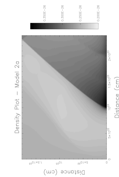
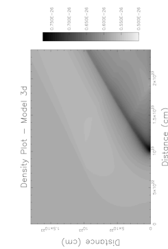
Figure 1: The density and temperature structure for two simulations that show the “Efficient Stripping” (ES) behaviour. Upper panels - results for Model 2a (4 ${\,\rm keV}$ cluster - low velocity and low mass-replenishment rate). Note the bow-shock structure, and also the relatively small mass density/temperature perturbations associated with the galaxy. Lower panels - results for Model 3d (8 ${\,\rm keV}$ cluster - high velocity and high mass-replenishment). The bow shock is visible and has a smaller opening angle due to the higher Mach number of the flow.

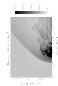
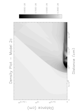
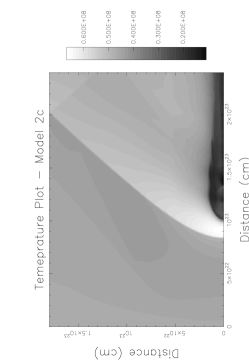
Figure 2: The density and temperature structure for two simulations for the “Mass-Retention” (MR) mode. Upper panels - results for Model 1b (1 ${\,\rm keV}$ cluster, low velocity, high mass-replenishment rate). Note the strong density enhancements in the form of streamers in the tail region. There is a considerable amount of cool and dense gas at the centre of the galaxy. Lower panels - results for Model 2c (4 ${\,\rm keV}$ cluster, low velocity, high mass-replenishment rate). The bow shock is again clearly visible as well as a dense tail behind the galaxy caused by ram-pressure stripping. The tail is not as over dense as for the case in the top-panels, and is smaller in extent.

2.4 Description of Simulations

A total of 12 simulations have been run, four each for the cool, intermediate and hot clusters, with two values for the galaxy velocity and mass-replenishment rate. Details of the parameters for each model are given in Table 3. The simulations were all run on a $240\times 180$ 2-D cylindrical grid, with an extent of $2.4\times 10^{23}$ cm by $1.8\times 10^{23}$ cm ($\sim 80\times 60$ kpc). At an assumed cluster distance of 50 Mpc each cell corresponds to an angular extent of 1.3 arcsec.

2.5 Useful Parameters

Gaetz et al. (1987) introduced some parameters and timescales that are useful to characterise these simulations. The flow-crossing timescale is defined as

$$\tau_{flow}=\frac{2R_{0}}{V_{gal}}\ .$$ (10)

For the range of velocities considered $\tau_{flow}$ is in the range $(0.6-2.6)\times 10^{7}$ yr. The characteristic orbital timescale within the galaxy is defined as

$$\tau_{orb}=\frac{2\pi R_{0}}{v_{circ,0}}$$ (11)

with

$$v_{circ,0}=\left(\frac{GM(R_{0})}{R_{0}}\right)^{1/2}$$ (12)

with $M(R_{0})$ the total mass-contained within a radius $R_{0}$. For the model galaxy $M(R_{0})=2.6\times 10^{11}\mbox{\,$M_{\odot}$\,}$, so that $v_{circ,0}=360\mbox{${\,\rm km~{}s}^{-1}$}\,$, and $\tau_{orb}=4.7\times 10^{7}$ yr.

An important quantity in these simulations will be the fraction of mass retained by the galaxy in the gas-phase and the amount of gas ram-pressure stripped from the galaxy. Gaetz et al. (1987) parameterised the fraction of mass ram-pressure stripped from the galaxy using two parameters, $\nu$ and $\omega$, where

$$\nu=\frac{\pi R_{0}^{2}\rho_{cl}V_{gal}}{\dot{M}_{rep}}\ ,$$ (13)

with $\rho_{cl}$ the ICM density and

$$\omega=4\left(\frac{V_{gal}}{10^{3}\mbox{${\,\rm km~{}s}^{-1}$}\,}\right)^{2}\left(\frac{v_{esc,0}}{500\mbox{${\,\rm km~{}s}^{-1}$}\,}\right)^{-2}\ .$$ (14)

The escape velocity from the galaxy at a radius $R_{0}$ is

$$v_{esc,0}=\left(2|\phi(R_{0})-\phi(\infty)|\right)^{1/2}\ .$$ (15)

with $\phi$ the gravitational potential. For the parameters used here $v_{esc,0}=850\mbox{${\,\rm km~{}s}^{-1}$}\,$ (Table 2).

The parameter $\nu$ is the ratio of the external to internal mass-flow rate into the galaxy, and $\omega$ a dimensionless measure of galaxy velocity. With these two parameters Gaetz et al. (1987) defined a dimensionless stripping parameter $\xi=\nu\omega^{0.7}$ that related directly to the fraction of mass-stripped from the galaxy (their Fig. 3). Consequently, the rate of ram-pressure stripping is $\propto\rho_{cl}V_{gal}^{2.4}$.

From the simulations we calculate the fraction of the replenished gas that is retained by the galaxy ($\Phi$). We estimate the mass of gas $M_{gas}$ within a radius $R_{0}$ at two times $t_{1}$ and $t_{2}$, with $t_{1}$ and $t_{2}$ chosen to lie at times where the solution has settled down to a steady state (or at least a quasi-steady state - see Section 3.2). We then define $\Phi$ as:

$$\Phi=\frac{\left[M_{gas}(t_{2})-M_{gas}(t_{1})\right]+\left[M_{sf}(t_{2})-M_{sf}(t_{1})\right]}{(t_{2}-t_{1})\dot{M}_{rep}}\ ,$$ (16)

where $M_{sf}(t)$ is the total mass removed from the system by star-formation up to a time $t$. From their models, Gaetz et al. (1987) empirically found that $\Phi$ could be represented by the following expression

$$\Phi=\left(1+\left(\frac{\xi}{\xi_{1/2}}\right)^{1.23}\right)^{-1}$$ (17)

with $\xi_{1/2}=0.6$ is the value of $\xi$ at which $\Phi=0.5$. Our results for $\Phi$ will be discussed in Section 3.

Other parameters from the simulations that will be useful for comparison with observations are the emission weighted temperatures of specified regions within the simulations. For all of the simulations we have calculated the emission weighted temperature for two regions. The first covers the galaxy itself, and comprises a sphere, radius $R_{0}$, centred on the galaxy ($\bar{T}_{gal}$). The second covers the tail region, and is a cylinder, radius $R_{0}$, extending from a distance $R_{0}$ behind the galaxy to the edge of the grid $(\bar{T}_{tail}$). The emission weighted temperature $\bar{T}$ is defined as

$$\bar{T}=\frac{\sum_{cells}n^{2}\Lambda(T)T}{\sum_{cells}n^{2}\Lambda(T)}$$ (18)

with $n$ the gas number density and $\Lambda(T)$ the emissivity of the gas. The summation is carried out over all cells within the region of interest. The values of $\bar{T}_{gal}$ and $\bar{T}_{tail}$ for each of the simulations are shown in Table 3, although it should be noted that because some of the simulations never settle down to a steady state, the values of $\bar{T}_{tail}$ and $\bar{T}_{gal}$ can vary with time.

Table 3: The assumed and derived parameters for the simulations.

		$V_{gal}$	$\dot{M}_{rep}$	${\cal M}$	$\xi$	$\Phi$	$\bar{T}_{gal}$	$\bar{T}_{tail}$	Mode
		(${\,\rm km~{}s}^{-1}$ )	( $M_{\odot}$ yr-1 )				(K)	(K)
		(1)	(2)	(3)	(4)	(5)	(6)	(7)	(8)
Cool cluster models ($kT_{cl}=1\,\mbox{${\,\rm keV}$}=1.2\times 10^{7}$K)
	Model 1a	640	1.0	1.2	0.59	0.33	$1.2\times 10^{5}$	$1.1\times 10^{7}$	MR
	Model 1b	960	1.0	1.9	1.6	0.31	$3.5\times 10^{4}$	$1.1\times 10^{7}$	MR
	Model 1c	640	5.0	1.2	0.12	0.89	$2.4\times 10^{4}$	$1.1\times 10^{7}$	MR
	Model 1d	960	5.0	1.9	0.31	0.75	$1.3\times 10^{4}$	$1.1\times 10^{7}$	MR
Intermediate cluster models ($kT_{cl}=4\,\mbox{${\,\rm keV}$}=4.6\times 10^{7}$K)
	Model 2a	1380	1.0	1.3	24.7	0.0	$5.1\times 10^{7}$	$5.1\times 10^{7}$	ES
	Model 2b	2070	1.0	2.0	65.5	0.0	$4.8\times 10^{7}$	$5.2\times 10^{7}$	ES
	Model 2c	1380	5.0	1.3	4.9	0.03	$5.2\times 10^{7}$	$2.9\times 10^{7}$	MR
	Model 2d	2070	5.0	2.0	13.1	0.0	$5.6\times 10^{7}$	$4.9\times 10^{7}$	ES
Hot cluster models ($kT_{cl}=8\,\mbox{${\,\rm keV}$}=9.3\times 10^{7}$K)
	Model 3a	2010	1.0	1.4	141.5	0.0	$9.5\times 10^{7}$	$9.7\times 10^{7}$	ES
	Model 3b	3015	1.0	2.1	374.5	0.0	$9.4\times 10^{7}$	$9.8\times 10^{7}$	ES
	Model 3c	2010	5.0	1.4	28.3	0.0	$9.9\times 10^{7}$	$9.3\times 10^{7}$	ES
	Model 3d	3015	5.0	2.1	74.9	0.0	$9.8\times 10^{7}$	$9.8\times 10^{7}$	ES

Notes on Table 3

Column (1): Galaxy velocity with respect to the cluster ICM (Section 2.3.2).

Column (2): Galaxy mass-replenishment rate (Section 2.3.3).

Column (3): The Mach number of the galaxy with respect to the undisturbed ICM.

Column (4): The ram-pressure stripping parameter (Section 2.5).

Column (5): The galaxy mass-retention fraction (eqn. 16).

Columns (6) and (7): The mean temperatures in the tail region and galaxy centre region (Section 2.5).

Column (8): The mode of stripping for this model: ES - “Efficient Stripping”; MR - “Mass-Retention” (see Section 3 for an explanation).

3 Results

In this section we discuss the basic dynamical features found in these simulations. In Section 4 we go on to discuss the expected observable features that may be seen at X-ray energies.

There are two basic dynamical modes of behaviour in these simulations (illustrated in Figs. 1 and 2). The first is when the galaxy is completely stripped by the ICM (and the mass-retention fraction $\Phi\sim 0$), and there is no substantial build up of material at the galaxy centre. We term this flow behaviour the “Efficient Stripping” or ES mode. The second is when there is a substantial build up of material in the centre of the galaxy, and the stripping is less efficient ($\Phi\sim 0.1-0.6$). We term this flow behaviour the “Mass-Retention” or MR mode. In the first case the dynamics are relatively simple, while for the second case the dynamics are complex, resulting in a chaotic downstream region. Results from simulations showing both forms of behaviour are shown in Figs. 1 and 2. For each of the model runs listed in Table 3 the main dynamical mode is identified. As discussed later, however, the distinction between the modes is not always completely clear cut.

3.1 The “Efficient Stripping” Mode

We illustrate the case of the “Efficient Stripping” mode by looking, in detail, at two representative simulations, one each for the intermediate and hot cluster models (Models 2a and 3d). The density and temperature structure for both models are shown in Fig. 1.

Consider Model 2a first. This is a lower Mach number simulation, with ${\cal M}=1.3$. The density and temperature structure, at a time $5\times 10^{8}$ yr into the run, are shown in the top panels of Fig. 1. The basic flow structure is relatively simple and the simulation quickly settles down quickly to a steady state. The main features that can be seen in Fig. 1 are as follows:

1. a prominent bow-shock in front of the galaxy, visible in both the density and temperature plot. There is an increase in density and temperature across the shock. The peak post-shock temperature is $5.7\times 10^{7}$ K, compared to the ambient ICM temperature of $4.6\times 10^{7}$ K (Fig. 3). This increase in temperature is that given by the Rankine-Hugoniot conditions for a shock transition with this Mach number.

2. The gravitational acceleration of the ICM material by the galaxy results in a lower density region preceeding the galaxy.

3. There is little material accumulated at the centre of the galaxy, with a peak density of $\rho=4\times 10^{-27}\mbox{${\,\rm gm\ cm}^{-3}$\,}$ (Fig. 3). The density never gets high enough for star-formation to occur. In contrast, the peak density can be much higher in simulations with a higher $\dot{M}_{rep}$.

4. The galaxy is completely ram-pressure stripped, with the mass-retention fraction $\Phi\sim 0$.

5. On account of the relatively small perturbations in density and temperature the values of $\bar{T}_{gal}$ and $\bar{T}_{tail}$ are similar to the ambient cluster temperature.

6. The ICM velocity field is not greatly affected by the galaxy. Material in front of the galaxy is gravitationally accelerated, then decelerated both by the shock and by the mass-loading of replenished material, which is swept straight out of the galaxy. There are no regions where there is a region of downstream reverse flow back in the galaxy (c.f. Fig. 4).

The results for Model 3d (shown in the lower panel of Fig. 1), are essentially the same as for Model 2a. The results are shown at a time $2.5\times 10^{8}$ yr after the start of the simulation. In spite of the fact that the mass-replenishment rate for this simulation is higher than for Model 2a the ram-pressure of the cluster is still sufficient to completely strip the galaxy. From Fig. 1, for Model 3d the opening angle of the bow-shock is substantially smaller. This is due to the higher Mach number of the flow (${\cal M}=2.1$) for Model 3d compared to ${\cal M}=1.3$ for Model 2a.

The expected observational signatures for these simulations will be discussed in Section 4.

Figure 3: Left panel: The density profiles along the $x$-axis for the four simulations shown in Figs. 1 and Fig. 2. Shown are results for Model 1b (solid line), Model 2a (dotted line), Model 2c (dashed line) and Model 3d (dot-dashed line). Note, that the cluster ambient density is function of cluster temperature, with the hottest cluster having the highest ambient density. There is a clear difference between these simulations, with ES mode simulations (Models 2a and 3d) showing little density enhancements, while MR mode simulations (Models 1b and 2c) show pronounced density enhancements in both the galaxy region and the downstream region. In particular, the double shock structure, discussed by Balsara et al. (1994), is visible for Model 1b (solid line). Right Panel: The temperature profiles along the $x$-axis. The lines as the same as in the left panel. The ES mode simulations show only small temperature perturbations, while MR mode simulations show more complex structure.

3.2 The “Mass-Retention” Mode

In contrast to the relatively simple dynamics for the “Efficient Stripping” cases described above, when the mass-replenishment is sufficient or the ram-pressure low enough, complex and time-dependent flow patterns result in the vicinity of the galaxy. In these cases, material accumulates in the central region of the galaxy and dense blobs and streams of material are stripped from the galaxy. In this situation we do expect to see observable consequences of the galaxy/ICM interaction.

The MR mode is illustrated in Fig. 2 with results from two simulations (Model 1b, top panels and Model 2c, bottom panels), and we will concentrate on Model 1b initially. The density and temperature profiles shown in Fig. 3 are at a time $6.8\times 10^{8}$ yr after the start of the simulation. The MR simulations typically do not settle down to a steady-state, as there is a radial “pumping”mode instability in the flow (as discovered and discussed by Balsara et al. 1994). However, the MR mode simulations do reach a broadly quasi-steady state configuration.

As in the case of “Efficient Stripping” a large bow-shock region leading and enveloping the galaxy is apparent, caused by the interaction of ICM with the galaxy. As noted earlier we also a leading bow-shock in the case when efficient stripping occurs. In this case the opening angle of the bow-shock is broadened by the accumulated replenished material at the centre of the galaxy. Behind the bow-shock is a region of shock heated gas (though the temperature enhancements is small given the relatively low Mach number of the flow).

However, the main difference between this simulation and Model 2a shown in Fig. 1 is the complex structure around the galaxy. There is also a dense region at the galaxy centre, with ram pressure stripping primarily occurring from the outer layers of the galaxy. Complex Kelvin-Helmholtz type instabilities develop at the boundary where stripping is occurring. The stripping events result in long-dense filamentary structures trailing the galaxy. A consequence of this stripping is the formation of a dense, potentially observable, tail (Section 4).

For Model 1b, within the outer bow-shock is a second shock, resulting from the inflow from material from the downstream region passing through the galaxy (and being mass-loaded by the galactic mass-replenishment) before interacting with the incident ICM. The density profile for Model 1b is shown in Fig. 3, and shows both shocks. The formation of this second shock is discussed in Balsara et al. (1994).

In Model 1b the ram-pressure stripping is sporadic, with large amounts of material being stripped over short timescales. These mass-stripping events occurs on a time scale of a few times the flow-crossing timescale, $\tau_{flow}$.

To further illustrate the complex flow dynamics for Model 1b in Fig. 4 we show the $x$ component of the velocity at four different locations in the flow. In the undisturbed region ahead of the galaxy and bow-shock the gas velocity is essentially constant with time. At the galaxy centre there is sufficient build up of material to ensure that any velocities are small. There are, however, velocity excursions with both positive and negative values. The most interesting flow pattern is behind the galaxy, where the flow is complex, with periods of flow into the galaxy from the downstream region. Apparent from Fig. 4 the timescale for these events is $\sim 5\times 10^{7}$ years, a few times $\tau_{flow}$. This is instability behaviour noted by Balsara et al. (1994).

For the case of Model 2c, the basic density and temperature pattern is broadly similar to that for Model 1b (Fig. 3), in that there is a bow-shock and an enhanced density tail. However, Model 2c is a less extreme case than Model 1b, with the enhancement in density at the centre of the galaxy being only a factor of a few rather than several orders of magnitude. The tail is also narrower and shows less complex structure. Model 2c seems to be close to the transition between the ES and MR mode. At earlier times in the simulation it more closely resembles the ES case, but as the simulation progressed the velocity at the centre of the galaxy dropped with progressive mass-loading. Mass accumulates at the centre, making it more difficult to strip the galaxy (and so on). This simulation illustrates that the distinction between the two modes of behaviour is not completely clear cut, and in particular as the environment of the galaxy changes (as it moves closer or further from the galaxy centre) then the dynamics will also change. So, for example, while all runs for the hot cluster in Table 3 show the ES mode, even with the high mass-replenishment rate, if the galaxy were at a larger radius from the cluster centre then, because the cluster ram-pressure is lower, the galaxy would be able to retain much of the replenished mass, and the dynamics would be very different (see Section 3.3). It will also be possible for the flow pattern to undergo the opposite transition. Consider a situation like Model 1b, with the galaxy losing mass by discontinuous stripping events. If the incident ICM ram-pressure were to increase (either higher density or higher velocity), as might be expected if a galaxy was falling into the centre of a galaxy cluster, at some point the ram pressure would be sufficient to completely strip the galaxy, and the galaxy would return to the efficient continuous stripping mode. Calculations by Takeda et al. (1984) suggest that this transition can happen very rapidly, with the expulsion of a dense blobs of gas from the centre of the galaxy.

Figure 4: The time-variation of the $x$-component of the gas velocity with respect to the galaxy at several points in the flow for Model 1b. The sampling positions are at $x=10^{22}$ cm (i.e. well in front of the galaxy - dot-dashed line), $x=9\times 10^{22}$ cm (i.e. a small distance in front of the galaxy centre - dotted line), $10^{23}$ cm (at the galaxy centre - dashed line), and $1.5\times 10^{23}$ cm (behind the galaxy - solid line). Behind the galaxy the $x$-component of the velocity changes sign several times in a quasi-periodic manner, implying back-flow into the galaxy, which results in the build-up of material at the centre of the galaxy. This is the ‘pumping mode’ instability discussed in Balsara et al. (1994).

Figure 5: The mass retention fraction $\Phi$ versus the mass-stripping parameter $\xi$. The points are the results from the simulations presented here and the line is the best fit to the results of Gaetz et al. (1987; eqn. 17).

3.3 General Considerations

Although we have characterised the behaviour of the simulations presented here into two broad classes, the ES and MR modes, in reality the distinction is not always clear cut, as illustrated by Model 2c.

In Fig. 5 we plot the mass-retention fraction ($\Phi$) versus the ram-pressure stripping parameter ($\xi$) as defined by Gaetz et al. (1987). The best-fit model for the Gaetz et al. (1987) simulations is also shown (eqn. 17). The results of our simulations are similar to those of Gaetz et al. (1987), and broadly speaking the transition from the MR mode to the ES mode occurs for values of $\xi\sim 5-10$.

Consideration of Fig. 2 and the simulations presented in Balsara et al. (1994) shows that for the MR mode material accumulates in the center of the galaxy, and ram-pressure stripping occurs from the outer edges of this denser central region. So, even while a galaxy may retain mass at its centre, beyond a certain radius it will be completely stripped. Using the results of Takeda et al. (1984) we can evaluate the conditions from ram-pressure stripping at different radii within the galaxy.

Takeda et al. (1984) found that for a spherical galaxy, the ISM will be stripped from a galaxy at a projected radius $d$ when

$$\rho_{cl}V_{gal}^{3}\geq{C\alpha_{\ast}\Sigma_{\ast}(d)\sigma_{\ast}^{2}}\ ,$$ (19)

where $\rho_{cl}$ is the density of the incident ICM, $V_{gal}$ is the galaxy velocity, $\alpha_{\ast}$ is the fraction of the stellar mass injected into the galaxy ISM (i.e. for $\dot{M}_{rep}=1\mbox{\,$M_{\odot}$\ {\rm yr}${}^{-1}$\,}$, $\alpha_{\ast}=2.6\times 10^{-20}$ s^-1), $\Sigma_{\ast}(d)$ is the stellar surface density at a projected radius $d$, $\sigma_{\ast}$ the stellar velocity dispersion, and $C$ a constant to be empirically determined. For $M_{gal}\sim 10^{12}\mbox{\,$M_{\odot}$\,}$ a reasonable value is $\sigma_{\ast}=320\mbox{${\,\rm km~{}s}^{-1}$}\,$ (c.f. Djorgovski & Davis 1987).

From the stellar distribution used in the hydrodynamic model (Section 3)

$$\Sigma_{\ast}(d)=\frac{\pi\rho_{\ast}(0)R_{c}^{2}}{\sqrt{R_{c}^{2}+d^{2}}}\ ,$$ (20)

with $\rho_{\ast}(0)$ the galaxy central stellar density. In these simulations a value of $C\sim 70$ gives a reasonable representation of the depth of ram-pressure stripping in the galaxy. For example, for Model 1b this corresponds to the galaxy being completely stripped beyond a radius of $d\sim 7R_{c}$, and for Model 2c for $d\sim R_{c}$. As discussed by Gaetz et al. (1987), this criterion implies that it is energy transfer from the incident ICM that is important in the stripping process. This criterion, although having a slightly different functionality than the results from Gaetz et al. (1987), can also be used to evaluate the general behaviour of the simulations. If the equality in eqn. (19) is satisfied for all $d$ then the galaxy will be completely stripped. This defines a minimum velocity $V_{strip}$, so that if $V_{gal}\geq V_{strip}$ then the galaxy will be completely stripped. On the other hand, if the equality is only satisfied for $d\geq R_{H}$ then the galaxy will essentially retain all of the replenished mass.

In Fig. 6 we show the conditions for total stripping based on the parameters used in this paper. The relationship between $V_{gal}$ and $kT_{cl}$ is shown for the cases when $V_{gal}=V_{mean}$ and $V_{gal}=1.5V_{mean}$. Also shown is $V_{strip}$ as a function of $kT_{cl}$. Essentially, $V_{strip}\propto T_{cl}^{-0.5}$. The case when the galaxy is at a radial distance of $r=R_{core}$ from the cluster centre and $\dot{M}_{rep}=1\mbox{\,$M_{\odot}$\ {\rm yr}${}^{-1}$\,}$ is shown (dashed line), and suggests that for a cluster with a temperature above $3\,\mbox{${\,\rm keV}$}$ the galaxy will be completely stripped (for $V_{gal}=V_{mean}$). For a larger mass-replenishment rate of $\dot{M}_{rep}=5\mbox{\,$M_{\odot}$\ {\rm yr}${}^{-1}$\,}$ the required temperature for complete stripping rises to $\sim 5\,\mbox{${\,\rm keV}$}$ (dotted line). In the simulations presented here, for the $kT_{cl}=4\,\mbox{${\,\rm keV}$}$ cluster and for $\dot{M}_{rep}=1\mbox{\,$M_{\odot}$\ {\rm yr}${}^{-1}$\,}$ the galaxy is completely ram-pressure stripped, while for $\dot{M}_{rep}=5\mbox{\,$M_{\odot}$\ {\rm yr}${}^{-1}$\,}$ the galaxy is stripped for the larger value of $V_{gal}$ but not for the smaller value. Moving the galaxy out to larger distances from the cluster centre increases the stripping temperature (for large $r$ $V_{strip}\propto r^{2/3}$), and means that even galaxies in hot clusters will not necessarily be completely stripped if they are on the periphery of the cluster (dot-dashed line). It is worth noting that for the Fornax and Virgo clusters (with $kT\sim 1.3\,\mbox{${\,\rm keV}$}$ and $1.9\,\mbox{${\,\rm keV}$}$ respectively) that for $\dot{M}_{rep}=1\mbox{\,$M_{\odot}$\ {\rm yr}${}^{-1}$\,}$ then $V_{strip}=1680\mbox{${\,\rm km~{}s}^{-1}$}\,$ and $1350\mbox{${\,\rm km~{}s}^{-1}$}\,$ respectively.

The main point from Fig. 6 is that the formation of dense tails behind galaxies in clusters is most likely to occur in cool clusters, for galaxies with high mass-replenishment rates, or alternatively in the outer regions of richer clusters.

Figure 6: The conditions for total ram-pressure stripping from galaxies as a function of the cluster temperature $T_{cl}$. Shown are the galaxy velocities $V_{gal}$ as a function of $T_{cl}$ (Section 2.3.2) for the two assumed conditions $V_{gal}=V_{mean}$ and $V_{gal}=1.5V_{mean}$ (solid lines). The value of $V_{strip}$ for the case of $\dot{M}_{rep}=1\mbox{\,$M_{\odot}$\ {\rm yr}${}^{-1}$\,}$ is shown (dashed line), as well as the cases when $\dot{M}_{rep}=5\mbox{\,$M_{\odot}$\ {\rm yr}${}^{-1}$\,}$ (dotted line). Also shown is the case of $\dot{M}_{rep}=1\mbox{\,$M_{\odot}$\ {\rm yr}${}^{-1}$\,}$, but with the galaxy at $r=5R_{core}$ from the cluster center instead of $r=R_{core}$ (dot-dashed line). For complete ram-pressure stripping $V_{gal}>V_{strip}$. (see Section 3.3 for more details.

We also note the following general trends from the simulations. Gas directly behind the bow-shock is always hotter than ambient cluster. On the other hand, gas from ram-pressure stripping will be cooler than the ambient cluster gas ($T_{rep}\ll T_{cl}$). Depending on the balance between the two sources of material the tail will be either hotter than (or comparable to) the cluster or cooler than the cluster if substantial stripping is occurring. This process is illustrated in the values of $\bar{T}_{tail}$ in Table 3, where for MR mode simulations $\bar{T}_{tail}\ll T_{cl}$, while for the ES mode $\bar{T}_{tail}\sim T_{cl}$.

One initially counter-intuitive result that follows from this is that those galaxies which retain a larger fraction of gas (and consequently suffer less from ram-pressure stripping) have denser tails, which in turn translates into more visible tails. Correspondingly, galaxies that lose the most material into the downstream region have less dense tails. The reason is straightforward - the density (and visibility) of the downstream region is a sensitive function of the gas-dynamics behind the galaxy. Those galaxies that have higher values of $\dot{M}_{rep}$ have more complex flow patterns behind the galaxy, with back-flow occurring and generally lower velocities in the tail. This should be contrasted with low mass-replenishment cases where the flow is simple - there is some deceleration associated with the galaxy, but the $x$-component of the velocity is always positive (c.f. Fig. 4). This means that material stripped from the galaxy is moved swiftly away from the galaxy and the density never builds up to significant levels.

As might be expected there is a correlation between the opening angle of the bow-shock cone and the Mach number. For these simulations we find that the opening angle for Mach numbers of ${\cal M}\sim 1.3$ is around $50^{\circ}$, decreasing to around $30^{\circ}$ for Mach numbers around 2. While in theory this would allow a method for determining the Mach number of the galaxy through the ICM (and hence the actual 3-D velocity of the galaxy) there are some complications. If there is sufficient mass-loss from the galaxy then this will alter the opening angle. In cases where the mass-replenishment is substantial, the cone opening angle is broader, which would result in an underestimate of the galaxy Mach number. As discussed later, the bow-shock will usually have a faint signature and may be difficult to observe.

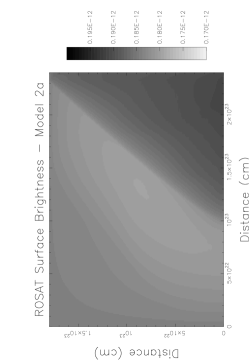
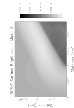
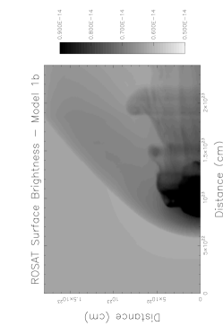
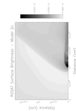
Figure 7: Synthetic ROSAT surface brightness profiles for the four simulations shown in Figs. 1 and2. Top left panel: Model 2a; top right panel: Model 3d (both ES mode). Bottom left panel: Model 1b; bottom right panel: Model 2c (both MR mode). The synthetic surface brightness images have been calculated in the $0.1-2.5\,\mbox{${\,\rm keV}$}$ waveband, with units of ${\,\rm erg~{}cm}^{-2}{\rm s}^{-1}{\rm arcmin}^{-2}$ . Note that emission from the cluster has been included. Careful attention should be paid to the scaling of these images, as some of them have a much larger dynamic range than others.

4 Observable Consequences

One of the main purposes of this paper is to investigate the expected observable properties of the theoretical simulations of the galaxy/ICM interaction, with an emphasis on the X-ray waveband. As most of the current data have been taken with the ROSAT satellite (the $0.1-2.5\,\mbox{${\,\rm keV}$}$ waveband) this is the spectral region we concentrate on, though future work will look at both the XMM and Chandra wavebands.

The hydrodynamic simulations (Figs. 1 and 2) provide values of $\rho$ and $T$ at all locations, and then it is straightforward to generate synthetic X-ray surface brightness maps for the simulations. The basic synthetic X-ray surface brightness maps for the four simulations in Figs. 1 and 2 are shown in Fig. 7. These images are for the $0.1-2.5\,\mbox{${\,\rm keV}$}$ waveband, and the background cluster emission (appropriate for the waveband and for the cluster surface brightness - Section 2.2) has been added. The cluster emission is often greater than the emission from the wake or bow-shock region and this has the effect of making the contrast between the tail or wake and background emission small. The effects of Galactic absorption are not included in Fig. 7 as they are likely to be of little consequence. It is necessary to carefully look at the scales in Fig. 7 to determine the visibility of the various structures. The images can either have a large (i.e. Model 1b) or small (the ES mode simulations) dynamic range, and the scaling has been adjusted appropriately. The important features to notice in Fig. 7 are as follows:

1. For the ES mode simulations the most prominent structures are the bow-shocks, with a small deficit of emission preceding the bow shock. This is due to the lower density region caused by the gravitational acceleration of material by the galaxy.

2. For the hotter cluster simulations (see Model 3d), the cluster background is very bright, and the contrast between bow-shock and background is small ($\sim 1$ per cent). This is more apparent in Fig. 8, where surface brightness slices are shown for all 4 simulations. This means that interaction effects will be more likely to be seen in cooler, less luminous clusters.

3. For the MR mode (Models 1b and 2c) there are three main features visible in the synthetic images. First, the bow-shock, second elongated emission from the tail region and third emission from the galaxy itself.

4. For Model 1b, the galaxy is very luminous, and in order to enhance the visibility of the tail and bow-shock region we do not show the full dynamic range (c.f. Fig. 8). There is a large accumulation of material at the galaxy centre. However, this emission, essentially analogous to a cluster cooling flow, will likely be strongly absorbed in a real galaxy.

5. For Model 2c, both the bow-shock and tail are visible, but the tail is less pronounced that for Model 1b.

6. For both Model 1b and Model 2c the emission from the tail does stand out substantially from the cluster background. However, the contrast for the bow-shock is less. This seems to be a general characteristic - the bow-shock is always less visible than any ram-pressure stripped tail.

7. For Model 1b the synthetic image shows considerable substructure on a scale of around $5-10{{}^{\prime\prime}}$. Such structures should be clearly visible with Chandra and XMM.

To further illustrate these points, in Fig. 8 surface brightness slices are shown. These slices have been generated by taking a slice of width $10^{22}$ cm along the $x$-axis. For the ES cases (Models 2a and 3d as examples) the increase in surface brightness is relatively small (a few per cent at most) and the surface brightness profile is relatively simple. For the MR mode case there are much greater increases in emission. Taking Model 1b as an example, the region associated with the galaxy is extremely bright, but the tail region also shows a substantial increase, with an excess brightness over the background of $\sim 10-30$ per cent. Even the case of Model 2c, which shows less in the way of enhanced emission at the position of the galaxy, has a tail for which the surface brightness is more than the $\sim 10$ per cent greater than the underlying cluster.

For both the MR mode simulations in Fig. 8, there is substantial substructure in the surface brightness in the tail region, with regions of enhanced emission associated with blobs of gas stripped from the galaxy. The bow-shock region in the MR mode cases extends further in front of the galaxy than for the ES mode cases.

For our simulations we have generated hardness ratio maps, with the hardness ratio defined as $(H-S)/(H+S)$, where $H$ is the hard-band ($0.5-2.5\,\mbox{${\,\rm keV}$}$) image and $S$ the soft-band image ($0.1-0.5\,\mbox{${\,\rm keV}$}$). The results in Table 3 show that for the MR mode the tail region is cooler than the ambient cluster, and consequently spatial hardness variations might be expected. However, because the temperature differences are usually small and the emission from the tail region is always small compared to the background cluster emission, this means that differences in the hardness ratio are always small.

Figure 8: Surface brightness slices for the four images shown in Fig. 7. The units are ${\,\rm erg~{}cm}^{-2}{\rm s}^{-1}{\rm arcmin}^{-2}$ . These slices in surface brightness are taken along the $x$-axis through the galaxy for a slice with a width of $10^{22}$ cm. The level of background cluster emission varies substantially from the cool to the hot cluster. Also note that the scale for Model 1b has been truncated to enhance the contrast in the tail region. The peak surface brightness for this model is $\sim 10^{-11}\mbox{${\,\rm erg~{}cm}^{-2}{\rm s}^{-1}{\rm arcmin}^{-2}$\,}$. Note the substructure in the tails of the MR mode simulations.

5 Discussion

In this paper we have presented some new simulations of the interaction between galaxies and the ICM in clusters. For the first time we have attempted to quantify the likely observational characteristics of structures resulting from such interactions, with some promising results. Galaxies which are capable of retaining some mass and have substantial tails are likely to have features that are observable. However, those that are completely ram-pressure stripped are unlikely to have observable features. The bow-shock is a more prominent feature in MR mode galaxies than in ES mode galaxies (Figs. 7 and 8).

The likely criterion for galaxies to show observable interaction effects in clusters are as follows:

1. Galaxies with younger stellar populations (and hence more substantial mass-loss) are more likely to show interaction effects at X-ray energies.

2. Galaxies in cooler clusters or group will be more likely to have observable stripped tails. Galaxies in rich clusters will be more likely to be completely stripped.

3. Galaxies in lower surface brightness clusters - in richer, brighter clusters the contrast between tail and background emission is smaller.

4. Galaxies at the periphery of rich clusters. Massive gas-rich galaxies infalling into rich clusters should show tails.

This means that bluer galaxies in nearby cooler clusters are the most likely place to look for such interaction effects. For rich clusters, such as Coma, most galaxies are likely to be completely stripped, except those at the periphery of the cluster, which may be in an environment where they can retain some mass. These simulations have also shown that while tails may be a feature of galaxies in clusters of all levels of richness the effects are more likely to be seen in the cooler clusters.

The potential rewards of being able to exploit the galaxy/ICM interactions are great (Merrifield 1998), however these simulations show the dynamics are complicated and the level of emission from the tail (for instance) will depend on parameters that may be difficult to determine (such as $\dot{M}_{rep}$). Consequently, it may take a substantial effort at modelling individual galaxies to fully determine the true velocity vector for that galaxy. The other, simple approach, to merely use the galaxies direction of motion on the plane of the sky (as revealed by a linear trailing structure), may also be able to yield interesting results.

The assumptions made here have been chosen to be simple and to be the most favourable. For example, we have assumed the galaxies to be spherical. In reality, the galaxies will be elliptical and the gas flow out of the galaxy will depend on the orientation of the galaxy with respect to its velocity vector through the ICM. For instance, it might be anticipated that mass might be lost more easily from the galaxy through the minor axis of the galaxy. We have also assumed that we are viewing the galaxy in the plane of the sky. If the galaxy is moving at a different angle then projection effects will play a role, foreshortening the tail and potentially making identification of galaxy/ICM features difficult. The effect of both of these assumptions will have to be explored with more sophisticated simulations. While certain orientations of an elliptical galaxy can be dealt with by 2-D simulations, the more general case of random galaxy orientation will require 3-D simulations

For several of the suspected examples of galaxy/ICM interaction (Section 1) all that can be discerned about the dynamic structures associated with the galaxy motion is an extension of the X-ray contours away from the cluster centre (usually interpreted as due to infall of the galaxy towards the cluster centre). Examples of this are NGC 4839 in the Coma cluster (Dow & White 1995) and NGC 1404 (Jones et al. 1997). It is notable that NGC 4839 is located towards the edge of the Coma cluster, where we might expect interactions effects to be more visible.

In the case of M86, in addition to an emission peak at the galaxy centre, there is also a second peak associated with the tail. These simulations and those of Balsara et al. (1994) suggest that stripping will often occur in discrete events, with blobs of material being removed. These blobs will result in enhancements in the tail region, and this is what may be occurring in M86.

NGC 4472 shows very complex emission, with some evidence of a bow-shock as well as a tail. This galaxy will clearly require more detailed work on it. Irwin & Sarazin (1996) suggest that some of the features may be related to the elliptical nature of the galaxy and its orientation with respect to its motion. This idea will clearly have to be tested with further simulations allowing for non-spherical galaxies.

In summary, we have new presented calculations of the galaxy/ICM interaction in clusters, with particular emphasis on investigating the likely observable consequences of such interactions. From these simulations it is clear that many galaxies should show observable effects of the galaxy/ICM interaction, the most prominent feature being linear tails, resulting from ram-pressure stripping. We have performed simulations for a wide range of cluster parameters, with the goal of trying to define the best parameter space to investigate. While massive galaxies, with young stellar populations, in cool nearby clusters such as Virgo or Fornax offer the best possibilities, the periphery of richer clusters also offers interesting possibilities. An important result is that it is not galaxies that are completely ram-pressure stripped that have the brightest tails, but rather those which are able to retain a substantial fraction (but not all) of the replenished material. In this situation, stripping occurs in discrete events and results in high density tails. Bow-shocks should also be visible in some galaxies, particularly in upcoming XMM and Chandra observations of nearby candidates. There are good prospects that, through a combination of modelling and observations with the new X-ray observatories, galaxy/ICM interactions offer a new window to investigating cluster dynamics.

References

- [1] Abadi M. G., Moore B., Bower R. G., 1999, MNRAS, (in press)
- [2] Balsara D., Livio M., O’Dea C., 1994, ApJ, 437, 83
-
[3]
Blondin J. M., Kallman T. R., Fryxell B. A., Taam R. E.,
1990, ApJ, 356, 591
- [4] David L. P., Jones C., Forman W., Daines S., 1994, ApJ, 428, 544
- [5] Dow K. L., White S. D. M., 1995, ApJ, 439, 113
- [6] Djorgovski S., Davis M., 1987, ApJ, 313, 59
- [7] Faber S. M., Gallagher J. S.,, 1976, ApJ, 204, 365
- [8] Gaetz T. J., Salpeter E. E., Shaviv G., 1987, ApJ, 316, 530
- [9] Gunn J. E., Gott J. R., 1972, ApJ, 176, 1
- [10] Hunt R., 1971, MNRAS, 154, 141
- [11] Irwin J. A., Sarazin C. L., 1996, ApJ, 471, 683
- [12] Jones C., Forman W., 1984, ApJ, 276, 38
- [13] Jones C., Stern C., Forman W., Breen J., David L., Tucker W., Franx M., 1997, ApJ, 482, 143
- [14] Loewenstein M., Mushotzky R. F., 1996, ApJ, 471, L83
- [15] Mamon G. A., 1987, ApJ, 321, 622
- [16] Mathews W. G., 1989, AJ, 97, 42
- [17] Matt G., Prio L., Antonelli L.A., Fink H.H., Meurs E.J.A., Perola G.C., 1994, A&A, 292, L13
- [18] Merrifield M. R., 1998, MNRAS, 294, 347
- [19] Mulchaey J. S., Davis D. S., Mushotzky R. F., Burstein D., 1996, ApJ, 456, 80
- [20] Nulsen P. E. J., 1982, MNRAS, 198, 1007
- [21] Ponman T. J., Bourner P. D. J., Ebeling H., Bohringer H., 1996, MNRAS, 283, 690
- [22] Ponman T. J., Cannon D. B., Navarro J., 1999, Nature, 397, 135
- [23] Portnoy D., Pistinner S., Shaviv G., 1993, ApJ, 86, 95
- [24] Rangarajan F. V. N., White D. A., Ebeling H., Fabian A. C., 1995, MNRAS, 277, 1047
- [25] Sakelliou I., Merrifield M. R., McHardy I. M., 1996, MNRAS, 283, 673
- [26] Schweizer F., 1982, ApJ, 252, 455
- [27] Shaviv G., Salpeter E. E., 1982, ApJ, 110, 300
- [28] Stevens I. R., Blondin J. M., Pollock A. M. T., 1992, ApJ, 386, 265
- [29] Takeda H., Nulsen P. E. J., Fabian A.C., 1984, MNRAS, 208, 261
- [30] Tully R. B., 1987, ApJ, 321, 280
- [31] Veilleux S., Bland-Hawthorn J., Cecil G., Tully R.B., Miller S.T., 1999, ApJ, (in press)
- [32] White D. A., Fabian A. C., Forman W., Jones C., Stern C., 1991, ApJ, 375, 35
- [33] White D. A., Fabian A. C., 1995, MNRAS, 273, 72
- [34] White D. A., Jones C., Forman W., 1997, MNRAS, 292, 419