The Extraordinarily Rapid Expansion of the X-ray Remnant of Kepler’s Supernova (SN1604)

Abstract

Four individual high resolution X-ray images from ROSAT and the Einstein Observatory have been used to measure the expansion rate of the remnant of Kepler’s supernova (SN 1604). Highly significant measurements of the expansion have been made for time baselines varying from 5.5 yrs to 17.5 yrs. All measurements are consistent with a current expansion rate averaged over the entire remnant of $0.239^{+0.015\,+0.017}_{-0.015\,-0.010}\,\%\,\rm yr^{-1}$, which, when combined with the known age of the remnant, determines the expansion parameter $m$, defined as $R\propto t^{m}$, to be $0.93^{+0.06\,+0.07}_{-0.06\,-0.04}$. The error bars on these results include both statistical (first pair of errors) and systematic (second pair) uncertainty. According to this result the X-ray remnant is expanding at a rate that is remarkably close to free expansion and nearly twice as fast as the mean expansion rate of the radio remnant. The expansion rates as a function of radius and azimuthal angle are also presented based on two ROSAT images that were registered to an accuracy better than $0\mskip 1.0mu^{\prime\prime}\mskip-7.0mu.\mskip 2.0mu5$. Significant radial and azimuthal variations that appear to arise from the motion of individual X-ray knots are seen. The high expansion rate of the X-ray remnant appears to be inconsistent with currently accepted dynamical models for the evolution of Kepler’s SNR.

1. Introduction

The remnant of Kepler’s supernova (SN) is the youngest of the historical supernova remnants (SNRs) with an accurate, well-established explosion date (A.D. 1604). Although long suggested to be the remnant of a Type I SN based on its light curve (see Doggett & Branch 1985), recently it has been proposed that it was the explosion of a massive star. Numerous studies of Kepler’s SNR, from the optical work of van den Bergh & Kamper (1977) to the X-ray studies of White & Long (1983) and Hughes & Helfand (1985), have concluded that SN 1604 exploded in a dense environment, a conclusion that is strongly at odds with the remnant’s large distance above the Galactic plane. The model introduced by Bandiera (1987) in which the progenitor was a rapidly-moving mass-losing star, provided a significant breakthrough in our understanding of the nature of Kepler’s SNR. This model was able to explain both the high ambient density and the strongly asymmetric appearance of the remnant in both the X-ray and radio bands. However, it also indicated that the dynamics of the remnant should be extremely complex with reflected and transmitted shocks propagating through the SN ejecta as well as pre-existing structures in the circumstellar medium (CSM) (Borkowski, Blondin, & Sarazin 1992). In light of this complexity it is clear that measurements of the dynamics of Kepler’s SNR using as many different methods as possible, are going to be an important ingredient in understanding the evolution of the remnant. In this article I present the first results on the current expansion rate of the X-ray remnant of Kepler’s supernova.

Previous expansion measurements of Kepler’s SNR have been done in both the optical and radio band. For reference the time-averaged expansion rate of Kepler’s SNR based on the full extent of the remnant in either the radio or X-ray band and its well-known age is $\sim$$0\mskip 1.0mu^{\prime\prime}\mskip-7.0mu.\mskip 2.0mu25$ yr^-1. The brighter optical knots in Kepler are expanding quite slowly, with an expansion timescale of $\sim$32,000 yr (Bandiera & van den Bergh 1991), a rate that is about two orders of magnitude slower than the time-averaged expansion of the remnant itself. Their slow motion and high nitrogen abundance (Dennefeld 1982; Blair, Long, & Vancura 1991) indicate a circumstellar origin for the dense radiative knots, an idea originally proposed by van den Bergh & Kamper (1977). The discovery of nonradiative, Balmer-dominated, optical filaments in Kepler’s SNR (Fesen et al. 1989) provided the opportunity to measure the shock velocity (albeit at a few specific locations in the remnant) from the width of the broad H$\alpha$ emission-line, which Blair et al. (1991) found to yield average shock velocities of 1550–2000 km s^-1.

Table 1Observations of Kepler’s SNR

Observatory	Start Date	Average MJD	Duration (s)
Einstein (E1)	1979 Sep 29	44146.62	$\phantom{0}5593.9$
Einstein (E2)	1981 Mar 22	44686.33	$12064.0$
ROSAT (R1)	1991 Sep 11	48511.17	$36143.2$
ROSAT (R2)	1997 Mar 10	50522.68	$67895.3$

Radio images of Kepler’s SNR from the VLA taken at two epochs (1981 and 1985) were used by Dickel et al. (1988) to determine the current expansion rate. Since the age of the remnant is known, it is possible to determine the expansion parameter, $m$, which is defined as $R\propto t^{m}$ (i.e., the remnant’s radius is assumed to evolve as a power-law with age). Dickel et al. (1988) found a best-fit value of $m=0.50$ averaged over the entire remnant, with a likely range including random and systematic uncertainties of $0.49<m<0.56$. Variations in the expansion rate with azimuthal angle were seen too. The expansion parameter of the radio remnant is higher than that expected from a SNR in the Sedov (1959) phase of evolution expanding into a uniform, isotropic interstellar medium ($R\propto t^{2/5}$). On the other hand, the observed value is lower than the expansion parameter expected for a Sedov-phase SNR expanding into a steady stellar wind ($\rho\sim r^{-2}$) density profile ($R\propto t^{2/3}$). However, neither of these models is strictly applicable, since Kepler’s SNR is believed to be in an earlier evolutionary phase than Sedov, where, after all, the ejecta are supposed to be dynamically unimportant.

The X-ray emission of Kepler’s SNR is dominated by emission lines from Si, S, Ar, Ca, and Fe (Becker et al. 1980; Kinugasa & Tsunemi 1994) with inferred abundances that are highly enriched compared to the solar values (Hughes & Helfand 1985). The conclusion that a significant fraction of the X-ray emission comes from shock-heated SN ejecta is compelling (Decourchelle et al. 1997). The X-ray–emitting material constitutes far more mass than that visible in the optical or radio band and so studies of the dynamics in the X-ray band are particularly important for understanding the evolution of the remnant. High angular resolution X-ray imaging is currently available only in the soft X-ray band (photon energies below $\sim$2 keV), where the flux from Kepler is overwhelming dominated by Fe L-shell ($n$p – 2s transitions) and Si XIII K$\alpha$ line emission.

X-ray expansion measurements of young SNRs are now possible for a couple of reasons. First, the ROSAT high resolution imager (HRI) operated for long enough that significant time baselines between individual ROSAT observations of a few remnants are available. Second, the HRIs on ROSAT and Einstein are similar enough that it is practical to take advantage of the considerably longer time baselines between pairs of observations taken by these different observatories. The Kepler radio expansion rates suggest an increase in the size of the X-ray remnant of $\sim$$0\mskip 1.0mu^{\prime\prime}\mskip-7.0mu.\mskip 2.0mu5$ over a 5 year time period, which is close to the limit of what is possible to detect with available HRI data. For Kepler’s SNR good data from both X-ray observatories are available and in particular deep first and second epoch observations separated by 5.5 yr were made by ROSAT. As I show below, agreement of the results determined from the various combinations of ROSAT and Einstein data provides a considerably higher level of confidence in the results than any individual pair of observations do.

2. Observations

2.1. Initial Data Reduction

Table 1 provides a log of all the high resolution Einstein and ROSAT imaging observations of Kepler’s SNR. The columns list the observatory, start date, the Modified Julian Day (MJD) corresponding to the average date of the observation, and the effective duration.

The remnant was observed twice by the Einstein high resolution imager (EHRI): first on 1979 Sep 29 and then later on 1981 Mar 22 for live-time corrected exposures of 5593.9 s and 12064.0 s, respectively. In the following I refer to these observations as E1 and E2. The background level in each observation was estimated separately and a value of $5.7\times 10^{-3}$ cts s^-1 arcmin^-2 was found to be consistent with both. There were roughly 8500 total detected events above background from Kepler’s SNR in observation E1 and 16,400 in E2 for rates of 1.51 s^-1 (E1) and 1.36 s^-1 (E2). The difference in rates is believed to be due to a reduction in the sensitivity of the EHRI during the course of the Einstein mission (Seward 1990).

Kepler’s SNR was first observed by the ROSAT HRI (RHRI) beginning on 1991 Sept 11 for a live-time corrected exposure of 36143.2 s and the observation was completed about a day later. I refer to this as R1 in the following. Due to the higher sensitivity and better calibration of the RHRI compared to the EHRI, plus the much deeper ROSAT exposures resulting in more than 10 times as many detected events, I have carried out a more detailed reduction of the ROSAT data. Throughout the entire data reduction process the pulse height range of the R1 data was restricted to include only channels 1 to 9. This reduced the background level significantly (by roughly 12%), while it hardly changed the number of X-ray events from the source (reduced by 1.2%). Aspect drift during the observation was a concern that was addressed in the following manner. A separate image was made from each of 15 time intervals (each typically 2000 s long) corresponding to individual orbits during the observation. Since there were no bright X-ray point sources in the field, the remnant itself was used to align the individual images using the IRAF task crosscor (in package stsdas.analysis.fourier). The initial registration of the individual maps from the standard analysis was fairly good: all of the individual maps were already aligned to within 1^′′ or better. The images from all the sub-intervals were registered to the nearest $0\mskip 1.0mu^{\prime\prime}\mskip-7.0mu.\mskip 2.0mu5$ pixel, shifted, and added.

The second epoch RHRI observation (R2 hereafter) began on 1997 Mar 10, ended on Mar 18 and included 67895.3 s of live-time corrected exposure. For this observation I used a range of pulse height channels from 1 to 6, which reduced the background level by 16% and the number of source X-ray events by 1.4% compared to the entire range of pulse height channels. Here I divided the data into 36 individual time intervals to check and then compensate for any aspect reconstruction errors. Most of the individual maps were already aligned to within better than 1^′′, but there were 3 separate intervals which produced offsets in declination of 2^′′–3^′′. Again the images were registered to the nearest $0\mskip 1.0mu^{\prime\prime}\mskip-7.0mu.\mskip 2.0mu5$ pixel, shifted, and added. For both epochs, this shift-and-add alignment technique produced images with a noticeably improved point response function.

Since the nominal RHRI background level integrated over the area of the SNR represents slightly more than 1% of the remnant’s count rate, I exerted some effort to estimate accurate values of the background level in the two pointings. This estimate is made difficult by the significant grain scattering halo from Kepler’s SNR (Mauche & Gorenstein 1986; Predehl & Schmitt 1995) and in fact careful inspection of the data reveals that the entire RHRI field of view contains some emission from the scattering halo. (Because of the higher background the scattering halo is much less prominent in the Einstein observations.) To estimate the RHRI background level I fitted a spatial power-law component plus a constant background level to the surface brightness profile over the $2^{\prime}\mskip-5.0mu.5$ to 15^′ radial range. The fitted power-law components were consistent between the two pointings (index of $-$1.5), although the background levels differed by some 40%, $3.2\times 10^{-3}$ cts s^-1 arcmin^-2 for the first pointing and $2.4\times 10^{-3}$ cts s^-1 arcmin^-2 for the second pointing. This difference is within the variation observed from field to field for the RHRI (David et al. 1998).

The two RHRI observations were separated in time by roughly a half-integer number of years, so the roll angles of the two pointings differ by nearly 180^∘. This means that spatial variations in the efficiency of the detector will not cancel out between the two pointings, so it was necessary to make an exposure map for each observation. The table of pointing directions as a function of time (supplied as part of the ROSAT standard processing) was binned into a map containing the fractional amount of time the telescope spent viewing differing positions on the sky during each observation. This produced a roughly rectangular region of nearly uniformly sampled sky, 4^′ long (in the direction of the wobble) and about 1^′ wide. The average roll angles of the pointings were determined: $-$356^∘ (R1) and $-$173^∘ (R2). A well-sampled image of the bright earth was used to account for the spatial variation of the quantum efficiency of the HRI, including the effects of an imperfect gapmap. The bright earth map was rotated about the optical axis and then convolved with the sky viewing map to produce the exposure map. Linear interpolation was used to sample the map onto different pixel grids as appropriate. Over the portion of the field containing the image of Kepler’s SNR the ratio of exposure between the first and second epochs varied between 0.975 and 1.02.

The exposure- and deadtime-corrected, background-subtracted RHRI count rates of Kepler’s SNR are $5.491\pm 0.012\,\rm s^{-1}$ and $5.433\pm 0.009\,\rm s^{-1}$ from the first and second epoch images, respectively, within a radius of 4^′. Because of the remnant’s significant interstellar grain scattering halo, care was taken to make the regions used for extracting the source counts as similar as possible between the two epochs. From the measured count rates it would therefore appear that the total X-ray flux of Kepler’s SNR has declined by $\sim$1% over the course of 5.5 yrs. This, however, does not account for any possible changes in the instrument’s effective area over the same period. Temporal variations in the effective area of the RHRI have been monitored over the course of the mission by regular observations of the SNR N132D in the Large Magellanic Cloud, which is not expected to be variable on short ($\sim$10 yr) timescales. The available data (David et al. 1998) do not show any obvious secular trend, although the scatter in the observed count rates is considerably larger (RMS scatter of $\sim$ $\pm 3$%) than the statistical uncertainty in the individual measurements themselves (typically $\pm 1$%). This indicates that some other effects may be influencing the RHRI’s overall effective area, perhaps on an observation-to-observation basis. I conclude, therefore, that Kepler’s SNR shows no significant evidence for a change in X-ray flux although changes at the level of a few percent are possible.

2.2. Registration

Five weak X-ray point sources appeared in both the R1 and R2 images between 4^′ and 12^′ off-axis. I used these sources to register the different ROSAT images to each other (including position shifts as well as a rotation) and to constrain any changes to the RHRI plate scale empirically. According to the ROSAT standard processing there are no SIMBAD sources within 20^′′ of the nominal positions of these sources. I have not pursued the determination of absolute positions or the identification of optical or radio counterparts, since this information is not necessary for image registration.

The positions of the five sources in both observations were determined by fits of the appropriate off-axis RHRI point response function (David et al. 1998) to the image data, using a likelihood function derived for Poisson-distributed data as the figure-of-merit function. Pixel positions as well as their statistical uncertainties were determined. The differences between the fitted positions in the two epochs were compared using $\chi^{2}$. A single positional offset is a good fit to the five point sources: the $\chi^{2}$ associated with this fit is 8.1 for 8 degrees of freedom. The best fit difference in the pixel positions between the two epochs are $5\mskip 1.0mu^{\prime\prime}\mskip-7.0mu.\mskip 2.0mu0\pm 0\mskip 1.0mu^{\prime\prime}\mskip-7.0mu.\mskip 2.0mu4$ (in right ascension) and $-7\mskip 1.0mu^{\prime\prime}\mskip-7.0mu.\mskip 2.0mu6\pm 0\mskip 1.0mu^{\prime\prime}\mskip-7.0mu.\mskip 2.0mu3$ (in declination). The sense of the difference is that the second epoch image is south and east of the first. Figure 1 plots the individual offsets and uncertainties from the five point sources. The filled dot symbol shows the best fit positional offset and the dashed curve is the 1 sigma error contour (at $\Delta\chi^{2}=2.30$ as appropriate for two interesting parameters). There is no evidence for a relative rotation between the two epochs. If a rotation about the optical axis is allowed in addition to the positional shifts, the best fit rotation angle is found to be $0^{\circ}\mskip-5.0mu.04$ and the $\chi^{2}$ reduces to 7.5, which is not a statistically significant reduction relative to the unrotated fits.

Figure 1.— Positional offsets and uncertainties for five X-ray point sources serendipitously located in the field of view of both the first and second epoch HRI data of Kepler’s SNR. The best fit position for no relative rotation between epochs is shown as the filled dot symbol, while the dashed contour shows the 1 sigma uncertainty on that position.

Figure 2.— ROSAT HRI image of Kepler’s SNR. The left panel shows the summed data from two observations with a total exposure of 104 ks. The data were adaptively smoothed to an approximate signal-to-noise ratio per pixel of 5. This grayscale image here uses a square-root scaling for the image display. The contour values are logarithmically spaced by multiplicative factors of 1.864 and start at a value of 0.0865 counts s^-1 arcmin^-2. The effective resolution of the map, including both the instrumental PSF and the average width of the smoothing kernel, is shown at the lower left. The right panel shows the difference between the two observations, which were separated in time by 5.5 yr. Before subtraction the separate images were registered to the nearest $0\mskip 1.0mu^{\prime\prime}\mskip-7.0mu.\mskip 2.0mu5$ pixel and scaled by their respective exposure times. The grayscale image on this part of the figure uses a linear scaling for the image display and values are displayed between $\pm$0.36 counts s^-1 arcmin^-2. Dark regions are places where the count rate has dropped between the first and second epoch images and the light colored regions are places where the rate has increased. The contours of total X-ray intensity, which are the same as on the left panel, are shown for reference.

These sources also provide a limit on any changes to the RHRI plate scale over the 5.5 years that separate the first and second epoch images. I find that decreasing the plate scale (i.e., the number of arcseconds per pixel) of the second epoch observation by $0.16\%\pm 0.10\%$ (1-sigma uncertainty) resulted in a slightly better fit ($\chi^{2}=5.3$) to the relative positions of the point sources in the field. Using the positions of X-ray sources associated with globular clusters in M31 F. Primini (1995, private communication) has shown that the plate scale in July 1990 was $0.4992\pm 0.0004$ ^′′/pixel, while in July 1994 it was $0.4993\pm 0.0002$ ^′′/pixel which represents an increase of $0.02\%\pm 0.09\%$ in the ROSAT HRI plate scale over the course of 4 years. My intent here is not to claim that there has been a significant change in the plate scale of the ROSAT HRI (indeed my result is significant at only about the 90% confidence level), but rather to show that even this weak limit is still about a factor of 10 less than the expansion I measure for Kepler’s SNR. Below I use Primini’s and my values for the change in the RHRI plate scale as one estimate for the systematic errors on the expansion measurement.

Table 2Global Mean Percentage Expansion of Kepler’s SNR

Datasets	Time Difference (yr)	Expansion (%)
R1–R2	$\phantom{0}5.51$	$1.39^{+0.12}_{-0.13}\,{}^{+0.07}_{-0.18}$
E2–R1	$10.47$	$2.21^{+0.25}_{-0.26}\,{}^{+0.18}_{-0.05}$
E1–R1	$11.95$	$2.88^{+0.44}_{-0.33}\,{}^{+0.34}_{-0.11}$
E2–R2	$15.98$	$3.68^{+0.22}_{-0.23}\,{}^{+0.11}_{-0.20}$
E1–R2	$17.46$	$4.49^{+0.30}_{-0.33}\,{}^{+0.16}_{-0.18}$

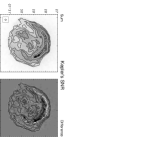
The five point sources allow accurate relative registration of the two ROSAT pointings. In figure 2, I show the sum of the two RHRI images as well as their difference after being registered and scaled by the ratio of live times. The latter shows a rim of positive emission around most of the periphery of the remnant with a region of negative flux further in, a clear signature of expansion.

3. Dynamics of the X-Ray Remnant

3.1. Global Mean Expansion Rate

The four Einstein and ROSAT observations give six different time baselines varying from $\sim$1.5 yrs to nearly 17.5 yrs over which it is possible to measure the expansion of Kepler’s supernova remnant. I use only the five longer baselines, since the shortest one, which corresponds to the two Einstein pointings, is also the one with the smallest number of detected events and thus is the least sensitive. Table 2 lists the five pairs of measurements used and the difference in time between the average date of each observation.

There are a number of complications associated with the comparison of these pairs of X-ray measurements. First, except for the two ROSAT pointings, there are no serendipitous point sources in the field that can be used for relative position registration. Second, small-scale spatial features in the remnant are neither bright enough nor distinct enough to be directly tracked from one observation to another. However Figure 2 clearly shows that there has been a significant change in the remnant during the time interval between the two ROSAT pointings. In the following I investigate whether these changes are consistent with the remnant undergoing expansion and determine numerical values for the rate of expansion.

The approach I take is to use the image from one of the observations as the “model” for the X-ray emission from the remnant, which is scaled in intensity, shifted in position, and expanded or contracted in spatial scale to match the image from another observation, referred to as the “data.” Note that for this part of the study there is no need to choose an expansion center. The model assumes that the expansion rate is uniform over the entire image of the remnant, both radially and azimuthally, and thus what I derive is a global mean expansion rate. Furthermore, this method is not sensitive to an overall translation or proper motion of the entire remnant. Any such translation is inextricably tied up with the relative registration of the various images (which in general is known to an accuracy of no better than 5^′′-10^′′ based on absolute positions from aspect reconstruction) and thus cannot be determined separately (for the moment I am ignoring the accurate registration between the two RHRI images, however see §3.2 below). Although the choice of which observation to use as the model or the data is arbitrary, in practice the deeper, later epoch observation is taken to be the model image. The figure-of-merit function for the model-data comparison is a maximum likelihood estimator derived for Poisson-distributed data. This is necessary since even for the second epoch ROSAT observation, which contains the largest number of detected X-rays, the most probable number of events in any 1^′′ square pixel over the central 2^′ image of Kepler’s SNR is 0, while the average number of events per pixel is $\sim$8. As is well known, this maximum likelihood figure-of-merit function does not provide an analytic goodness-of-fit criterion. However the function was implemented in such a way that differences in best-fit values were distributed like $\chi^{2}$, through the “likelihood ratio test” (see, for example, Kendall & Stuart 1979), which provided the basis for estimating statistical uncertainties. This technique of model fitting to two-dimensional imaging data and the software developed for it has been used in a number of situations; see Hughes & Birkinshaw (1998) for another example of its application and a more detailed description. The new software for this project was verified in a number of ways as explained below.

Some processing of the model image was unavoidable. In order to shift the image by a fractional number of pixels and expand or contract the spatial scale, some type of interpolation over the image had to be done. I used bilinear interpolation in right ascension and declination on a relatively smooth version of the model image. For the comparison of the two ROSAT pointings, the model image was adaptively smoothed. This was done by splitting the model data into a number of separate images according to surface brightness and smoothing each separate image with a different gaussian smoothing scale. The smoothing scales were chosen so that roughly the same number of counts on average were contained within a smoothing scale length in all the separate images. It is essential that the smoothing process not introduce any bias into the expansion measurement. This was verified by taking the same observation (R2) as both the data and model, carrying out this smoothing process on the model, and fitting for the relative position shift, the change in spatial scale, and the intensity change. The best fit relative position shift was $<$0.001^′′ and the best fit changes in spatial scale and intensity were both $<$0.01%, clearly indicating that the smoothing process has not introduced a bias into the fitted results.

I also rigged up a test to verify that this technique could accurately detect changes in the sizes of X-ray images (as opposed to a null test like above). The smoothed version of observation R2, which was constructed with $1^{\prime\prime}$ square pixels, served as the model. For the data the same observation, but blocked to $1\mskip 1.0mu^{\prime\prime}\mskip-7.0mu.\mskip 2.0mu5$ square pixels, was used. The software carries out the fits in terms of image pixels, so the two images clearly differ significantly in spatial scale and relative normalization. Nevertheless the software returned precise and accurate best-fit values for the spatial scale: $0.6664\pm 0.0002$ (expected value: 2/3) and relative normalization: $2.2473\pm 0.0014$ (expected value: 2.25) (1-sigma errors). This test and the others described in this section give confidence in the software and technique used for these expansion measurements.

For the comparison of the Einstein and ROSAT data, the most critical image processing step was to account for the differing on-axis point response functions (PRFs) of the two observatories. The Einstein PRF is somewhat broader and has a stronger scattering halo than the ROSAT one. In addition the Einstein PRF has some dependence on photon energy, while the ROSAT one is nearly achromatic. Parametric models of the PRFs for both instruments are available in the literature (Einstein: Henry & Henriksen 1986; ROSAT: David et al. 1998). As the first step, the Lucy-Richardson (Richardson 1972; Lucy 1974) algorithm was used to deconvolve the ROSAT PRF from the RHRI data. Beyond a certain point the results were relatively insensitive to the number of iterations of the algorithm; five or ten iterations were found to produce nearly identical results. The deconvolved image was then convolved with the Einstein PRF to produce a model image with a spatial resolution approximating that of the EHRI. This process produced a smooth enough model that no additional smoothing step was necessary. In general the fits of the model image were quite good (after accounting for the expansion of the remnant) and it is clear, at least qualitatively, that there was no gross mismatch in the PRFs. Toward the end of this section (see discussion of SNR N132D below) I describe how I verified quantitatively that the method just described does not bias the expansion measurement.

This now brings me to the discussion of the fits themselves. The first set of fits was done under the assumption that the remnant had not undergone any expansion. There were four parameters in these fits: relative position shift in right ascension and declination, ratio of intensity (or normalization), and background level. The data were fit over a circular portion of the HRI field with a radius of $2^{\prime}\mskip-5.0mu.5$ centered on the remnant. The results are summarized in the set of plots at the top of figure 3 which show the azimuthally-averaged surface brightness profiles for the five pairs of observations considered. Although the gross match between the data and model is good, plots of the residuals (second epoch minus first epoch) show an “S”-shaped pattern near the remnant’s edge that is a characteristic signature of expansion.

Figure 3.— Azimuthally-averaged radial X-ray surface brightness profiles of Kepler’s supernova remnant showing a pairwise comparison of observations taken at different times. The $\Sigma_{X}$ panels plot one observation as the “Data” (points with error bars) while another observation, after being shifted in position and scaled in intensity to match, is plotted as the “Model” (histogram). The various combinations of data and model are labelled at the top; note that the observation taken to be the “Data” is always the earlier one. The $\Delta\Sigma_{X}/\sigma_{\Sigma}$ panels show the residuals between the model and data. The set of panels at the top assume that the remnant has undergone no expansion over the period of time between observations (values as indicated). Note the characteristic pattern of residuals indicative of expansion of the remnant. The bottom set of panels assume that the remnant has expanded between observations and the best-fit expansion values for each pair of measurements are shown. In all cases these fits are a considerable improvement over the fits assuming no expansion. The ROSAT surface brightness data (first pair of panels on the left) have been divided by a factor of 3 in order to fit on the same scale at the Einstein data (remaining panels).

Figure 4.— Global mean percentage expansion of Kepler’s supernova remnant versus the time difference between imaging measurements. The five points come from using different pairs of measurements. The cross symbol, which indicates the shortest time difference, comes from comparing the two ROSAT pointings. The circles compare the ROSAT first epoch pointing with the Einstein second epoch (open symbol) and first epoch (filled symbol) observations. The squares show the expansion rate using the ROSAT second epoch pointing with the Einstein second epoch (open symbol) and first epoch (filled symbol) observation. The error bars show the statistical uncertainty, while the boxes that surround each data point give an estimate of the systematic uncertainty. The dotted curves show the expansion rate expected assuming expansion parameters of 0.8 (bottom curve), 0.9 (middle) and 1 (top). Remarkably, the X-ray remnant of Kepler’s SNR appears to be expanding at close to the free expansion rate.

In the next set of fits the mean expansion of the remnant expressed as a percentage was included as one additional free parameter. The resulting surface brightness profiles are shown in the plots at the bottom of figure 3. In all cases the quality of the fit improved significantly with the residuals now appearing quite flat. The reduction in the value of the likelihood function was 56 for the least significant case (E2 compared to R1) while it was over 800 for the most significant one (R1 compared to R2). According to the likelihood ratio test, as mentioned above, the distribution function for the change in the likelihood function in this case is given by a $\chi^{2}$ distribution with a single degree of freedom. Consequently the confidence levels associated with these reductions in the likelihood function are all off-scale (i.e., $\gg$ 3 sigma).

The best fit percentage expansion factors are plotted versus the time difference between observations in figure 4 and numerical values are presented in column 3 of table 2. The uncertainties quoted in the table consist of 1-sigma statistical uncertainties (the first pair of values) as well as systematic uncertainties (the second pair of values). The error bars in figure 4 show the statistical uncertainties, while the boxes drawn about each symbol indicate the level of systematic uncertainty. The five individual values are consistent at about the 1 sigma confidence level, assuming only statistical uncertainty, with an ensemble expansion rate of $\sim$0.24% yr^-1. However, these five individual values are not independent, so they cannot be combined directly. I can construct an ensemble average expansion value from independent pairs of observations in two different ways: E2-R2 and E1-R1, or E1-R2 and E2-R1. As a conservative estimate I take the maximum absolute value of the systematic uncertainty within each pair as the systematic uncertainty to associate with the ensemble value. These result in expansion rates of $0.239^{+0.015\,+0.017}_{-0.015\,-0.010}\,\%\,\rm yr^{-1}$ (E2-R2 and E1-R1) and $0.232^{+0.013\,+0.028}_{-0.013\,-0.013}\,\%\,\rm yr^{-1}$ (E1-R2 and E2-R1), where the first set of quoted errors comes from statistical uncertainty and the second set incorporates systematic effects. Because the former value has a smaller systematic uncertainty range (and since the two ensemble averages are fully consistent with each other at the 1-sigma level), I will consider the former value to represent the global mean expansion rate of Kepler’s SNR in the remainder of this article.

The quoted statistical errors are based on three sources of random noise: Poisson noise in the data image, Poisson noise in the model image, and the statistical uncertainty on the determination of the relative plate scale between pairs of observations. The total statistical error I quote is the root-sum-square combination of the three components. The first term was found in the usual manner by searching for values of the expansion that correspond to an increase in the figure-of-merit function of +1 above the best fit case (1 sigma confidence level). The second error term was assessed using a Monte Carlo approach which was carried out for each pair of data-model images. Simulated data were created from the adaptively smoothed ROSAT image that corresponds to the model using a Poisson random number generator, assuming the same exposure time as in the original image. For comparison with the Einstein data this simulated image was then run through the deconvolution and convolution steps discussed above that account for the differing instrumental PRFs. For comparison with the other ROSAT data the simulated image was adaptively smoothed. The best fit expansion value was determined using the processed, simulated image as the model and then the whole process was repeated until a total of 10 separate random realizations of the model were completed. The statistical error associated with the model was taken as the root-mean-square of the distribution of these best fit expansion values. In general for the ROSAT-Einstein comparison this term was a factor of 2 to 3 times smaller than the error from the Poisson noise in the data itself and thus does not cause a significant increase in the total error. However for the ROSAT-ROSAT comparison this term was comparable to the error from the noise in the data itself. The final source of statistical error was from the uncertainty in measuring any change in the plate scale between observations. For the ROSAT-ROSAT comparison the value of $\pm$0.10% uncertainty derived in §2.2 results in an identical uncertainty on the expansion of the remnant. This turns out to be the dominant source of random error for this pair of observations. I use a value of $\pm$0.07% for the error in determination of the relative plate scale between ROSAT and Einstein (David et al. 1998), which results in an error of the same size for the expansion. This error is small in comparison to the Poisson noise in the Einstein data.

Systematic uncertainties have the potential to bias the expansion measurement, so some effort was made to investigate them. For all pairs of data I studied the effects of varying the spatial region of the image over which the fits were done. The center of the circular fit region was shifted by 10^′′ in each of the four cardinal directions and the radius of the fit region was changed by $\pm$$0^{\prime}\mskip-5.0mu.5$. A new best-fit expansion value was obtained for each of these cases separately and the systematic uncertainty was taken to be the difference between the new value and the nominal best-fit value. The uncertainty due to the center shift was small, less than 0.06%, while that due to the size of the fit region ranged from 0 to a value as large as 0.2%. For the ROSAT-Einstein comparison two other effects were investigated: the number of iterations of the Lucy-Richardson deconvolution algorithm (between 5 and 10, which resulted in an uncertainty range of 0–0.07%) and changes in the modeled EHRI PRF. The functional form that describes the EHRI PRF depends on three parameters: two spatial scales and a relative normalization. Based on ground calibration data, the values of these parameters vary by roughly 10% as a function of photon energy over the $\sim$0.5–2 keV band and so this is the level of uncertainty I assume. Each of the three parameters was separately varied from its nominal value by $\pm$10% and new best-fit expansion values were obtained. The systematic uncertainties from this effect were all less than 0.07%. Finally for the ROSAT-ROSAT comparison, the change in plate scale was included as an uncertainty. According to the discussion in §2.2, the systematic errors resulting from possible changes in the RHRI plate scale are +0.02% and $-$0.16%, which are the dominant uncertainties for this pair of images. The several systematic errors are combined by direct summation to produce the values shown in table 2 and figure 4.

An additional possible source of systematic uncertainty arises from the difference in the effective area functions of Einstein and ROSAT. Because of the relatively high absorbing column density to Kepler’s SNR (estimates in the literature range from $\sim$$3\times 10^{21}$ cm^-2 to $\sim$$6\times 10^{21}$ cm^-2) the X-ray band below roughly 0.8 keV is largely absorbed away, so that the main difference in the effective area functions is Einstein’s greater sensitivity to X-rays with energies above 1.8 keV (see Vancura, Gorenstein, & Hughes 1995). Thus spatial variations in the X-ray spectral emissivity of the remnant could produce apparent differences in the relative flux seen by the EHRI compared to the RHRI. A strong radial gradient in the effective hardness of the remnant would be particularly pernicious since it would tend to appear predominantly as a radial increase or decrease in flux when the EHRI and RHRI data were compared that might masquerade as an expansion or contraction of the remnant. Although clearly a source of systematic uncertainty, it is unlikely that this effect is a significant source of bias in the results. The strongest arguments against this effect being important are (1) the good linear relationship found between the derived amount of expansion and the time baseline between observations (figure 4) and (2) the excellent agreement between the expansion rate for the ROSAT-ROSAT comparison (where there is no spectral band difference) and the ROSAT-Einstein comparison.

As an additional check on these overall results I carried out the same analysis for the SNR N132D in the Large Magellanic Cloud. Both the Einstein and ROSAT HRIs observed this remnant with the RHRI pointing being about a factor of 10 deeper than the EHRI one. The observations were separated by a span of roughly 11.6 yrs. N132D is a middle-aged remnant, about 4000 yrs old, roughly 12 pc in radius, with a shock velocity of approximately 800 km s^-1 (Hughes, Hayashi, & Koyama 1998). Over a span of 11.6 yrs, it should have expanded by a negligible amount, less than 0.1%. Following the same procedures and software as used for Kepler’s SNR I get an expansion rate for N132D of $-1.1^{+0.29}_{-0.25}\,{}^{+0.44}_{-0.55}$%, where again the first set of errors denote the statistical uncertainty and the second set denote the systematic uncertainty. The sign of the expansion indicates that the second epoch image of N132D (the RHRI one) is slightly smaller than the first, which is opposite to what was found for Kepler’s SNR, as well as somewhat implausible. The result may be due to the effect of spatial variations of the X-ray spectral emissivity from the remnant coupled with the different bandpasses of the Einstein and ROSAT HRIs. However, when the systematic errors are considered, the measured value of expansion for N132D is not significant, lying 2 sigma away from zero. This study is a more severe test of the null hypothesis for expansion because N132D is considerably smaller in angular size than Kepler’s SNR (45^′′ radius vs. 100^′′ radius), so that systematic effects due to the different point response functions are more significant. Nevertheless, the test confidently establishes that the expansion results on Kepler’s SNR are not an artifact of the analysis technique or procedures.

3.2. Expansion as a Function of Azimuth

Figure 5.— Variation of the best-fit spatial scale factor, intensity normalization, and reduced $\chi^{2}$ with azimuthal angle from a comparison of two ROSAT HRI observations of Kepler’s supernova remnant separated by approximately 5.5 yrs. Angles are measured east from north and the error bars are 1 sigma and are purely statistical. The dashed curve in the top panel is plotted at the reduced $\chi^{2}$ value corresponding to the 99% confidence level. The dashed curve in the middle panel corresponds to the ratio of detector live times.

The same software was used to determine the expansion rate as a function of azimuthal position around the remnant. The two RHRI observations were chosen for this part of the study since they were the most sensitive pair and subject to the least number of systematic errors. As before, the later epoch, adaptively-smoothed image served as the model which was scaled in intensity and spatial scale to match the earlier data. Comparison between the datasets was done for pie-shaped regions, centered on a fixed position (the expansion center, see below) with each region having an outer radius of $2^{\prime}\mskip-5.0mu.5$ and an angular extent of 20^∘. Separate fits were done for 36 angular regions centered on angles of 0^∘, 10^∘, 20^∘, etc. The sign convention used in this paper has angles increasing in a counterclockwise sense from north.

There were only two free parameters for each fit: the ratio of intensity normalizations (which would equal the ratio of detector live times if there were no changes in surface brightness) and the relative spatial scale between the epochs. The background was kept fixed at the nominal difference in background levels of $8\times 10^{-3}$ counts s^-1 arcmin^-2. Unlike before, no position shift was included, since the registration of the images is known, at least to $\sim$$0\mskip 1.0mu^{\prime\prime}\mskip-7.0mu.\mskip 2.0mu5$ or so. Instead the expansion is considered to be strictly in the radial direction about a position in the remnant, called the expansion center. I chose to take the center of the X-ray remnant at position 17:30:41 $-$21:29:23 (J2000) (determined by an eyeball fit of a circle to the outer X-ray surface brightness contours), as the location of the expansion center. In order to actually determine the expansion center it would be necessary to track individual X-ray emission features and determine the direction of their proper motion. Extrapolating several such tracks back to the center and noting where they intersect would then provide an estimate of the position of the expansion center. This is not yet possible to do in the X-ray band.

Figure 6.— The left side of the figure shows the X-ray emission from Kepler’s supernova remnant made by summing both ROSAT images and displayed using a square root intensity scale. The image shows the raw number of detected X-ray events per 1^′′ square pixel without background subtraction, smoothing, or exposure correction. The right side is a polar plot of the azimuthal expansion rates (solid curve) and 1 sigma statistical error range (dotted curves) from a comparison of the two ROSAT HRI observations. The dashed circles indicate the scale of this part of the figure in units of percentage expansion per year. Several azimuthal directions that correspond to features in the expansion rate plot are indicated on the grayscale image of the remnant (see text).

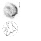
Figure 5 shows the results of these fits. The bottom panel shows the fitted relative spatial scale, expressed as a decimal fraction, required to make the second epoch data match the first epoch. (The scale factor is less than 1 because the second epoch image is larger than the first.) The 1-sigma error bars shown are rather small ($\pm$0.08%) in the bright northern part of the remnant but become much larger ($\pm$0.5%) in the faint southern part. They only include the statistical uncertainty in the data. The middle panel shows the ratio of fitted normalizations, which with one exception are all greater than the ratio of the detector live times (indicated on the plot as the dotted line). This indicates that the remnant has decreased in surface brightness between the two epochs and that the fainter regions toward the south have decreased more in brightness than the brighter northern regions. However the brightness decrease is offset by the increase in size of the remnant so that the total count rate from the remnant is nearly the same for the two epochs. Note that the (average) ratio of normalizations found here is consistent with the value determined from the global fits discussed above (§3.1). The top panel shows the $\chi^{2}$ per degree of freedom (for approximately 50 total degrees of freedom) associated with each best fit. For this calculation only, both the data and scaled model within each azimuthal sector were binned into a radial profile with 50 bins in radius. These surface brightness profiles were all visually inspected and no obvious systematic mismatch in the fits were apparent. However the reduced $\chi^{2}$ values shown in the figure scatter about a mean value of $\sim$1.5, indicating that the fits in general are formally unacceptable at about the 99% confidence level. It is likely therefore that other effects which have not been included in this analysis, such as non-radial motions, flux changes on small spatial scales, or radial variations in the expansion rate, are important for Kepler’s SNR. The first two topics are beyond the scope of this work, but the third topic is explored in the next section of the paper.

In order to check the relative registration of the two images once more, the fitted spatial scale factors, now expressed as a percentage expansion, were themselves fitted using $\chi^{2}$ to a function consisting of an azimuthally uniform expansion rate plus one that varied with angle as a sinusoid. The inclusion of the second term was highly statistically significant, resulting in a reduction in $\chi^{2}$ of at least 37 for the addition of two new free parameters. The best fit was obtained for a uniform expansion rate of 1.4% and a cosine function with an amplitude of 0.4% and phase angle of 207^∘. The effect of the sinusoid was to decrease the expansion rates in the north while increasing them in the south. The amplitude of the sinusoid could be caused by a relative position shift of as little as $0\mskip 1.0mu^{\prime\prime}\mskip-7.0mu.\mskip 2.0mu4$, which is of the same order as the computed error in the relative registration. Because of this, plus the excellent agreement of the uniform expansion rate determined here with the global mean value determined previously (§3.1), I have chosen to remove the fitted sinusoid from the azimuthal expansion rates. Note that the sinusoidal term sets a limit of $\sim$$0\mskip 1.0mu^{\prime\prime}\mskip-7.0mu.\mskip 2.0mu07\,\rm yr^{-1}$ on the overall proper motion of the X-ray remnant, corresponding to a limit on the transverse speed of $<$1660 $(D/5\,\rm kpc)\,km\,s^{-1}$. This should be interpreted only as a broad guide to the level of proper motion of the remnant excluded by the X-ray data since the amplitude of the sinusoid and thus the upper limit are sensitive to the somewhat arbitrary choice of expansion center made here.

The best fit model (uniform plus sinusoid) to the azimuthal expansion rates is formally not acceptable yielding $\chi^{2}=51$ for 15 degrees of freedom, indicating that there are significant azimuthal variations on smaller angular scales. This is obvious as well in figure 6 which shows the azimuthal expansion rates (corrected for the sinusoidal term) and the 1-sigma errors in a polar plot presentation. Next to it is a grayscale depiction of the X-ray image of the remnant. Some of the prominent azimuthal variations in expansion rate are correlated with emission features. The most rapidly expanding portion of the remnant at a position angle of 240^∘ contains a knot of emission about two-thirds of the way out from the center. This sector has an apparent expansion rate of $0.42\pm 0.04$% yr^-1. The two local minima in expansion rates at 50^∘ and 280^∘ are correlated with the edges of the bright northern portion of the shell. Other azimuthal variations do not appear to correlate with obvious emission features. These include the position of the peak expansion rate ($0.33\pm 0.02$% yr^-1) in the north at 350^∘ and the overall minimum in expansion rate ($0.10\pm 0.06$% yr^-1) at 150^∘. The pattern of azimuthal variation in expansion rates shown in figure 6 appears to be robust against modest changes in the position of the expansion center, as long as the sinusoidal term is fitted and removed. A second set of fits made with the expansion center displaced by about $2\mskip 1.0mu^{\prime\prime}\mskip-7.0mu.\mskip 2.0mu5$ gave results that agreed within the 1-sigma statistical errors with the previous fits. Finally, I point out that the overall scale of these azimuthal expansion results is additionally uncertain by roughly ${}^{+0.02}_{-0.05}$% yr^-1 due to systematic errors of which the plate scale uncertainty is the dominant one.

3.3. Expansion as a Function of Radius

Figure 7.— Radial X-ray surface brightness profile of Kepler’s supernova remnant from the ROSAT HRI (top panel) and the ratio of fitted normalizations (middle panel) and expansion rate as a function of radius (bottom panel) from a comparison of the two ROSAT HRI observations. The dashed line in the middle panel corresponds to the ratio of detector live times. The radial bins for the expansion measurements are not equally spaced in radius because the bin sizes were chosen to contain roughly equal numbers of detected X-ray events in each bin.

How the expansion rate of Kepler’s SNR varies with radius is also of interest. The procedure used here was the same as the one used to determine the azimuthal expansion rates with the exception that, instead of pie-shaped azimuthal regions, a number of disjoint (non-overlapping) annular regions centered on the position of the expansion center defined the separate regions over which individual fits were done. The annuli were not uniformly spaced in radius, but rather their various sizes were chosen so that each region contained roughly 20,000 X-ray events. The annular widths varied from a minimum of $4^{\prime\prime}$ right at the bright limb of Kepler’s SNR to a maximum of $\sim$40^′′ for the first radial bin in the fainter interior. It is not surprising that the radial expansion rates are sensitive to the relative registration of the two ROSAT images. For the results quoted here I used the best-fit registration from the previous azimuthal expansion study (i.e., corresponding to the one with no significant sinusoidal term). The expansion rates are shown in Figure 7 (bottom panel), along with, for reference, the X-ray surface brightness profile (top panel) and the ratios of fitted normalizations (middle).

The average of the radial rates plotted in fig. 7 weighted by their respective uncertainties yields a mean expansion rate of $\sim$0.23% yr^-1, which is entirely consistent with the global mean expansion rates determined previously (in both §3.1 and §3.2). Near the bright rim of the SNR, where the sensitivity to an expansion signal should be greatest, the radial expansion rates are in the range 0.17–0.28% yr^-1, with some indication that the rates are slightly higher on the inner edge of the rim, compared to the outer edge. Over some parts of the remnant interior the rates are remarkably high, a result of the apparent motion of the X-ray emitting blobs in this area. In particular the high rates for the second and third radial bin shown in fig. 7 are due to the rapidly moving knot at position angle 240^∘ pointed out earlier (in §3.2, also see fig. 6) that straddles both annular regions. The rates in the interior are also most sensitive to the choice of expansion center and the implicit assumption of purely radial motion. For example, if the expansion center is displaced by the same $2\mskip 1.0mu^{\prime\prime}\mskip-7.0mu.\mskip 2.0mu5$ shift used previously, the largest change in fitted rates occurs for the second radial bin which drops by 2.7 standard deviations, while the other points, particularly those near the bright rim, change much less.

The ratio of normalizations follows a very clear pattern. The results plotted in fig. 7, taken at face value, indicate that most of the remnant has decreased in X-ray surface brightness by about 4% over the time interval between RHRI observations. The outer edge of the remnant shell, however, has remained at constant brightness or has even increased slightly. These changes at the edge are statistically significant and are in addition to any changes in brightness caused by the remnant’s expansion. Note that the increase in overall surface area of the remnant, due to its expansion, compensates for most of the decrease in surface brightness so that the total count rate decreases by only about 1% between the two epochs, as mentioned earlier. Although the overall uncertainty on the temporal variation of the RHRI efficiency is of order a few percent (§2.1), it seems highly unlikely that the dramatic spatial variation in brightness seen here could be a result of instrumental changes.

4. Discussion

The extensive analysis described above is intended to convince the reader that a robust measurement of the expansion rate of the X-ray remnant of Kepler’s SN has been made. This confidence is based on deriving consistent values for the global mean expansion rate from fits

• over the entire X-ray image of the remnant for five different time baselines using high resolution images from both ROSAT and Einstein;

• as a function of azimuthal angle after correction for a relative registration error ($<$1^′′) between the two ROSAT observations; and

• as a function of radius for optimal relative position registration between the two ROSAT observations.

As indicated, the latter two methods use only the two ROSAT observations since they are the most sensitive and least susceptable to systematic errors. These different techniques all produce rates that are fully consistent with a value of $0.239^{+0.015\,+0.017}_{-0.015\,-0.010}\,\%\,\rm yr^{-1}$, which accounts for both statistical and systematic uncertainties. This result can also be expressed as an expansion time scale: $418^{+28\,+19}_{-24\,-27}\,\rm yr$. Kepler’s SNR is the remnant of a historical SN and so the age is known: it was 393 yr old in 1997. Comparison of the current expansion time scale to the age of the remnant reveals the extraordinary nature of these results. The X-ray remnant has appeared to undergone little or no deceleration since exploding as a supernova in 1604. Specifically, the expansion parameter, is measured to be $m=0.93^{+0.06\,+0.07}_{-0.06\,-0.04}$. In the following this result is examined in the context of other observational results as well as theoretical studies of the dynamics of Kepler’s SNR.

Optical knots are expanding quite slowly in Kepler’s SNR. Bandiera & van den Bergh (1991) determine an expansion time scale of 32,000 $\pm$ 12,000 yrs from the measured proper motions of some 50 knots of optical nebulosity, most of which are located toward the northwestern portion of the remnant. This corresponds to an expansion rate of $\sim$0.31 % century^-1, which is nearly two orders of magnitude smaller than the X-ray expansion rate. There is also a translation of the expansion center of the optical knots toward the northwest at a rate of $0\mskip 1.0mu^{\prime\prime}\mskip-7.0mu.\mskip 2.0mu8$ century^-1. The optical knots are believed to be circumstellar in origin, so their expansion would therefore largely arise from the motion of the original wind of the putative massive-star progenitor, plus some momentum imparted to them by the SN shock as well. The proper motion of the optical remnant itself, which is directed away from the Galactic plane, is strong evidence that the progenitor was a high velocity ($\sim$280 km s^-1) star that left the Galactic plane some $4\times 10^{6}$ yr ago, as originally proposed by Bandiera (1987). It is interesting to note that Bandiera & van den Bergh (1991) also find a number of optical knots (most of which lie near the edge of the shell) that appear to have brightened quite rapidly, with turn-on times of only a few years. Estimating these knots to be roughly 1^′′ in angular size and making the arguable assumption that the SN blast wave must be moving fast enough to fully engulf a cloud during its period of brightening, would suggest a shock speed on the order of $0\mskip 1.0mu^{\prime\prime}\mskip-7.0mu.\mskip 2.0mu2$ yr^-1. According to the X-ray image, the shock front is located at a radius of $\sim$100^′′, so this estimate of the shock speed is broadly consistent with the high X-ray expansion rates. Clearly this is not intended to be a precise estimate, but does indicate a plausible level of agreement.

The X-ray expansion rates of Kepler’s SNR are also much higher than the measurements in the radio band. Dickel et al. (1988) present a study of the expansion of Kepler’s SNR based on VLA radio data from two epochs separated by a time interval of about 4 yr. They find a mean expansion parameter for the entire radio remnant of $m=0.50$, as well as azimuthal variations that range from $m=0.35$ on the bright northern rim to $m=0.65$ on the eastern edge. These results are in considerable disagreement with the X-ray results, both in terms of the mean expansion rate and its variation with azimuth. However, Kepler is not the first remnant to show this dicrepancy: both Tycho’s SNR and Cas A are expanding more rapidly in the X-ray band than in the radio. The expansion parameter for Tycho’s SNR is $m=0.72\pm 0.10$ in the X-ray band (Hughes 1997) and $m\sim 0.47$ in the radio band (Strom, Goss, & Shaver 1982). Cas A has global expansion parameters of $m=0.73$ (X-ray) and $m=0.35$ (radio) (Koralesky et al. 1998, Vink et al. 1998). For Cas A there is also an indication that the size of the X-ray remnant is smaller than the radio remnant, although the size difference has been decreasing with time as the X-ray remnant catches up to the radio. A similar study comparing the sizes of the X-ray and radio images of Kepler’s SNR is beyond the scope of this paper but will be pursued in future work.

Chevalier (1982) has derived similarity solutions for the evolution of young SNRs that can be used to put the Kepler expansion results in some context. For ejecta with power-law density profiles characterized by index $n$ expanding into a circumstellar medium (CSM) with index $s$, the expansion of the remnant is given by $R\propto t^{(n-3)/(n-s)}$. For a stellar wind profile ($s=2$), the measured mean X-ray expansion rate for Kepler would suggest that the ejecta have a steep density distribution, $n\hbox{\raise 1.50696pt\hbox to0.0pt{$>$\hss}\lower 2.58334pt\hbox{$\sim$}\ }11$, similar to the atmosphere of a red supergiant. (A uniform density CSM, $s=0$ would require a considerably steeper density distribution for the ejecta profile to explain the mean X-ray expansion rate.) In order to explain the azimuthal X-ray brightness variations requires a difference in density from the northwest to the southeast (all other things being equal) of at least a factor of 3. In the Chevalier model the radius depends on the density of the stellar wind as $R\propto(1/q)^{1/(n-s)}$, so that if the density varies by a factor of 3, the radius should vary by a factor of $3^{-1/(n-s)}$. For $n>11$, then the remnant’s radius will vary by a factor between 0.89 and 1, and in other words, should appear quite round, as in fact Kepler’s SNR does.

The long-standing problem with this simple model has been in understanding the origin of the stellar wind’s strong azimuthal asymmetry. Bandiera (1987) realized that the interaction between the ambient interstellar medium (ISM) and the stellar wind from the rapidly-moving progenitor of Kepler’s SN would naturally produce an asymmetric CSM. This would consist of a dense bow-shock shell ahead of the star and an $r^{-2}$ stellar wind profile elsewhere, i.e., both within the shell and in the direction away from the star’s motion. The asymmetry of the observed remnant today reflects the interaction of the SN blast wave with the asymmetric CSM established by this process. Borkowski et al. (1992) examined this scenario in some detail and concluded that “the bow-shock model of Bandiera (1987) is currently the only model which accounts for most of the properties of this remnant.” The slow expansion of the radio remnant as a whole ($m\sim 0.50$) and in particular the very small expansion rate toward the northwest were considered strong evidence in support of the bow-shock shell model. However, this model should be re-evaluated in light of the much higher X-ray expansion results presented here. Furthermore it now appears to be the case for Kepler, as was found earlier for both Cas A and Tycho, that distinctly different magnetohydrodynamical structures are giving rise to the different radio and X-ray emissions.

5. Summary

In this article I have presented the first measurement of the expansion of Kepler’s SNR in the X-ray band. The remnant is expanding at a current rate averaged over the remnant of $0.239^{+0.015\,+0.017}_{-0.015\,-0.010}\,\%\,\rm yr^{-1}$, which is two orders of magnitude faster than the expansion of the optical knots and roughly twice as fast as the expansion of the radio remnant. Kepler is the remnant of an historical SN so the current rate can be compared to the time-averaged rate to indicate how much deceleration has occurred. Remarkably, the current and time-averaged rates are nearly equal implying that the remnant has hardly decelerated and is close to expanding freely. The expansion parameter of Kepler’s SNR is $m=0.93^{+0.06\,+0.07}_{-0.06\,-0.04}$, including both statistical and systematic uncertainty (the first and second set of errors, respectively).

There is significant variation of the expansion rate as a function of position in the SNR, although much of it does not appear to be correlated with obvious emission features. Of particular note is the finding that the faint, southeastern part of the remnant is expanding at roughly the same rate as the bright, northwestern part. The most rapidly moving feature in Kepler’s SNR is a knot of X-ray emission about two-thirds of the way out from the center in the southwestern quadrant, which has an expansion timescale of $\sim$250 yr, only a fraction of the remnant’s age. It is not clear what the origin of this motion is.

One might be tempted to use the X-ray expansion rate measured here and the shock velocity (1550–2000 km s^-1) determined from the properties of the H$\alpha$ emission (Blair et al. 1991) to estimate a distance to Kepler’s SNR. I resist this temptation, since it relies on a number of assumptions that are unlikely to be correct. Moreover, within the next year it will become possible, using Chandra, XMM, or Astro-E, to measure the Doppler shifts from bright X-ray emission lines of individual knots seen in projection near the center of the remnant. Combined with the X-ray expansion rate, this will provide a direct and independent measurement of the distance to Kepler’s SNR. To be strictly correct one will need to carry out the angular expansion measurement in the same emission line as the Doppler velocity mapping is done since chemical stratification of homologously-expanding ejecta would produce different expansion rates for different species.

The current best model for the evolution of Kepler’s SNR was developed to explain two important observations: the proper motion of the progenitor star and the high density of the ambient environment. This model has been shown to be consistent with a number of other observations as well, including the present slow expansion rate of the radio remnant. At first glance therefore it would appear that the extraordinarily rapid expansion rate of the X-ray remnant found here should be grossly inconsistent with these favored dynamical models. Future work should focus on this by identifying the magnetohydrodynamical structures, e.g., reverse shock, blast wave, reflected or transmitted shock, etc., that correspond to the X-ray and radio emission by modeling their dynamical and radiative processes.

Kepler is now the third young X-ray SNR to have its expansion rate measured; Cas A and Tycho are the others. In each of these three cases the same general effect is seen. The radio remnant and the X-ray remnant are of the same size, so the time-averaged expansion rates are quite similar. However the current expansion rate of the X-ray remnant is significantly larger than the current expansion rate of the radio remnant, clearly indicating that the structures in the remnant giving rise to the X-ray emission have been decelerated considerably less than the radio-emitting structures. Although perplexing, these differences in dynamical evolution are basic enough that they surely contain the seeds of some fundamental new insights into the nature and evolution of young supernova remnants.

References

- (1) Bandiera, R. 1987, ApJ, 319, 885
- (2) Bandiera, R., & van den Bergh, S. 1987, ApJ, 374, 186
- (3) Becker, R. H., Boldt, E. A., Holt, S. S., Serlemitsos, P. J., & White, N. E. 1980, ApJ, 237, L77
- (4) Blair, W. P., Long, K. S., Vancura, O. 1991, ApJ, 366, 484
- (5) Borkowski, K. J., Blondin, J. M., & Sarazin, C. L. 1992, ApJ, 400, 222
- (6) Chevalier, R. A. 1982, ApJ, 258, 790
- (7) David, L. P., Harnden, F. R., Kearns, K. E., Zombeck, M. V., Harris, D. E., Prestwich, A., Primini, F. A., Silverman, J. D., & Snowden, S. L. 1998, The ROSAT High Resolution Imager (HRI) Calibration Report.
- (8) Decourchelle, A., Kinugasa, K., Tsunemi, H., & Ballet, J. 1997, in the Proceedings of the International Conference on X-Ray Astronomy – ASCA 3rd Anniversary – X-Ray Imaging and Spectroscopy of Cosmic Hot Plasmas, (Universal Academy Press: Tokyo), eds. F. Makino & K. Mitsuda, 367.
- (9) Dennefeld, M. 1982, å, 112, 215
- (10) Dickel, J. R. Sault, R., Arendt, R. G., Korista, K. T., & Matsui, Y. 1988, ApJ, 330, 254
- (11) Doggett, J. B., & Branch, D. 1985, AJ, 90, 2303
- (12) Fesen, R. A., Becker, R. H., Blair, W. P., & Long, K. S. 1989, ApJ, 338, L13
- (13) Henry, J. P., & Henriksen, M. J. 1986, ApJ, 301, 689
- (14) Hughes, J. P. 1997, in the Proceedings of the International Conference on X-Ray Astronomy – ASCA 3rd Anniversary – X-Ray Imaging and Spectroscopy of Cosmic Hot Plasmas, (Universal Academy Press: Tokyo), eds. F. Makino and K. Mitsuda, 359
- (15) Hughes, J. P., & Birkinshaw, M. 1998, ApJ, 501, 1
- (16) Hughes, J. P., Hayashi, I., & Koyama, K. 1998, ApJ, 505, 732
- (17) Hughes, J. P., & Helfand, D. J. 1985, ApJ, 291, 544
- (18) Kendall, M., & Stuart, A. 1979, The Advanced Theory of Statistics, Volume 2 (New York: Macmillan), 246ff
- (19) Kinugasa, K., & Tsunemi, H. 1994 the Proceedings of the International Conference on X-Ray Astronomy – New Horizon of X-Ray Astronomy, (Universal Academy Press: Tokyo), eds. F. Makino & T. Ohashi, 469
- (20) Koralesky, B., Rudnick, L., Gotthelf, E. V., & Keohane, J. W. 1998, ApJ, 505, L27
- (21) Lucy, L. B. 1974, AJ, 79, 745
- (22) van den Bergh, S., & Kamper, K. W. 1977, ApJ, 218, 617
- (23) Mauche, C. W., & Gorenstein, P. 1986, ApJ, 302, 371
- (24) Predehl, P., & Schmitt, J. H. M. M. 1995, A&A, 293, 889
- (25) Richardson, W. H.. 1972, J. Opt. Soc. Am., 62, 55
- (26) Sedov, L. I. 1959, Similarity and Dimensional Methods in Mechanics (New York: Academic)
- (27) Seward F. D., 1990, ApJS, 73, 781
- (28) Strom, R. G., Goss, W. M., & Shaver, P. A. 1982, MNRAS, 200, 473
- (29) Vancura, O., Gorenstein, P., & Hughes, J. P. 1995, ApJ, 441, 680
- (30) Vink, J., Bloemen, H., Kaastra, J. S., & Bleeker, J. A. M. 1998, A&A, 339, 201
- (31) White, R. L., & Long, K. S. 1983, ApJ, 264, 196