Planetary Microlensing:
Present Status and Long-term Goals

Planetary Microlensing: Present Status and Long-term Goals

*

1 Introduction

Massive gravitational microlensing programs were begun about a decade ago as a means to search for compact baryonic dark matter in the Galaxy [2], but before the first events were detected [3, 4, 5] the technique was also proposed as a means of detecting extra-solar planets in our Galaxy [6].

Figure 1: Present microlensing planet detection programs are sensitive to planets similar to the one on the left; theoretical and observational capabilities must be increased by an order-of-magnitude before the long-term goal of reliably detecting planets similar to the one the right can be achieved.

Current microlensing planet searches, which have been underway for four years, are sensitive to jovian-mass planets orbiting a few to several AU from their parent Galactic stars. Within two years, sufficient data should be in hand to characterize or meaningfully constrain the frequency of massive planets in this range of parameter space, nicely complementing information about planets at smaller orbital radii now being provided by radial velocity searches. In principle, the technique could be pushed to smaller planetary masses, but only if a larger number of faint microlensed sources can be monitored with higher precision and temporal sampling. The VST on Paranal, with spectroscopic follow-up with the VLT, may be the ideal instrument for such an ambitious program.

2 Point lenses

As light rays from a distant background source S pass a distance $\xi$ from a gravitational point lens L of mass $M$, they are bent by an angle $\alpha={4\,G\,M}/{c^{2}\,\xi}$. Simple geometric arguments reveal that the two resulting images have an angular separation on the sky $\Delta\theta_{I}=\sqrt{{\theta_{\rm S}}^{2}+4\,{\theta_{\rm E}}^{2}}$, where ${\theta_{\rm S}}$ is the angular distance between the lens and the observer-source sight line and ${\theta_{\rm E}}$ is the angular Einstein ring radius, a characteristic size for the lensing geometry defined by

$${\theta_{\rm E}}\equiv\sqrt{\frac{4GM{D_{\rm LS}}}{c^{2}\,{D_{\rm OL}}\,{D_{\rm OS}}}}~{}~{}~{}.$$ (1)

Here ${D_{\rm OL}}$, ${D_{\rm OS}}$, ${D_{\rm LS}}$ are the observer-lens, observer-source, and lens-source distances, respectively (Fig. 2).

Figure 2: Point-lens microlensing geometry as seen from the side (left) and projected onto the sky (right). The images I₁ and I₂ straddle the source position on the sky.

Since the specific intensity of each ray remains unchanged, the magnification of the images is just the ratio of the image area to the source area, which can be found by evaluating at the each image position the determinant of the Jacobian mapping $J$ describing the lensing coordinate transformation:

$${\rm Magnification~{}Image~{}}_{i}=\left.\frac{1}{\hbox{ \vrule height=8.00003pt,depth=3.99994pt,width=0.6pt}\,\,det\,J\hbox{ \vrule height=8.00003pt,depth=3.99994pt,width=0.6pt}\,}\right|_{\,{\theta_{\rm I}}=\theta_{i}}=\left|\frac{\partial\,{{\theta_{\rm S}}}}{\partial\,{{\theta_{\rm I}}}}\right|^{-1}_{\,{\theta_{\rm I}}=\theta_{i}}~{}~{}.$$ (2)

The largest magnifications occur when the determinant is near zero. For a point lens this occurs when ${\theta_{\rm S}}\approx 0$ and the source lies almost directly behind the lens; the images then lie close to the Einstein ring ${\theta_{\rm E}}$. For lenses with stellar masses and distances typical for stars within the Milky Way, ${\theta_{\rm E}}\sim 1\,$mas, so that whenever the images are significantly magnified, they are too close together to be resolved by traditional imaging. Only the combined magnification $A$ of both images can be measured. For a point-lens, Eq. 2 can be used to show that $A=(u^{2}+2)/(u\sqrt{u^{2}+4})$, where $u\equiv{\theta_{\rm S}}/{\theta_{\rm E}}$ is the instantaneous source-lens separation in units of the angular Einstein radius.

Figure 3: Sample source trajectories (left) and the resulting light curves (right).

Because the source, lens, and observer are in relative motion, $u$ is a function of time. When $u$ is at its minimum, the observed light curve of the microlensing event undergoes its maximum magnification. Microlensing events for which the source has a small minimum impact parameter $u_{\rm MIN}$ will have the largest peak amplifications (Fig. 3). The characteristic time $t_{\rm E}\equiv{\theta_{\rm E}}{D_{\rm OL}}/v_{\perp}$ is the time taken by the lens, moving at speed $v_{\perp}$ across the sight line to the source, to travel one Einstein radius, and is a several days to months for most Galactic microlensing events.

3 Binary Lenses

Point lens light curves are symmetric because they are one-dimensional cuts through two-dimensional circularly-symmetric magnification patterns on the sky. Double lenses can generate more complicated light curves because this symmetry is broken. In particular, the loci of points in the source plane for which $\hbox{ \vrule height=8.00003pt,depth=3.99994pt,width=0.6pt}\,\,det\,J\hbox{ \vrule height=8.00003pt,depth=3.99994pt,width=0.6pt}\,=0$ have quite complicated structure (Fig. 4).

Figure 4: Single lens magnification map (left) and a binary lens fractional deviation map (right). The binary components (heavy dots) are separated by 1 ${\theta_{\rm E}}$ and have a total mass equal to the single lens. Regions where the binary magnification is depressed or increased by 1% and 5% relative to that of the single lens are marked by light and bolder contours, respectively. The very bold contour is the caustic.

These loci — called caustics — mark positions at which point sources would experience infinite image magnification. The observed flux remains finite as a caustic crosses a real source; integration over the source size $\theta_{*}$ is required to compute the observed total magnification. Sources passing near binary-lens caustics will exhibit light curves that deviate strongly from those of single lenses. The smaller the source and the closer the caustic approach, the larger the deviation will be. Unlike single lens curves, the shape of a binary light curve depends on the angle of the source trajectory through the magnification pattern.

Any static, unblended binary light curve is described by eight parameters: four quantities relevant to single lenses ($u_{\rm MIN}$, $t_{\rm E}$, time at peak $t_{0}$, and baseline flux $F_{0}$) and four additional parameters, namely, the binary mass ratio $q\equiv m_{1}/m_{2}$, the instantaneous angular separation $b$ of the components in units of ${\theta_{\rm E}}$, the ratio $\rho_{*}\equiv\theta_{*}/{\theta_{\rm E}}$ of source radius to Einstein radius, and the angle $\phi$ between the source trajectory and the binary axis.

4 Planetary Microlensing

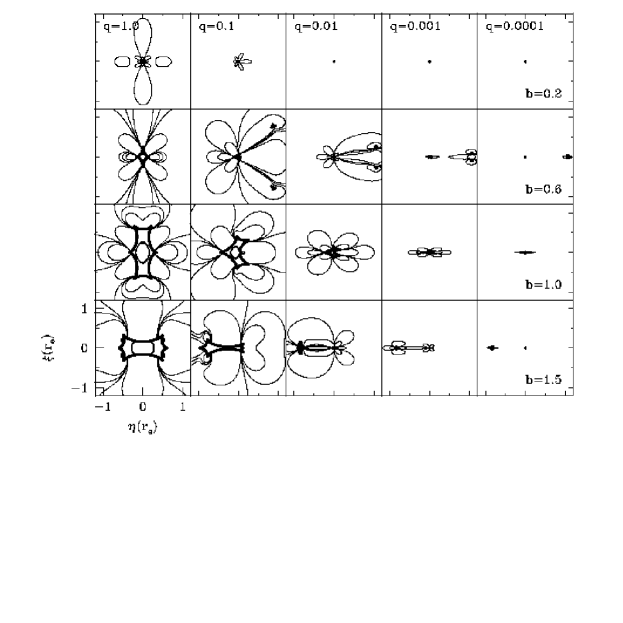
A lens orbited by one or more planets is a multiple lens and thus may have a magnification pattern that differs measurably from that of a single lens. Measuring and characterizing light curve deviations induced by planetary lensing companions is the goal of microlensing planet detection programs. The number, size and relative positions of the caustics depend on the mass ratio $q$ and separation $b$ of the double lens (Fig. 5).

Figure 5: Fractional deviation patterns for binary lenses with different mass ratios $q$ and separations $b$. Contours are the same as in Fig. 4; heavy lines are caustics. A “super-jupiter” with mass equal to 10 $M_{\rm J}$ orbiting a late M dwarf would have $q\approx 0.1$; $q\ \hbox to0.0pt{\lower 2.15277pt\hbox{$\sim$} \hss}{\raise 1.72218pt\hbox{$<$}}\ 0.01$ would almost certainly correspond to a planetary rather than stellar binary system. Adapted from Gaudi & Sackett 1999.

The duration, amplitude and placement of a planetary anomaly atop an otherwise normal microlensing light curve depends on the mass ratio $q=m_{p}/M$, instantaneous separation $b$, and the source trajectory. Well-sampled light curves thus allow the determination of $q$ and $b$ if an anomaly is detected, but not all source trajectories will generate a detectable anomaly even if the lens has a massive planet in its lensing zone (Fig. 6).

Figure 6: Light curves (right) generated by two source trajectories (left) through the same magnification pattern due to a stellar lens (center) orbited by a planet (“P”) with $q=0.003$ at a separation $b=0.8{\theta_{\rm E}}$. One light curve reveals the planet; the other does not. Note the three tiny caustics. The central caustic is always located close to the primary. The planetary caustics do not coincide with the planet, but their number and location do depend on the planet’s position and mass ratio.

Each planet in a lensing system will generate isolated planetary caustics that will influence the overall magnification pattern in a nearly independent manner (Fig. 6); for most events, a given planet will be detected only if the source passes near one of these caustics. The central caustic, on the other hand, is affected by any planet in the system [7], so that high magnification events — in which the source always passes close to the primary lens — are sensitive to the presence of multiple planets [8], though attaching a unique set of multiple planets to a given deviation will be difficult due to the increased complexity of the caustic structure.

5 Capabilities of Current Microlensing Planet Searches

Light curve morphologies are quite varied [9], but broadly speaking both the caustic cross section presented to a (small) source and the duration of a planetary anomaly are proportional to $\sqrt{q}$ [10]. Larger planets are easier to detect both because it is more likely that the source will pass near a caustic and because the perturbation lasts longer. For Galactic stellar lenses, jovian-mass planets are expected to have durations of 1-3 days; terrestrial-mass anomalies will last only a few to several hours. As Fig. 5 illustrates, stellar binaries ($1\ \hbox to0.0pt{\lower 2.15277pt\hbox{$\sim$} \hss}{\raise 1.72218pt\hbox{$<$}}\ q\ \hbox to0.0pt{\lower 2.15277pt\hbox{$\sim$} \hss}{\raise 1.72218pt\hbox{$<$}}\ 0.1$) in the Lensing Zone nearly always create perturbations larger than $1\%$, regardless of source trajectory. Planetary companions ($q\ \hbox to0.0pt{\lower 2.15277pt\hbox{$\sim$} \hss}{\raise 1.72218pt\hbox{$<$}}\ 0.01$) can escape detection much more easily since it likely that the source will not cross any of the deviation contours that are above the photometric noise. The efficiency with which planets can be detected in a given microlensing data set will depend therefore not only on the separation and mass ratio of the planet, but also on the temporal sampling and photometric precision. Studies of simulated data sets using different detection criteria and assuming light curves monitored continuously with the best precision currently possible in crowded fields have estimated that planets like our own Jupiter ($q=10^{-3}$) may be detectable with 15$-$40% efficiency [11, 12]. Efficiences for observed data sets with erratic photometric quality and sampling must be computed separately for each light curve [13]. Detection efficiencies of most light curves observed today are effectively zero for earth-mass ($q=3\times 10^{-6}$) planets.

Planets too close to their parent lenses on the sky will closely resemble a single combined lens; planets too widely separated will behave like isolated single lenses. Planet-star systems with separations $0.6\ \hbox to0.0pt{\lower 2.15277pt\hbox{$\sim$} \hss}{\raise 1.72218pt\hbox{$<$}}\ b\ \hbox to0.0pt{\lower 2.15277pt\hbox{$\sim$} \hss}{\raise 1.72218pt\hbox{$<$}}\ 1.6$ — that is, planets inside the so-called Lensing Zone — generate the most prominent binary caustic structure inside the Einstein ring ${\theta_{\rm E}}$ of the primary (Fig. 5). Since microlensing events are seldom alerted and monitored unless the source is inside ${\theta_{\rm E}}$ (i.e, $u<1$), current surveys are most sensitive to planets in the Lensing Zone. Planets outside this zone could be detected by microlensing if the light curve is monitored for source positions outside ${\theta_{\rm E}}$ in order to have sensitivity to distant, outer planetary caustics [14] or, a in very high amplification events which bring the source close to the central caustic generated by all planets [7, 8]. A $1\ \rm{M_{\odot}}$ lens positioned halfway to source stars in the Galactic Bulge (the location of the overwhelming majority of events) has a physical Einstein ring radius of 4 AU. Most lenses will be somewhat less massive and closer to the Bulge, yielding Lensing Zones between 1 and 6 AU. Depending on their orbital inclination, planets with larger orbital separations may be brought into this zone for a certain fraction of their orbit. In sum, current microlensing searches are sensitive to massive ($q>10^{-4}$) planets orbiting 1 – 10 AU from their parent stars, a region rich with planets in our own Solar System.

Three teams, PLANET [15], MPS, and MOA, now routinely use longitudinally distributed networks of southern 1m telescopes to monitor events discovered by microlensing surveys [3, 4, 5], with the detection of planetary anomalies as one of their primary goals. Of the three, PLANET currently enjoys the most extensive network of semi-dedicated telescopes, and performs intensive, nearly continuous (every  2 hours, weather permitting) photometric monitoring of several events per night with $\sim 1-5$% precision [15].

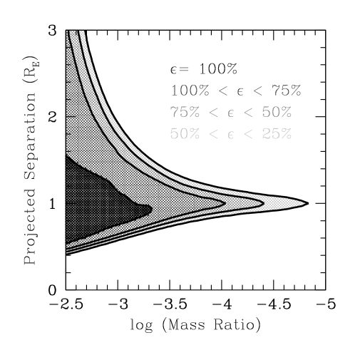
No convincing planetary signal has yet been detected, though not all data have been analyzed thoroughly. However, by comparing models with and without planets for all possible source trajectories [13], the presence of massive planets within certain zones of angular separation from their parent lenses can be ruled out in very well sampled, high magnification events [16, 17] (Fig. 7). The accumulation of many such events will lead in the next few years to the detection of planets like our own Jupiter — or to meaningful constraints on the abundance of such planets in the Galaxy (Fig. 8).

Figure 7: Top: The PLANET collaboration I band light curve containing $\sim$400 points for event OGLE 98-BLG-14 does not differ obviously from that of a single lens. Bottom: Exclusion probability contours for planetary companions of given mass ratio and instantaneous separation (in Einstein radii) orbiting this microlens [16, 17]. Within the solid black region, the best model with a planet differs from that without a planet by $\Delta\chi^{2}>100$ for all source trajectories.

6 Planetary Microlensing in the VLT Era

Small planets are difficult to detect with any method; microlensing is no exception. Earth-mass planets are especially elusive because the angular size of the planetary caustics are smaller than a giant star in the Bulge. Thus, even if an earth-mass caustic directly transits a background giant, only a piece of source is significantly magnified; source resolution greatly dilutes the signal [18]. In order to detect such small planets, several obstacles associated with earth-mass microlensing anomalies must be overcome simultaneously, namely their: (1) rarity, (2) short duration, (3) typically small amplitude, and (4) near invisibility against giant sources. A successful program would thus need to monitor hundreds of dwarf or turn-off stars undergo microlensing in the Bulge, and to do so frequently and with high precision.

The 2.5m VST equipped with OmegaCAM, a 16K $\times$ 16K CCD detector spanning a 1 degree field of view, is expected to see first light on Paranal in 2001 as a survey telescope for the VLT. The excellent weather and median seeing (0^′′.65), large field, and possibility of immediate VLT follow-up could make the VST the most formidable microlensing machine of its era; simultaneous detection and monitoring of 10 – 20 on-going microlensing events in every bulge field would be possible. Detailed observing strategies and simulations for the VST remain to be worked out, but first estimates are encouraging. Assuming that 1% photometry on V=20 (I=19) turn-off stars can be achieved with 4-5 minute integrations in these very dense fields, and allowing for 30-50% lost time due to weather or poor seeing, continuous observations with the VST during “bulge season” could yield as many as $\sim$20 jovian and $\sim$2 terrestrial-mass planets per year — if every lens has one of each sort of planet in its lensing zone [19, 20]. Since this is unlikely to be the case, detected numbers will be smaller, but it is only by measuring how much smaller that we can determine the abundance of such planets in our Galaxy.

Since microlensing “selects” lensing stars by mass, not luminosity, very distant and dim stars can be probed for planetary systems. Furthermore, the selection is a weak function of mass, so all types of Galactic stars can be studied. Unfortunately, because the parent star is unseen, its mass and distance are unknown: generally stellar lenses are too close (mas) to the source to be resolved with normal imaging and too faint to be detected in a combined spectrum. Lens mass $M$ and distance ${D_{\rm OL}}$ are the scaling parameters that are required to translate the planetary mass ratio $q$ into a planetary mass $m_{p}$ and the normalized instantaneous separation $b$ into physical units such as AU (see Eq. 1). Without knowledge of the lens mass and distance, ensembles of events must be fit with reasonable Galactic models to derive statistical estimates for these quantities.

On the other hand, 8-10m telescopes offer the first hope to spectrally type the otherwise unseen microlenses so that their distance and mass can be determined directly. Because the source and lens star are likely to differ in both spectral type and radial velocity, high resolution spectra ($\lambda/\Delta\lambda=40000$) with large apertures are expected to detect the lens signal in composite spectra, even for lens-source contrasts of 4 magnitudes — allowing dwarf lenses to be discerned [21]. In order to make best use of the potential for scientific gain, the microlensing events should be identified in real time at the VST so that VLT spectra can be taken both at peak, when the magnified source spectral energy distribution will dominate, and nearer baseline, when the composite spectrum will reflect the unlensed fraction of light from source and lens. This ambitious goal of direct lens detection would open a new era for microlensing, and is a task that the VLT is especially well suited to tackle due to its flexible instrumentation and scheduling, proximity to the VST, and the excellent seeing conditions on Paranal. The speed with which VLT instrumentation can be made ready and the availability of service observing will make it ideal for other target-of-opportunity science as well, such as the monitoring of (1) caustic crossings for proper motion and limb-darkening measurements, (2) supernovae, and (3) gamma ray burst optical counterparts.

Figure 8: Estimated detection efficiency contours of 10, 50, and 90% for current microlensing searches for planets of given mass ratio and true orbital separation $a$ in units of AU. (The Einstein ring radius is taken to be 3.5 AU, appropriate to a solar type Bulge lens.) Also shown are expectations for a radial velocity planet search running for 5 and 10 years (solid lines) and requiring 3-$\sigma$ detections at limiting sensitivities of 3 and 10 m s^-1, respectively. Positions of Jupiter, Saturn and Uranus are shown for reference. Adapted from Sackett (1999).

As Fig. 8 makes evident, if a sufficient number of events can be monitored sufficiently well, current microlensing searches will contribute to our knowledge of jovian mass planets orbiting with true orbital separations comparable to and somewhat larger than that of our own Jupiter, complementing current radial velocity searches which are sensitive to (and finding!) jovian planets at smaller orbital radii ($\hbox to0.0pt{\lower 2.15277pt\hbox{$\sim$} \hss}{\raise 1.72218pt\hbox{$<$}}3\,$AU). The VLT (and VST) era may see a widening of the parameter space to which microlensing can contribute valuable information, especially by pushing the technique forward to lower masses while allowing an improved characterization of detected planetary systems through better photometry and — possibly — direct spectroscopic microlens detection.

Acknowledgements

It is a pleasure to thank my colleagues in the PLANET collaboration for permission to display our results for OGLE 98-BLG-14 prior to publication, and Scott Gaudi for assistance in preparation of Fig. 8.

References

- [1]
- [2] Paczyński, B. (1986) Gravitational microlensing by the galactic halo. Ap.J. 304, 1-5.
- [3] Alcock, C., et al.: The MACHO Collaboration (1993) Possible gravitational microlensing of a star in the Large Magellanic Cloud. Nature 365, 621-22.
- [4] Aubourg, E., et al.: The EROS Collaboration (1993) Evidence for gravitational microlensing by dark objects in the galactic halo. Nature 365, 623-24.
- [5] Udalski, A., et al.: The OGLE Collaboration (1993) The optical gravitational lensing experiment. Discovery of the first candidate microlensing event in the direction of the Galactic Bulge. Acta Astron. 43, 289-294.
- [6] Mao, S. & Paczyński, B. (1991) Gravitational microlensing by double stars and planetary systems. Ap.J. 374, L37-40.
- [7] Griest, K. & Safizadeh, N. (1998) The Use of High-Magnification Microlensing Events in Discovering Extrasolar Planets. Ap.J. 500, 37-50.
- [8] Gaudi, B.S., Naber, R.M. & Sackett, P.D. (1998) Microlensing by Multiple Planets in High Magnification Events. Ap.J. 502, L33-37.
- [9] Wambsganss, J. (1997) Discovering Galactic planets by gravitational microlensing: magnification patterns and light curves. MNRAS 284, 172-188.
- [10] Dominik, M. (1999) The binary gravitational lens and its extreme cases. Submitted to Astron. Astrophys. (astro-ph/9903014)
- [11] Gould, A. & Loeb, A. (1992) Discovering planetary systems through gravitational microlenses. Ap.J. 396, 104-114.
- [12] Bolatto, A. & Falco, E. (1994) The detectability of planetary companions of compact Galactic objects from their effects on microlensed light curves of distant stars. Ap.J. 436, 112-116.
- [13] Gaudi, B.S. & Sackett, P.D. (1999) Detection Efficiencies of Microlensing Data Sets to Stellar and Planetary Companions. Submitted to Ap. J. (astro-ph/9904339)
- [14] Di Stefano, R. & Scalzo, R.A. (1999) A New Channel for the Detection of Planetary Systems through Microlensing. II. Repeating Events. Ap.J. 512, 579-600.
- [15] Albrow et al.: The PLANET Collaboration (1998). The 1995 Pilot Microlensing Campaign of PLANET: Searching for Anomalies through Precise, Rapid, Round-the-Clock Monitoring. Ap.J. 509, 687-702.
- [16] Gaudi et al.: The PLANET Collaboration (1998). Limits on Planetary Companions in Microlensing Event OGLE-BUL-98-14. AAS, 193, 108.07
- [17] Albrow et al.: The PLANET Collaboration (1999). In preparation.
- [18] Bennett, D. & Rhie, S. H. (1996) Detecting Earth-Mass Planets with Gravitational Microlensing. Ap.J. 472, 660-664.
- [19] Sackett, P.D. (1997) Planet Detection via Microlensing. Final Report of the ESO Working Group on the Detection of Extrasolar Planets. ESO SPG-VLTI-97/002, Appendix C (astro-ph/9709269)
- [20] Peale, S. J. (1997) Expectations from a Microlensing Search for Planets. Icarus 127, 269-289.
- [21] Mao, S., Reetz, J. & Lennon, D.J. (1998) Detecting luminous gravitational microlenses using spectroscopy. Astron. Astrophys. 338, 56-61.
- [22] Sackett, P.D. (1999) Searching for Unseen Planets via Occultation and Microlensing. Planets outside the Solar System: theory and observations, NATO-ASI Series, Kluwer, 189-227 (astro-ph/9811269)