The Hipparcos Transit Data: What, why and how?

Abstract

The Hipparcos Transit Data are a collection of partially reduced, fully calibrated observations of (mostly) double and multiple stars obtained with the ESA Hipparcos astrometry satellite. The data are publicly available, as part of the CD-ROM set distributed with the Hipparcos and Tycho Catalogues (ESA SP–1200, hip (1997)), for about a third of the Hipparcos Catalogue entries including all confirmed or suspected non-single stars. The Transit Data consist of signal modulation parameters derived from the individual transits of the targets across the Hipparcos focal grid. The Transit Data permit re-reduction of the satellite data for individual objects, using arbitrarily complex object models in which time-variable photometric as well as geometric characteristics may be taken into account. We describe the structure and contents of the Transit Data files and give examples of how the data can be used. Some of the applications use standard astronomical software: Difmap or AIPS for aperture synthesis imaging, and GaussFit for detailed model fitting. Fortran code converting the data into formats suitable for these application programs has been made public in order to encourage and facilitate the use of Hipparcos Transit Data.

1 Introduction

In the course of its three-year lifetime the European Space Agency’s Hipparcos satellite performed some 13 million scans across the $\sim\!118\leavevmode\nobreak\ 000$ stellar objects on its pre-defined observing list. For the vast majority of targets the subsequent data reductions succeeded in determining, accurately and without ambiguity, a small set of astrometric and photometric parameters which contain practically all the useful information on the objects. In the simplest case of a non-variable single star these data would be the position of the star at a certain epoch, the trigonometric parallax, the two proper motion components, a mean magnitude, and various statistics such as the mean errors of all the parameters. For thousands of variable, double and multiple stars, the necessary additional parameters were determined without too much problem. All of these results are readily available in the Hipparcos and Tycho Catalogues (ESA hip (1997)). For most objects and for most applications of the results, there is no need to probe deeper into the intricacies of the Hipparcos data acquisition and processing.

It was inevitable, however, that the observations of some (very small) fraction of the objects could not easily be interpreted in terms of standard models, and that inadequate, or even erroneous, object models were applied in some cases. Potentially very valuable information could have been lost for these objects if only summary results, based on inadequate models, were published. This situation has been avoided by including a good selection of intermediate results in the published catalogue. Being only partially reduced these results are less dependent on specific model assumptions, but still relatively simple to use thanks to a careful calibration into the photometric and astrometric systems of the final catalogue. The published version of the Hipparcos and Tycho Catalogues includes six CD-ROMs, five of which contain mainly such calibrated, partially reduced data. The data fall in three distinct categories:

• purely photometric information: the Epoch Photometry, consisting of calibrated magnitudes for each transit of the targets across the field, allowing a posteriori analysis e.g. of stellar variability (van Leeuwen et al. photom (1997));

• purely geometric information: the Intermediate Astrometric Data, which are the one-dimensional coordinates (‘abscissae’) of the targets on reference great circles, each coordinate derived from several consecutive transits and referring to a (Hipparcos-specific) centroid of the target (van Leeuwen & Evans hipi (1998));

• combined photometric and geometric information: the Transit Data (TD), which are the Fourier coefficients (equivalent to amplitude and phase) of the light modulation of the individual transits for each of the targets across the $0\aas@@fstack{\circ}9\times 0\aas@@fstack{\circ}9$ main grid of the Hipparcos instrument.

These mission products are fully described in Sects. 2.5, 2.8 and 2.9 of Vol. 1 of the Hipparcos and Tycho Catalogues. Examples using the Intermediate Astrometric Data have been given by van Leeuwen & Evans (hipi (1998)).

While the TD thus provide information that is more detailed and on a more fundamental level (in the sense of being closer to the satellite ‘raw’ data) than either the Epoch Photometry or the Intermediate Astrometric Data, two important restrictions should be noted: (1) TD are only available for about a third of the targets, or some 38 000 objects; (2) TD are based solely on the results from one of the data reduction consortia, the Northern Data Analysis Consortium (NDAC; Lindegren et al. ndac (1992)). By contrast, the Epoch Photometry and the Intermediate Astrometric Data are available for virtually all the 118 204 catalogue entries, and results from both NDAC and the Fundamental Astrometry by Space Techniques Consortium (FAST; Kovalevsky et al. fast (1992)) were normally used.

Detailed satellite operations and data reductions are described elsewhere (e.g., Perryman & Hassan vol1 (1989); Perryman et al. vol3 (1989); Perryman et al. mission (1992); Kovalevsky et al. fast (1992); Lindegren et al. ndac (1992); Vols. 2–4 of ESA hip (1997); van Leeuwen floor (1997)). It will however prove useful to review how the TD were measured in order to understand their precise meaning (and limitations), aiding in the full exploitation of the information. Thus, Sect. 2 describes the convolution of the stellar diffraction image with the modulation grid, and the resulting detector signal modeled by the TD. Section 3 is a detailed description of the contents and format of the published TD files. Two applications of the TD using publicly available software are demonstrated, viz. aperture synthesis imaging (Sect. 4) and model fitting (Sect. 5).

2 What are the Transit Data?

2.1 Availability of the data

The TD are contained on a CD-ROM (Disk 6) in Vol. 17 of the Hipparcos and Tycho Catalogues. A formal description of the TD, including detailed format specifications of the CD-ROM files, is found in Vol. 1, Sect. 2.9, of the Hipparcos and Tycho Catalogues. The TD come from an intermediate step of the data reductions performed by NDAC. In previous publications, the equivalent intermediate NDAC data were referred to as ‘Case History Files’ (Söderhjelm et al. ss92 (1992)). The data represent the scans (transits) of a selected number of targets from the Hipparcos Catalogue (HIP), comprising 37 368 systems with 38 535 different HIP entries. (Some systems have two or three HIP entries; cf. Fig. 2.) All Hipparcos stars that were classified as double, multiple or suspected non-single are included in the TD. Also, stars having problematic solutions in the Hipparcos Catalogue are included in the data set. In order to provide reference objects for calibrations or comparisons, several thousand ($\sim 5\,000$) ‘bona fide’ single stars were also included in the TD.

2.2 The modulated detector signal

The physical layout of the Hipparcos optical instrument was a telescope with two viewing directions in a plane perpendicular to the satellite’s spin axis. The two different fields of view were combined onto a single focal surface by a special combining mirror. The light from each program star within either field of view was focused onto the modulation grid, which was located in the focal surface.

The modulation grid consisted of a series of opaque and transparent bands. As the satellite spun, the diffraction image of each star traversed the grid perpendicular to the bands, resulting in a periodic ($\simeq 7$ ms period) modulation of the light intensity behind the grid. The varying intensity was measured by the Image Dissector Tube (IDT), a photomultiplier with an electronically steerable sensitive spot (‘Instantaneous Field of View’, IFOV) of about 30 arcsec diameter. During each ‘interlacing period’ of $\simeq 130$ ms the IFOV would cycle through the programme stars located within the $0\aas@@fstack{\circ}9\times 0\aas@@fstack{\circ}9$ field of view. There were on average 4 to 5 programme stars within the field of view at any given time.

The telescope entrance pupil (for each of the two viewing directions) was semi–circular, with diameter 0.29 m and with some central obscuration. The Airy radius of the (ideal) diffraction image was thus around 0.5 arcsec for an effective wavelength of 550 nm. The modulation grid had a basic period of 1.2074 arcsec, i.e. the separation between the centres of adjacent transparent bands (slits). The slit width was about 0.46 arcsec, well matched to the Airy disk size and representing a compromise between a sharp intensity maximum (requiring narrow slits) and high photon throughput (requiring wide slits).

Since the grid was periodic, the detector signal, being the convolution of the diffraction image with the grid transmittance, must also be a periodic function of the image centroid coordinate on the grid. Disregarding noise and variations in detector sensitivity, etc., the signal therefore consisted of a constant (DC) component plus modulated components having spatial frequencies that are integer multiples of the fundamental grid frequency. However, from the convolution theorem it follows that the signal cannot contain higher spatial frequencies than were already in the diffraction image. The maximum frequency in the diffraction image is given by the maximum separation of any two points in the pupil and the minimum detected wavelength ($\simeq 350$ nm). For a pupil diameter of 0.29 m this gives a spatial period of 0.25 arcsec. Thus the theoretically highest frequency in the signal is four cycles per grid period (the ‘fourth harmonic’). The fourth and third harmonics, with cycles of 0.3–0.4 arcsec, are however very strongly damped by the slit width (0.46 arcsec), which causes an averaging over more than one cycle for these components. As a result, the detector signal in practice contains only the first and second harmonics, in addition to the DC (mean intensity) component. Given the spatial frequency, the detector signal is therefore completely parametrized by five numbers, i.e. the DC term and the coefficients of the first two harmonics in the Fourier series representing the periodic signal. Furthermore, since Poisson (photon) noise is by far the dominating noise source for most Hipparcos observations, it can be shown that a proper estimate of these five Fourier coefficients constitutes a sufficient statistic for the further estimation of the photometric and geometric characteristics of the target, independent of its complexity. The TD contain precisely these Fourier coefficients along with the spatial frequencies and other ancillary data. From the viewpoint of statistical estimation, practically no information was therefore lost by compressing the raw photon counts (on average some 4500 bytes per transit and target) into the five Fourier coefficients (included in the TD file).

The detector signal thus measured certain components of the diffraction image moving over the modulation grid. The diffraction image, of course, had aberrations due to the imperfections of the telescope and chromatic effects caused by the wavelength-dependent diffraction. Also, the sensitivity of the IDT varied across the field and over the time. All of these factors affected the detector signal. The user of the TD need not worry about this, because the TD have been ‘rectified’, which means all instrumental and colour effects have been removed as far as possible by means of the various calibrations produced in the data reductions. Therefore, the TD should represent the response of an idealized, constant, and well-defined instrument to the object.

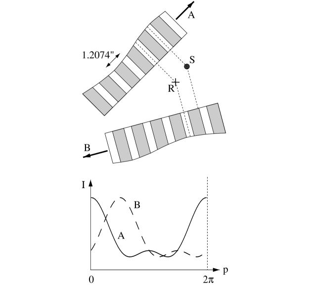
Figure 1: This figure illustrates the definition of reference phase $p$ (as in Eq. 1) by means of the reference point R on the sky (with specified astrometric parameters). $p=0$ at the instant when a slit is exactly centred on the reference point. In the lower diagram the curves A and B show the detector signal, as function of reference phase, produced by the same point source S when scanned in different directions. The intensity maximum is displaced from $p=0$ depending on the separation of S and R as projected on the grid, modulo the grid period 1.2074 arcsec.

2.3 The reference point

One of the key points of the TD is that the modulation phase in each scan is expressed with respect to a well-defined reference point on the sky. The astrometric parameters for the reference point (different for each target) are also specified in the TD. Usually the reference point corresponds to the data given in the Hipparcos Input Catalogue (HIC; Turon et al. hic (1992)). However, the phase calibration of the TD was made as if the coordinates of the reference point were expressed in the Hipparcos reference frame (nominally coinciding with the International Celestial Reference System, ICRS; Feissel & Mignard icrs (1998)). The phase offset of the TD from the reference point thus gives the differential correction to the position from the reference point in the ICRS system.

The reference point in general has its own values for proper motion and parallax, in addition to position. These values are contained in the TD ‘header record’, see Sect. 3.2.1. Of course, the real star also has a position, proper motion, and parallax. These two points move independently on the sky, according to their respective proper motion and parallax. In a particular transit the phase is determined by the scan direction and the distance between the two stars perpendicular to the slits. Figure 1 illustrates how the phase varies in two different scans across the star (S) and reference point (R). In scan A the star is in phase with the reference point, producing a light maximum for $p=0$ (and more generally for $p=n2\pi$, where $n$ is an integer). Scan B has the star out of phase with the reference point, resulting in a light maximum about a third of a period later ($p\simeq 2$ rad).

The raw detector signal consists of a sequence of photon counts, $N_{k}$, $k=1,2,\dots\,$, obtained in successive samples of $1/1200$ s integration time. The counts represent an underlying deterministic intensity modulation which (after background subtraction and various calibrations) is modeled as

$$I_{k}=b_{1}+b_{2}\cos{p_{k}}+b_{3}\sin{p_{k}}+b_{4}\cos{2p_{k}}+b_{5}\sin{2p_{k}}$$ (1)

where $b_{1}$–$b_{5}$ are the Fourier coefficients given in the TD. $I_{k}$ is the expected stellar count rate in sample $k$ (expressed in photons per sample of $1/1200$ s) and $p_{k}$ is the reference phase of the sample. The reference phase is defined by the following two conditions (cf. Fig. 1): (1) that $p_{k}=0$ if a slit is exactly centred on the reference point at the mid-time of sample $k$; and (2) that $p_{k}$ is increasing from 0 to $2\pi$ over the time it takes the grid to move one grid period (1.2074 arcsec) over the reference point.

Equation (1) is the most general representation of the signal produced by any object. In order to interpret this signal in terms of an object model it is necessary to know what the signal would be for a point source of unit intensity; in other words, we need the equivalent of the point-spread function in image processing. The rectification mentioned in Sect. 2.2 meant that the expected signal from a point source of magnitude $\mbox{\it Hp}=0$ (in the Hipparcos photometric system) located at the reference point is:

$$I_{k}=K[1+M_{1}\cos{p_{k}}+M_{2}\cos{2p_{k}}]\,.$$ (2)

Here $K=6200$ counts per sample, $M_{1}=0.7100$ and $M_{2}=0.2485$ are constants chosen not far from the actual mean calibration values at mid-mission (see Figs. 14.4, 14.3 and 5.6 in Vol. 3 of ESA hip (1997)).

2.4 Spatial frequencies

As illustrated by Fig. 1 the resulting signal will depend on the direction of scanning, even in the simple case of a point source with a fixed position relative to the reference point. The direction of scanning across the reference point can be specified by a position angle $\theta$ defined in the usual way, i.e. with $\theta=0$ for a scan where the grid is moving in the direction of increasing $\delta$ (‘North’), and $\theta=90^{\circ}$ for a scan in the direction of increasing $\alpha$ (‘East’). The spatial frequency of the grid, $f$ (expressed in radians of modulation per radian on the sky), is nominally $(1296000\leavevmode\nobreak\ \mbox{arcsec})/(1.2074\leavevmode\nobreak\ \mbox{arcsec})\simeq 1\,073\,400$. In reality it varies slightly, mainly because of differential stellar aberration, which changes the apparent scale by up to $\pm 0.01$ per cent depending on the barycentric velocity vector of the satellite. For the production of the TD data, the apparent scale and orientation of the grid, as projection onto the sky in the vicinity of the reference point, were strictly calculated for each transit, taking into account aberration as well as the satellite attitude and the calibrated field-to-grid geometric transformation. The result is expressed as the rectangular components of the spatial-frequency vector in the tangent plane of the sky:

$$f_{x}=-f\sin\theta\,,\qquad f_{y}=-f\cos\theta\,.$$ (3)

The minus signs mean that the spatial-frequency vector ($\@vec{f}$) points in the opposite direction to the motion of the grid across the reference point. This is purely a matter of convention, which was adopted for historic reasons.

2.5 The phase of an arbitrary point source

Consider now a point source of magnitude Hp which, in a particular scan, is displaced by $(x,y)$ from the reference point, where $x$ is measured positive towards increasing $\alpha$ and $y$ towards increasing $\delta$. Given the spatial frequency components of the scan, $f_{x}$ and $f_{y}$, the expected signal is:

$$I_{k} = 10^{-0.4{\it Hp}}K[1+M_{1}\cos(p_{k}+\phi)+M_{2}\cos 2(p_{k}+\phi)]$$

where

$$\phi=f_{x}x+f_{y}y$$ (5)

is the phase shift on the grid caused by the positional offset. [That $\phi$ is added to $p_{k}$ in Eq. (LABEL:eq:ikphi), rather than subtracted, is consistent with the sign convention adopted in the definition of $f_{x}$ and $f_{y}$.]

Equations (LABEL:eq:ikphi)–(5) are based on a linearization of the transformation between spherical coordinates and their projection on the tangent plane of the sky through the reference point. Within angular radius $\rho$ of the reference point, the neglected non-linear terms are generally of order $\rho^{3}$, or $<0.1$ mas for $\rho<160$ arcsec. Since the TD for a given target are normally confined to an area set by the size of the IDT sensitive spot ($\sim 30$ arcsec), or a few times this area (for multiple pointings), the linearization is always adequate.

The positional offset $(x,y)$ is in general caused by a time-dependent combination of the differences between the astrometric parameters of the star and of the reference point. The differences in $\alpha$, $\delta$, $\mu_{\alpha*}$ and $\mu_{\delta}$ are easily converted to an offset which is a linear function of time. The parallax difference produces a shift which is more complicated to calculate, as it depends on the position ($\@vec{s}$) of the satellite relative to the solar system barycentre at the time of observation. To facilitate this calculation, a third spatial frequency component, $f_{p}$, is supplied with the TD. This is basically just the scalar product $-\@vec{s}^{\prime}\@vec{f}$, where the satellite position $\@vec{s}$ is in astronomical units and $\@vec{f}$ is the previously defined spatial-frequency vector of the grid. With this definition it is found that a parallax difference of $\Delta\pi$ relative to the reference point causes the additional phase shift $\Delta\phi=f_{p}\Delta\pi$ in Eq. (5). The complete expression for the phase of a star with astrometric parameters $(\alpha,\delta,\pi,\mu_{\alpha*},\mu_{\delta})$ is therefore

$$\phi=f_{x}(\Delta\alpha{*}+t\Delta\mu_{\alpha*})+f_{y}(\Delta\delta+t\Delta\mu_{\delta})+f_{p}\Delta\pi$$ (6)

where $t$ is the time of the transit, expressed in (Julian) years from J1991.25, and $\Delta\alpha{*}=(\alpha-\alpha_{0})\cos\delta_{0}$, $\Delta\delta=\delta-\delta_{0}$, $\Delta\pi=\pi-\pi_{0}$, $\Delta\mu_{\alpha*}=\mu_{\alpha*}-\mu_{\alpha*0}$, $\Delta\mu_{\delta}=\mu_{\delta}-\mu_{\delta 0}$ are the differences with respect to the astrometric parameters of the reference point, $(\alpha_{0},\delta_{0},\pi_{0},\mu_{\alpha*0},\mu_{\delta 0})$.

The periodicity of the grid means that, in a given scan, positional differences that are multiples of the grid period in the direction of scanning will not produce measurable differences in the detector signal. This ‘grid-step ambiguity’ is normally resolved by the combination of scans from a variety of directions in the course of the mission.

2.6 Changing the reference point

The choice of reference point for the Transit Data is arbitrary, as long as it is sufficiently near the target for linearization errors to be negligible ($\la 160$ arcsec; see Sect. 2.5). As mentioned previously, the adopted reference point usually corresponds to the HIC values. The user may ask why the final astrometric parameters in the Hipparcos and Tycho Catalogues were not used instead. There were several reasons for this. First of all, the TD were derived directly from intermediate files of the NDAC reduction (Sect. 2.1), which were compiled in their final version almost a year before the astrometric parameters of the Hipparcos Catalogue became available. Secondly, most of the objects are double or multiple, and it is not evident which point to use in such cases. Finally, TD are available also for cases where no valid astrometric solution is provided in the Hipparcos Catalogue. In those cases it would have been necessary to use something like the HIC data anyway. Although it would have been possible, using the formulae below, to transform the TD to some other, possibly more natural or desirable reference point, such a process would in the end have been largely arbitrary. In addition, since any manipulation of the data always entails some risk of error, however small, it was felt better to leave the reference points as defined in the NDAC intermediate data files. The only modification applied was the transformation from the intermediate NDAC reference frame into the ICRS system, which was deemed essential; this was achieved by rotating the positions and proper motions of the reference points, rather than modifying the TD coefficients. (This explains why the position and proper motion of the reference point never coincide exactly with the HIC values.)

In some circumstances it may be desirable to change the reference point for a set of TD. This is particularly relevant for the construction of aperture synthesis images (Sect. 4), where the reference point defines the centre of the image. An object with a poorly determined pre–Hipparcos position may be severely offset from the centre of the reconstructed map, possibly falling outside the map altogether or creating a false image due to aliasing from a position outside the map. Not only the positional offset, but also errors in the proper motion and parallax of the reference point may create problems for the image reconstruction. The effect of such errors will be a blurring of the image due to the relative motion between the reference point and the true object. The proper motion error produces a blurring along a straight line in the map while the parallax error causes an additional elliptical blurring. Most objects with large proper motions ($>$ 100 mas yr^-1) or parallaxes ($>$ 100 mas) have reasonable, non-zero estimates of these quantities in the Input Catalogue, so the blurring effect is usually not very serious for qualitative evaluation of the images. However, for a quantitative analysis the effect needs to be considered.

Changing the astrometric parameters of the reference point requires that the phase of each transit is adjusted to take into account the apparent positional offset of the new reference point from the old one at the time of the transit. Fortunately, this is easily done by means of the spatial frequency components $f_{x}$, $f_{y}$, $f_{p}$ provided for each transit. Let $\Delta\alpha*=(\alpha_{0}^{\prime}-\alpha_{0})\cos\alpha_{0}$, $\Delta\delta=\delta_{0}^{\prime}-\delta_{0}$, etc., be the (small) differences between the new (^′) and the old reference point in terms of the five astrometric parameters. The required phase shift for a particular transit is then given by Eq. (6). The corresponding transformation of the Fourier coefficients in Eq. (1) is

$$b_{1}^{\prime} = b_{1}\,,$$

$$b_{2}^{\prime} = b_{2}\cos\phi-b_{3}\sin\phi\,,$$

$$b_{3}^{\prime} = b_{2}\sin\phi+b_{3}\cos\phi\,,$$ (7)

$$b_{4}^{\prime} = b_{4}\cos 2\phi-b_{5}\sin 2\phi\,,$$

$$b_{5}^{\prime} = b_{4}\sin 2\phi+b_{5}\cos 2\phi\,.$$

An example of the change of reference point is shown in Figs. 6 and 7.

2.7 Multiple pointings and target positions

One complication in the Hipparcos satellite operation and data reductions was caused by double and multiple stars having separations roughly in the range 10 to 30 arcsec. As already mentioned, the main Hipparcos detector had a sensitive area (IFOV) of about 30 arcsec diameter. This area could be directed towards any pre-defined point on the sky currently within the telescope field of view. The IFOV pointing, calculated from the real-time knowledge of the satellite attitude and the celestial position of the target, typically had errors of 1 to 2 arcsec rms. Ideally, no star should be observed while its image was close to the edge of the IFOV, where the guiding errors might produce a distorted signal. For double and multiple systems with separations less than about 10 arcsec this could be achieved by centering the IFOV somewhere in the middle of the system, so that all components remained within the flat-topped central part of the IFOV sensitivity profile. For systems with separations greater than about 30 arcsec the individual components (or subsystems with separations below 10 arcsec) could be observed as single stars, again avoiding signal distortion from the IFOV edges.

However, systems with intermediate separations ($\simeq 10$ to 30 arcsec) could not be observed without some adverse effects of the IFOV edges. In order to allow at least some useful astrometric information to be extracted for such systems, each component (or subsystem) received a separate pointing. For example, HIP 70 and HIP 71 formed such a two-pointing system with a separation of about 15 arcsec. When pointing at the brighter star (HIP 71, $Hp\simeq 8.4$), the other component (HIP 70, $Hp\simeq 10.6$) would be just at the edge of the IFOV and a (variable) fraction of its signal was added to that of the brighter star. Conversely, when pointing at the fainter component, some fraction of the brighter star’s signal would be added. Proper reduction of such systems must consider the mutual (and possibly distorted) influence of each component upon the other, as was indeed done in the Hipparcos data reductions. In some multiple systems three different pointings were needed.

The situation is further complicated by the fact that the targeted position of the IFOV was sometimes updated in the course of the mission, usually because the original (ground-based) position was found to be wrong by several arcsec. Knowledge of both the original and the updated position, and the time of updating, may then be necessary for proper interpretation of the observations.

In order to cope with two- and three-pointing systems as well as updated positions, the concept of ‘target positions’ was introduced in the TD. For a set of TD referring to a particular double or multiple system, target positions are defined by their offset coordinates $(\Delta\alpha*,\Delta\delta)$ from the adopted reference point, rounded to the nearest arcsec. In most cases there is just one target position, coinciding with the reference point [offset coordinates $=(0,0)$]. For multiple-pointing systems there is at least one target position for each pointing, with a different HIP number attached to each pointing. For objects whose coordinates relative to the reference point changed in the course of the mission, a new target position was introduced whenever the offset coordinates changed by more than 1 arcsec. To within the errors of the real-time attitude determination (normally 1–2 arcsec rms) it can therefore be assumed that the IFOV was pointed to the specified target position.

In the TD the results from different pointings pertaining to the same system have been collected together and expressed relative to a common reference point. This has been done for all systems deemed to be ‘difficult’ in the sense explained above, but not for very wide systems where the mutual influence of the component signals was negligible. The TD moreover contains the bookkeeping data necessary to calculate the actual target positions in each transit.

Table 1: Summary of the contents of the TD index and data files on Disk 6 of the Hipparcos Catalogue. Data fields in the Transit Data File are separated by the character ‘$|$’. In the header record there are 13 fields designated JH1 through JH13, etc.

Transit Data Index File (hip_j.idx)
120 416 records, each of 7 bytes+CR+LF = 9 bytes
The $n$th record in this file points to the header record
for HIP $n$ in hip_j.dat (Fig. 2)
Transit Data File (hip_j.dat)
4 351 156 records, each of 125 bytes+CR+LF = 127 bytes
The data for a given entry consist of one header record,
one pointing record, and $N_{T}$ transit records.
Header Record:
JH1–3	HIP identifiers (JH2–3 = 0 if not used)
JH4	$N_{P}$ = number of target positions
JH5	$N_{T}$ = number of transit records
JH6–10	$\alpha_{0}$, $\delta_{0}$, $\pi_{0}$, $\mu_{\alpha*0}$, $\mu_{\delta 0}$ = reference point
JH11–13	assumed colour indices ($V\!-\!I$) for JH1–3
Pointing Record:
JP1	index (1 to 3) to JH1–3 for target position 1
JP2	offset in $\alpha$ for target position 1 (arcsec)
JP3	offset in $\delta$ for target position 1 (arcsec)
JP4–6	same as JP1–3 but for target position 2
$\cdots$	$\cdots$
JP25–27	same as JP1–3 but for target position 9
Transit Record:
JT1	$I_{P}$ = target position (1 to $N_{P}$) for the transit
JT2	$t$ = epoch of the transit (years from J1991.25)
JT3–5	$f_{x}$, $f_{y}$, $f_{p}$ = spatial frequencies
JT6	$\ln b_{1}$
JT7–10	$b_{i}/b_{1}$, $i=2\dots 5$
JT11–15	$\ln\sigma_{i}$, $i=1\dots 5$ (standard errors of $b_{i}$)
JT16–17	$s_{1}$, $s_{2}$ = colour correction factors
JT18	$\sigma_{\rm att}$ = additional attitude noise (mas)
JT19	computed (0) or assumed (1) standard errors

3 The Transit Data files

This section gives a rather detailed description of the contents of the TD files, complementing the formal description in Vol. 1 of ESA (hip (1997)) and providing additional explanation of the data items. All relevant data are contained in two ASCII files, both located on Disk 6 in Vol. 17 of ESA (hip (1997)): the TD index file (hip_j.idx, $\simeq 1$ Mb) and the TD file (hip_j.dat, $\simeq 553$ Mb). A summary of the contents of the two files is in Table 1, while important relations among the data are illustrated in Fig. 2.

3.1 The index file: hip_j.idx

The TD index file is included to facilitate accessing the TD file. It contains a pointer from the HIP number to the corresponding record in the TD file where data on that object can be found. Since HIP numbers range from 1 to 120416, there are exactly 120416 records in the index file. Each record consists of a 7-character integer, which is the record number in the TD file for the relevant header record (Sect. 3.2.1). For example, TD for the double star HIP 7 can be accessed by first reading record number 7 in the index file (hip_j.idx). The content of that record is the integer 129. Record number 129 in the TD file (hip_j.dat) is thus the header record for HIP 7, and information on that object is contained in that and subsequent records of the TD file. If no TD are available for a given HIP number, then the corresponding index file record contains the number $-1$.

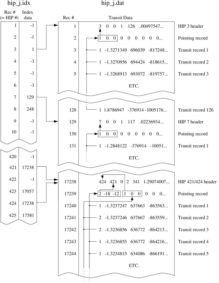
Figure 2: Relations among the contents of the index and data files.

For two- and three-pointing systems (Sect. 2.7) there are two or three different index file entries pointing to the same TD record. An example is shown in Fig. 2, where the index file entries for HIP 421 and HIP 424 both point to the 17238th record in the TD file.

For efficient accessing of the TD it is recommended that the index file is read into computer prime memory as a one-dimensional integer array of length 120416. This array is then used as a look-up table for finding data in the TD file. The TD file has a constant record length of 127 bytes (including the two end-of-record characters $\backslash$r$\backslash$n = CR+LF), which allows simple direct access to any given record number.

3.2 The TD file: hip_j.dat

3.2.1 The header record

The header record is the first record in the TD file containing data on a specific system. The index file always points to this header record for a given HIP number. The header record contains general information about the system in 13 data fields. In holding to the Hipparcos Catalogue conventions, the 13 data fields in the header record will be called JH1, JH2, $\dots\;$, JH13.

The first three data fields (JH1–3) contain the HIP numbers relevant to the subsequent transit records. JH1 is always defined; JH2 and JH3 are only defined for two- and three-pointing systems (Sect. 2.7). The number of pointings, or more accurately the number of different target positions ($N_{P}$), is specified in field JH4. Details on the relative pointings are given in the pointing record (Sect. 3.2.2).

JH5 gives the number of transits ($N_{T}$), or observations, for a given system. Since there is one record for each transit, this is also the number of transit records. The total number of records for an object is then $N_{T}+2$, where the header and pointing records make up the extra two records.

JH6–JH10 give, in order, the right ascension (deg), declination (deg), parallax (mas), proper motion in right ascension (mas yr^-1) and proper motion in declination (mas yr^-1) of the reference point. The Fourier coefficients $b_{1}$–$b_{5}$ of the subsequent transit records are expressed relative to this reference point. It is important to realize that these values are usually derived from the Input Catalogue and therefore do not agree with the astrometric parameters given in the Hipparcos Catalogue. For instance, the parallax of the reference point is often zero. The position refers to the epoch J1991.25, which was close to mid mission. The reference system is the same as that of the Hipparcos Catalogue, viz. the International Celestial Reference System (ICRS) (Feissel & Mignard icrs (1998)).

JH11–JH13 hold the assumed colour index $V\!-\!I$ (mag) for each of the three HIP numbers in JH1 through JH3. This value $V\!-\!I$ was used in rectifying the signals from each transit.

3.2.2 The pointing record

The pointing record defines the offset of the target position of each subsequent transit with respect to the reference point. The pointing record may define several different target positions as required for multiple-pointing objects. The actual number of different target positions ($N_{P}$) is given in JH4 of the header record. Each target position is specified by three numbers: the first takes the value 1, 2 or 3, depending on which of the HIP numbers in JH1, JH2 or JH3 that the target position refers to. The second and third numbers give the offset in $\alpha$ and $\delta$, respectively, of the target position from the reference point. These last two values are rounded to the nearest arcsecond.

Because every record of the TD file has 125 bytes, this allowed up to nine different target positions to be defined in the pointing record. In reality the maximum $N_{P}$ was 7.

Most objects used a single pointing, and the astrometric values in the Input Catalogue were sufficiently accurate that no updating was required. Moreover, the Input Catalogue values were usually taken as the reference point for the transit data. In this case $N_{P}=1$ and the first and only entry in the pointing record contains the three values: ‘1 0 0’ (cf. the excerpts for HIP 3 and 7 in Fig. 2). The ‘1’ refers to the HIP number in JH1. The ‘0 0’ means that the target position coincided (to the nearest arcsec) with the reference point. Subsequent transit records have ‘1’ in the first field (JT1) indicating that the target position for each transit was as given in the first entry of the pointing record.

In the trivial case of a single, well-centered pointing, as illustrated by HIP 3 and 7 above, the pointing record is really not needed. However, for those objects with multiple HIP entries and pointings, the pointing data provide important information. This is exemplified by the excerpt for the two-pointing system HIP 421$+$424 shown in the lower part of Fig. 2. As indicated in the header record, there are 341 transits for this system, made using two different target positions. The first transit for this system (in record 17240) was made with the IFOV pointing at the first target position (‘2  –18  –12’), i.e. referring to the second HIP entry (421) and pointing 18 arcsec to the west and 12 arcsec to the south of the reference point. The next transit (record 17241) was made in the second pointing (‘1 0 0’), i.e. referring to the first HIP entry (424) and centred on the reference point. The third transit (record 17242) was also made in the second pointing, while the fourth transit was made in the first pointing, and so on.

The fact that Hipparcos had two fields of view, separated by the ‘basic angle’ of $58^{\circ}$, is largely irrelevant for the use of the TD. There is in fact no flag in the TD telling in which field of view a particular transit occurred.

3.2.3 The transit data record

The actual scan information is contained in the transit data record. This section will cover the entries contained in these records, as well as some physical interpretations.

The first field (JT1) for each record tells which of the $N_{P}$ (= JH4) target positions was used to observe the transit. The second field (JT2) gives the time of the observation, in years, from the epoch J1991.25. The time is measured in Julian years of exactly 365.25 days. The epoch J1991.25 is equivalent to the Julian date JD 2 448 349.0625 on the Terrestrial Time (TT) scale.

The next three entries (JT3 to JT5) contain the spatial frequencies $f_{x}$, $f_{y}$ and $f_{p}$ defined as in Sects 2.4 and 2.5. They are expressed in units of rad rad^-1 (radian of modulation phase on the grid per radian on the sky).

The entries JT6 through JT10 contain, in coded form, the five Fourier coefficients $b_{1}$–$b_{5}$ defined by Eq. (1). JT6 contains the natural logarithm of $b_{1}$ ($\ln{b_{1}}$) and JT7 to JT10 contain the normalized coefficients ($b_{2}$/$b_{1}$, $b_{3}$/$b_{1}$, $b_{4}$/$b_{1}$ and $b_{5}$/$b_{1}$). This coding was adopted because $b_{1}$, being the mean intensity of the signal, is always positive and spanning a wide range of values according to the magnitude of the object; $b_{2}$ through $b_{5}$, on the other hand, may have either sign but are always numerically smaller than $b_{1}$.

The next five entries (JT11–15) contain the natural logarithms of the standard errors ($\sigma_{1}$–$\sigma_{5}$) for each of the Fourier coefficients. JT19, the last entry in this record, is a flag for the standard errors. JT19 is normally set to zero. It is set to ‘1’ if the standard errors could not be computed in the normal way, but were estimated roughly from the standard errors of the other transits. A non-zero value in JT19 is thus a warning that the standard errors in JT11–15 should be treated with caution.

JT16–17 contain two colour correction factors, $s_{1}$ and $s_{2}$. As previously mentioned, the TD are rectified signals, i.e. corrected for calibrated variations in the geometric and photometric responses. Among the many factors that have been taken into account in this process are the colour effects with respect to position in the field of view and time variations of the photometric calibrations. These corrections depend on an assumed colour for the object, as given in JH11–13. If it should turn out that the assumed colour for a particular transit was considerably in error, $s_{1}$ and $s_{2}$ provide a possibility to correct (approximately) the Fourier coefficients accordingly. See Sect. 2.9.3 in Vol. 1 of the Hipparcos and Tycho Catalogues for details of the correction procedure.

The second to the last entry (JT18) deals with the errors in the attitude determination. The phase determination of each scan was basically limited by photon noise, but the standard errors in JT11–15 also contain a contribution from the along-scan attitude uncertainty. It turned out to be very difficult to treat the attitude errors rigorously in the TD, and as a result these errors were generally underestimated. JT18 contains an estimate of the additional attitude noise ($\sigma_{\rm att}$, in mas) required in order to derive, from the TD, astrometric standard errors that are consistent with the main processing of Hipparcos data.

3.2.4 Known errors in the Transit Data

After publication of the Transit Data CD-ROM, six cases of Fortran format overflow errors have been discovered in the file hip_j.dat. No useful data are lost because of the errors, but special measures may be needed to read the corresponding records. The interface programs described in Sect. 6 automatically correct these errors. Further details can be found at the Internet address given in Sect. 6.

4 Aperture synthesis imaging

The Hipparcos satellite was not designed for imaging and did not contain any imaging device such as a CCD camera. The combination of a modulating grid and the IDT, while well adapted to the observation of isolated point sources, was far from ideal for the observation of more complex resolved objects. As explained in Sect. 2.2 the grid essentially extracted two spatial frequencies (with periods 1.2074 arcsec and 0.6037 arcsec in the direction of each scan) of whatever intensity distribution was within the 30 arcsec sensitive spot. This is much more reminiscent of spatial interferometry than of normal optical imaging. In fact, the two harmonics of the detector signal correspond to the fringes produced by an object in two interferometers with baselines of 94 mm and 188 mm, respectively (assuming an effective wavelength of 550 nm). Image reconstruction techniques using interferometric observations have for a long time been standard in the radio astronomical community. It was therefore quite natural to apply these techniques to the Hipparcos data (Lindegren lind (1982); Quist et al. quist (1997)).

4.1 Mathematical foundation

Equation (LABEL:eq:ikphi) gives the signal for a point source located at the position $\@vec{r}=(x,y)$ relative the reference point. Now consider an extended object with the general brightness distribution $B(\@vec{r})$. Summing up the contributions to the detector signal from each element of the sky we find (apart from a constant scaling factor)

$$I(p) = \int\!\!\!\int S(\@vec{r})B(\@vec{r})[1+M_{1}\cos(p+\@vec{f}\cdot\@vec{r})$$ (8)

$$\qquad{}+M_{2}\cos(2p+2\@vec{f}\cdot\@vec{r})]\,{\rm d}^{2}\@vec{r}$$

where $S(\@vec{r})$ is the sensitivity profile of the instantaneous field of view. Introducing the Fourier transform

$$V(\@vec{f})=\int\!\!\!\int S(\@vec{r})B(\@vec{r})\exp({\rm i}\@vec{f}\cdot\@vec{r})\,{\rm d}^{2}\@vec{r}$$ (9)

we find that Eq. (8) can be written

$$I(p) = V(\@vec{0})+\mbox{Re}[V(\@vec{f})]M_{1}\cos p-\mbox{Im}[V(\@vec{f})]M_{1}\sin p$$ (10)

$$+ \mbox{Re}[V(2\@vec{f})]M_{2}\cos 2p-\mbox{Im}[V(2\@vec{f})]M_{2}\sin 2p\,.$$

Comparison with Eq. (1) shows that

$$V(\@vec{0}) = b_{1}\,,$$

$$V(\@vec{f}) = (b_{2}-\mbox{i}b_{3})/M_{1}\,,\quad V(-\@vec{f})=V^{\ast}(\@vec{f})\,,$$

$$V(2\@vec{f}) = (b_{4}-\mbox{i}b_{5})/M_{2}\,,\quad V(-2\@vec{f})=V^{\ast}(2\@vec{f})\,,$$ (11)

where the asterisk denotes the complex conjugate. Since $M_{1}$ and $M_{2}$ are conventional constants (Sect. 2.3) it is seen that a single transit defines the complex function $V$ in the five points $\@vec{0}$, $\pm\@vec{f}$, $\pm 2\@vec{f}$, of the spatial frequency plane. However, the conjugate symmetry of $V$ means that there are only three independent complex visibilities per transit. Successive transits of the same object are made at different spatial frequencies $\@vec{f}=(f_{x},f_{y})$ and in the course of the mission knowledge of the function $V$ is built up in a number of different points. To the extent that $S(\@vec{r})B(\@vec{r})$ remains constant over the mission, it may then be recoverable from $V$ using standard image reconstruction techniques.

In the context of radio interferometry and aperture synthesis, we may identify $V(\@vec{f})$ with the complex visibility function associated with the source brightness distribution $B(\@vec{r})$ and single-antenna reception pattern $S(\@vec{r})$ (Thompson et al. thom (1994)). The visibility function is usually expressed in terms of coordinates $(u,v)$ which give the projection of the interferometer baseline on the sky plane and are expressed in wavelengths. The relation to the TD spatial frequency components is simply

$$u=f_{x}/2\pi\,,\quad v=f_{y}/2\pi\,.$$ (12)

Our reference point is equivalent to the phase reference position used in connected-element radio interferometry (Thompson et al. thom (1994)), or to the strong reference point source (typically a quasar) used in phase-referenced VLBI observations (Lestrade et al. lestr (1990)).

The distribution of the observations in the $uv$ plane is all-important for the possibility to reconstruct complicated images from the measured visibilities $V(u,v)$. Unfortunately the Hipparcos scanning law and the use of a modulating grid with just a single period seriously limit the $uv$ coverage of the TD. According to Eqs. (3) and (12) the coverage is limited to the central point $(u,v)=(0,0)$ and two concentric rings with radii $\simeq 170\,830$ and $341\,660$ wavelengths. Moreover, for objects in the ecliptic region of the sky (ecliptic latitude $|\beta|\la 45^{\circ}$) the scanning law constrains the scan angle $\theta$ such as to produce a gap of ‘missing’ scans roughly in the east–west direction. At $|\beta|\simeq 47^{\circ}$ there is instead a surplus of scans in the east–west direction (cf. Fig. 3). For high-latitude objects, finally, the coverage is usually more uniform in $\theta$.

In continuing the analogy with radio interferometry, we will discuss in the next section how images can be produced using the Transit Data. Utilizing the experience developed for aperture synthesis imaging, we use only publicly available software for producing and deconvolving these images.

4.2 Conversion of TD to UV-FITS format

The images presented here were produced using the Caltech Difmap software package (Shepherd shep (1997)). Another software package that could be used for the analysis is AIPS (Astronomical Image Processing System) developed at the National Radio Astronomy Observatories (NRAO). Both Difmap and AIPS take input data in the form of FITS files, using the ‘Random Groups’ format (NOST nost2 (1994)). This amendment to the basic FITS format is more commonly called the UV-FITS format, since it is used almost solely for interferometry data.

We have written and made publicly available (Sect. 6) a concise Fortran program which reads TD from the CD-ROM format (hip_j.idx and hip_j.dat) for any given object and produces an output file in the UV-FITS format. In the following we describe some of the features of the UV-FITS format and how the TD were adapted to it.

The basic FITS (Flexible Image Transport System; Wells et al. fits1 (1981); NOST nost1 (1993)), well known in optical astronomy, was designed to transport digital data in the form of $n$-dimensional regular arrays, such as CCD images, with associated information on coordinates, dates, scales, units, etc. given in an ASCII header. However, aperture synthesis visibility data do not come in regular arrays, at least not in all axes, and thus an amendment to the basic FITS was required allowing the definition of ordered sets of small arrays (Greisen & Harten fits2 (1981)). In the following we assume that the reader has some rudimentary knowledge about the basic FITS format.

In a UV-FITS file each random group contains the visibility data associated with a particular point in $uv$ space and time. The group consists of a set of parameters followed by a regular array of measurements. The parameters are, for instance, the $uv$ coordinates and date of the measurements. The measurement array may be multi-dimensional with, for instance, the different frequencies and Stokes (polarization) components marked along two of the axes. In the UV-FITS header the use of random groups is signified by having a first axis of length zero (${\tt NAXIS1}=0$) and by setting the keyword ${\tt GROUPS}={\tt T}$ (true). Visibility data are stored as three values in the measurement array, namely the real part of the visibility, the imaginary part, and an associated weight. In the array, this corresponds to an axis of length 3 and type ${\tt COMPLEX}$.

For the Hipparcos TD there are three visibility measurements per transit, corresponding to the spatial frequencies $\@vec{0}$, $\@vec{f}$ and $2\@vec{f}$. The total number of random groups is therefore ${\tt GCOUNT}=3N_{T}$. ${\tt PCOUNT}=6$ parameters specify each group, namely the Fourier coordinates $(u,v,w)$, the baseline (defining which pair of antennae that formed the interferometer), and the date of the observation (split in two numbers containing the integer and fractional parts of the Julian date). For the TD the $w$ coordinate is always zero.

The UV-FITS format requires that the $(u,v)$ coordinates are expressed in seconds, while in Eq. (12) they are dimensionless. The conversion factor requires the specification of a reference wavelength, for which we arbitrarily adopted $\lambda_{0}=550$ nm. The corresponding scale factor for the $(u,v)$ coordinates in Eq. (12) is then ${\tt PSCAL1}={\tt PSCAL2}=\lambda_{0}/c$, where $c$ is the speed of light. For consistency, the frequency associated with each TD observation must then be given as $c/\lambda_{0}$.

The measurement array in each group is 5-dimensional (${\tt NAXIS}=6$, since the first axis has zero length for group data). Its size is ${\tt NAXIS2}\times{\tt NAXIS3}\times{\tt NAXIS4}\times{\tt NAXIS5}\times{\tt NAXIS6}=3\times 1\times 1\times 1\times 1=3$, where the axes are of type ${\tt COMPLEX}$, ${\tt STOKES}$, ${\tt FREQ}$, ${\tt RA}$ and ${\tt DEC}$, respectively. The values on each axis are specified in the header by ${\tt CRVAL}n$ for $n=2\dots 6$; in particular the frequency is given by ${\tt CRVAL4}=c/\lambda_{0}$ and the reference position by ${\tt CRVAL5}=\alpha_{0}$ and ${\tt CRVAL6}=\delta_{0}$. The three values in the measurement array are, as mentioned before, the real and imaginary parts of $V(u,v)$ and an associated weight. For the TD the weight is always equal to $1$.

The aperture synthesis programs also require the names and geocentric positions of the antenna stations to be specified, although this is rather pointless in our case. We formally specify six stations and identify a different pair with each spatial frequency. The stations are arbitrarily named to form the acronym ‘HIPUVF’, which will appear on some plots.

An apparent limitation of the FITS format is the lack of keywords for proper motion and parallax. Until such keywords become standard, the proper motions and parallax values of the reference point are given in the ASCII header as comments.

Figure 3: UV coverage for HIP 97237. For every point $(u,v)$ marked in this diagram there is a measurement of the complex visibility $V$ representing the amplitude and phase of the detector signal during a certain transit. Each transit provides five equidistant visibilities (including the origin) oriented along a straight line through the origin. The celestial orientation of the line is normal to the slits of the Hipparcos modulation grid at the transit. $u$ is the spatial frequency in the east–west direction, expressed in modulation periods (‘wavelengths’) per radian on the sky; $v$ is the north–south component of the spatial frequency in the same unit.

4.3 Example images

Once the data are converted into a suitable form, images are quickly produced using standard aperture synthesis programs. Using the Difmap package from Caltech (Sect. 6), we give here as an example a reduction of the TD for HIP 97237. In the Hipparcos Catalogue, no astrometric solution is given for this relatively faint ($V\simeq 12.4$) object. In the Hipparcos Input Catalogue it is noted as a double star (CCDM 19458+2707) with separation 0.9 arcsec and component magnitudes 12.7 and 13.6. The ecliptic latitude of the object is $\beta\simeq+47^{\circ}$. The reference point for this object is $\alpha_{0}=296.43849356$ deg, $\delta_{0}=+27.12735771$ deg, $\pi_{0}=97.00$ mas, $\mu_{\alpha*0}=-25.43$ mas yr^-1, $\mu_{\delta 0}=-1228.86$ mas yr^-1.

Figure 3 shows the UV-coverage of HIP 97237. It is seen that the object received rather many scans, although predominantly in the (ecliptic) east–west direction. The ‘dirty beam’ (Fig. 4) reflects this anisotropy as a characteristic pattern along the east–west section, reminiscent of the basic light modulation curve in Fig. 1.

Figure 4: The dirty beam (point spread function) associated with the UV coverage of HIP 97237 shown in Fig. 3.

Figure 5: The dirty map of HIP 97237, obtained by an inverse Fourier transform of all the measured complex visibilities.

The ‘dirty map’, basically obtained as the inverse Fourier transform of the complex visibilities, is shown in Fig. 5. Already from this image it is obvious that the object was offset from the expected (HIC) position by about 5 arcsec. This is probably the reason why an acceptable solution was not found in the Hipparcos astrometric reductions. Deconvolution of the dirty image, using the dirty beam as kernel (point spread function), can be achieved by means of the CLEAN algorithm (Högbom clean (1974)) implemented in Difmap. One result of this process (which depends on several parameters selectable in Difmap) is shown in Fig. 6. Both components of the double star are now clearly seen. The offset of the primary component from the reference point, estimated from the cleaned image, is $(\Delta\alpha*,\Delta\delta)\simeq(+3.6,+3.6)$ arcsec. The position of the secondary component relative to the primary is approximately 0.9 arcsec towards position angle $330^{\circ}$. The power in the primary peak of the cleaned map is 0.0455 units, where 6200 units corresponds to magnitude $Hp=0$ (Sect. 2.3); the magnitude of the primary can thus be estimated at $Hp\simeq 12.8$.

Figure 7 illustrates the change of reference point for the TD described in Sect. 2.6. The astrometric parameters of the primary component in HIP 97237, relative to the reference point, were estimated by means of the model fitting procedure described in Sect. 5. The approximate results were (cf. Fig. 9) $\Delta\alpha*=+3603$ mas, $\Delta\delta=+3640$ mas, $\Delta\pi=-16$ mas, $\Delta\mu_{\alpha*}=-50$ mas yr^-1, $\Delta\mu_{\delta}=-25$ mas yr^-1. Applying the corresponding phase shifts to the TD, according to Eqs. (6) and (2.6), effectively changes the reference point to coincide with the primary component. Performing the image synthesis on the modified TD gives the cleaned image in Fig. 7. As expected, the primary now appears at the centre of the map. The shift in parallax and proper motion of the reference point improves the relative phasing of the superposed scans, resulting in a slightly increased peak power (from 0.0455 to 0.0457 units).

Figure 6: The cleaned map of HIP 97237, obtained by deconvolution of Fig. 5 with the beam in Fig. 4. The cleaned map clearly reveals the two components of the double star.

Figure 7: The cleaned map of HIP 97237 resulting from modified TD, in which the astrometric parameters of the reference point were shifted to coincide with the astrometric parameters of the primary component. determined using the model fitting procedure described in Sect. 5.

5 Model fitting

The aperture synthesis imaging attempts to reconstruct the brightness distribution on the sky, in principle without making any a priori assumption about the object. This is excellent for exploring cases where the nature of the object is uncertain, e.g. concerning the number of resolved components in a multiple star or their approximate positions. The method is less useful for accurate quantitative evaluation, in particular because the offsets in parallax and proper motion merely produce a blurring of the image. Since the objects of interest here consist of a small number of point sources, direct modeling of the TD in terms of simple superposed signal components is usually possible. Such model fitting provides the most direct and accurate estimates of specific object parameters such as the trigonometric parallax or orbital elements. In this section we outline the fitting procedure and give an example of its practical realization by means of a publicly available computer program.

5.1 General method

Let us assume that the object consists of $n$ point sources with intensities $A_{j}$ and positions $x_{j}$, $y_{j}$ relative the reference point ($j=1\dots n$). In general $A_{j}$, $x_{j}$, $y_{j}$ vary with time, and so may be different for the different transits of the same object. Given a specific model of the object we express $A_{j}$, $x_{j}$, $y_{j}$ as functions of time $t$ and a set of model parameters $\@vec{a}$. For instance, in the case of a non-variable orbital binary, $\@vec{a}$ would consist of 15 parameters, viz. the five astrometric parameters of the mass centre, the magnitude of each component, the mass ratio, and seven elements for the relative orbit. Generally speaking, the object model is thus completely specified by $n$ and the functions $A_{j}(t,\@vec{a})$, $x_{j}(t,\@vec{a})$, $y_{j}(t,\@vec{a})$ for $j=1\dots n$. In the equations below we suppress, for brevity, the explicit dependence on $t$ and $\@vec{a}$.

For a given transit the expected signal is modeled as the sum of the signals from the individual components, using Eqs. (LABEL:eq:ikphi) and (5). Thus,

$$I_{k} = \sum_{j=1}^{n}A_{j}[1+M_{1}\cos(p_{k}+f_{x}x_{j}+f_{y}y_{j})$$ (13)

$$\qquad{}+M_{2}\cos 2(p_{k}+f_{x}x_{j}+f_{y}y_{j})]\,.$$

Expanding the trigonometric functions and equating the terms with those in Eq. (1) yields

$$b_{1} = \phantom{-M_{1}}\sum_{j}A_{j}\,,$$

$$b_{2} = \phantom{-}M_{1}\sum_{j}A_{j}\cos(f_{x}x_{j}+f_{y}y_{j})\,,$$

$$b_{3} = -M_{1}\sum_{j}A_{j}\sin(f_{x}x_{j}+f_{y}y_{j})\,,$$ (14)

$$b_{4} = \phantom{-}M_{2}\sum_{j}A_{j}\cos 2(f_{x}x_{j}+f_{y}y_{j})\,,$$

$$b_{5} = -M_{2}\sum_{j}A_{j}\sin 2(f_{x}x_{j}+f_{y}y_{j})\,.$$

Recall that $A_{j}$, $x_{j}$, $y_{j}$ depend on the model parameters $\@vec{a}$. The general procedure is then to adjust $\@vec{a}$ in such a way that, for the whole set of transits, the calculated signal parameters $b_{1}$–$b_{5}$ from Eq. (14) agree, as well as possible, with the observed values. The adjustment may use the weighted least-squares method, using the standard errors of the observed signal parameters to set the weights; but other (and more robust) metrics can also be used. In general the problem can be formulated as a constrained minimization problem in the multi-dimensional model parameter space.

The trigonometric functions in Eq. (14) mean that the signal parameters $b_{i}$ depend in a highly non-linear manner on the model parameters which affect $x_{j}$ and $y_{j}$. For instance, in terms of a displacement of one of the point sources, the effect on $b_{4}$ and $b_{5}$ is approximately linear only for displacements less than about $1/2f\simeq 0.1$ arcsec, corresponding to 1 rad change in the modulation phase. In the aperture synthesis imaging this non-linearity is manifest in the complex structure of the ‘dirty beam’ (Fig. 4) at all spatial scales larger than about 0.1 arcsec. Additional non-linearities in the complete object model may result from the geometrical description of the source positions, e.g. in terms of orbital elements.

The non-linearity of the object model has two important consequences for the model fitting. Firstly, it is usually necessary to use a non-linear, iterative adjustment algorithm, such as the Levenberg–Marquardt method (Press et al. nr2 (1992)). Secondly, a good initial guess of the model parameters is usually required. In particular the parameters directly affecting the positions of the point sources need to be specified to within (what corresponds to) a few tenths of an arcsec. Without a good initial guess, the adjustment algorithm is likely to converge on some local minimum, typically resulting in positional errors of (approximately) an integer number of grid periods. The correct solution, corresponding to the global minimum, may in principle always be found through sufficiently extensive searching of the parameter space. Alternatively, sufficiently good initial guesses of the point source positions can often be obtained from the aperture synthesis imaging.

Various least-squares model fitting procedures were used for the reduction of double and multiple stars during the construction of the Hipparcos Catalogue (see Mignard et al. mign (1992) and references therein). The double-star processing of the NDAC data reduction consortium (Söderhjelm et al. ss92 (1992)) essentially used the technique outlined above, taking the so-called Case History Files (a precursor to the TD) as input.

Perhaps the greatest potential of the TD lies in the possibility to combine the Hipparcos data with independent observations from other instruments and epochs. For instance, full determination of a binary orbit generally requires data covering at least a whole period. Ground-based speckle observations can sometimes provide this, constraining the geometry of the relative orbit much better than the Hipparcos data alone, and in turn leading to a better-determined space parallax. In some favourable cases the location of the mass centre in the relative orbit (and hence the mass ratio) can be determined (Söderhjelm et al. ss97 (1997); Söderhjelm ss99 (1999)).

One complication of the Hipparcos double star processing has been the wide variety of applicable object models, and the consequent need to experiment and interact with the solutions. This process may be much facilitated by using general and flexible software for the model fitting, rather than highly specialized routines. An example of this is given below.

5.2 Model fitting using GaussFit

GaussFit (Jefferys et al. 1988a , 1988b ) is a general program for the solution of least squares and robust estimation problems, developed as a platform to facilitate astrometric reduction of data from the Hubble Space Telescope. It is written in the C programming language and may thus be run under a variety of operating systems. In this section we outline the use of GaussFit for model fitting to the TD, again using the binary HIP 97237 as illustration.

GaussFit was used by Söderhjelm (ss99 (1999)) in a systematic re-examination of the solutions for several double and multiple objects, through a combination of TD with ground-based observations. Although not illustrated in the example below, the introduction of additional data (e.g. relative positions from speckle observations) is quite straightforward by means of GaussFit.

To run GaussFit, the user must supply several input files. During execution these files are read (and sometimes modified) by GaussFit, and additional output files generated. For application to the TD model fitting the following input files are required.

• The data file: this contains the observational data, in our case the TD. A special program (td2uv.f) is available (Sect. 6) to extract the TD for a given HIP number and format them as required by GaussFit. The resulting data file consists of 16 columns and one data line per transit. The columns contain a sequential number for the transit, the target position index (JT1), the time of the transit, the spatial frequencies $f_{x}$, $f_{y}$, $f_{p}$, the signal parameters $b_{1}$–$b_{5}$ and their variances. The header of the data file defines the name of the variable associated with each column.

• The model file (cf. Fig. 8): this is a mathematical description of the object model written in the GaussFit programming language. This language is modeled on C, but includes some specific constructs. For instance, the declaration of variables distinguishes between ‘observations’ (input data with random errors that need to be taken into account in the fitting), ‘data’ (error-free input data), ‘parameters’ (to be adjusted by the program), and ordinary ‘variables’. The special function $\tt import()$ reads one line of data from the data file. The function $\tt export(x)$ sends the equation of condition $x=0$ to the estimation algorithm, taking into account the uncertainties of the observational data that went into calculating $x$.

• The parameter file: this contains the initial guesses of all the model parameters to be estimated. On output it contains the estimated parameter values and estimated errors.

• The environment file contains general information needed for the model fitting, such as the names of the data, parameter and output files; the type of estimation algorithm to be used (standard least squares or a robust method), and stopping rules for the iterations.

The reader is referred to the GaussFit User’s Manual (Jefferys et al. 1988b ) for detailed information.

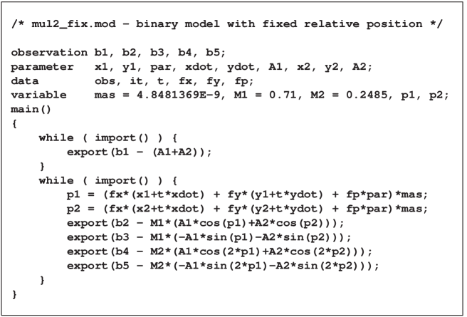
Figure 8: An example of a double-star model defined in the GaussFit programming language.

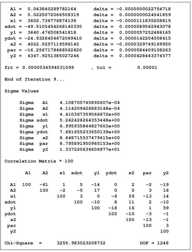
Figure 9: Part of the GaussFit output (slightly edited) obtained while fitting the double star model in Fig. 8 to the TD for HIP 97237.

Figure 8 is an example of a GaussFit model file. It describes a binary with a fixed positional offset between the components (i.e. a long-period binary). The model parameters are thus the astrometric parameters of the primary relative to the reference point (${\tt x1}=\Delta\alpha*_{1}$, ${\tt y1}=\Delta\delta_{1}$, ${\tt par}=\Delta\pi$, ${\tt xdot}=\Delta\mu_{\alpha*}$, ${\tt ydot}=\Delta\mu_{\delta}$), the position of the secondary relative to the reference point (${\tt x2}=\Delta\alpha*_{2}$, ${\tt y1}=\Delta\delta_{2}$); and the intensities of the components, ${\tt A1}=A_{1}$, ${\tt A2}=A_{2}$. The components are assumed to have the same parallax and proper motion. The expressions within the $\tt export()$ functions are easily recognized as the equations of condition, Eq. (14), written in terms of the model parameters. The five $\tt export()$ statements are divided among two $\tt import()$ loops (which means that the data file is forced to be read twice in each iteration): the reason is that GaussFit in its standard distribution version cannot handle more than four simultaneous equations of condition.

The model in Fig. 8 was applied to the TD of HIP 97237, using as starting approximation (3600, 3600, 0, 0, 0, 0.04, 4000, 4300, 0.02) for the variables in the parameter list (cf. Sect. 4.3). The ‘fair’ metric with an asymptotic relative efficiency of 0.95 was used for robust estimation of the parameters (Jefferys et al. 1988a ). Part of the output file, containing the results of the final (10th) iteration, is shown in Fig. 9. It should be noted that the estimated standard errors (sigma values) given in the output file have already been scaled by $(\chi^{2}/\nu)^{1/2}$, using the chi-square ($\chi^{2}$) and degrees of freedom ($\nu$) given at the end of the file. Adding the results of the model fitting to the reference point data (Sect. 4.3) and using the magnitude conversion formula $Hp=-2.5\log(A/K)$ we obtain the following estimated parameters of the binary HIP 97237 (ICRS, epoch J1991.25):

$$\alpha_{1} = 296.43961803\leavevmode\nobreak\ \mbox{deg}\pm\phantom{0}4.41\leavevmode\nobreak\ \mbox{mas}\,,$$

$$\alpha_{2} = 296.43974889\leavevmode\nobreak\ \mbox{deg}\pm\phantom{0}8.65\leavevmode\nobreak\ \mbox{mas}\,,$$

$$\delta_{1} = \phantom{0}27.12836895\leavevmode\nobreak\ \mbox{deg}\pm\phantom{0}7.00\leavevmode\nobreak\ \mbox{mas}\,,$$

$$\delta_{2} = \phantom{0}27.12856546\leavevmode\nobreak\ \mbox{deg}\pm 13.37\leavevmode\nobreak\ \mbox{mas}\,,$$

$$\pi = \phantom{-00}80.74\pm 8.80\leavevmode\nobreak\ \mbox{mas}$$

$$\mu_{\alpha*} = \phantom{00}\mbox{$-74.94$}\pm 5.24\leavevmode\nobreak\ \mbox{mas\leavevmode\nobreak\ yr}^{-1}\,,$$

$$\mu_{\delta} = -1203.93\pm 7.68\leavevmode\nobreak\ \mbox{mas\leavevmode\nobreak\ yr}^{-1}\,,$$

$$Hp_{1} = 12.88\pm 0.01\leavevmode\nobreak\ \mbox{mag}\,,$$

$$Hp_{2} = 13.60\pm 0.02\leavevmode\nobreak\ \mbox{mag}\,.$$

These data are in reasonable agreement with the values derived by Söderhjelm (ss99 (1999)) in an orbital solution combining the TD with ground-based speckle observations.

6 Software availability

Fortran programs interfacing the TD with aperture synthesis software and with GaussFit are available via the Lund Observatory Internet address http://www.astro.lu.se/$\sim$lennart/TD/. The program td2uv.f extracts the TD for a given HIP identifier and converts them into a UV-FITS file that can be used e.g. by Difmap. The program td2gf.f similarly extracts TD data and generates a data file suitable as input for GaussFit. Sample data files, additional information on the TD (including descriptions of the known errors), and links for retrieving aperture synthesis software and GaussFit are also given at this site.

7 Conclusions

The Hipparcos Transit Data, published as part of the Hipparcos and Tycho Catalogues (ESA hip (1997)), provide data from an intermediate step in the data reduction process of the NDAC data analysis consortium. Transit Data are given for all known or suspected double or multiple star systems in the Hipparcos Catalogue, or about a third of the objects in the catalogue. There were several reasons to include these data in the published catalogue. A main reason was the realization that every stellar system could not be examined for every possible type of solution within the time available for completing the catalogue. Ideally, such examination should also take into account ground-based observations. The Transit Data allow the user to re-examine such solutions, should the need arise.

Basically the Transit Data contain the Fourier coefficients which describe the modulation of the detector signal caused by the object’s motion across the modulating grid. As such they retain all the photometric and astrometric information on the object gathered during its transit across the grid. The Transit Data have been carefully calibrated and referred to the Hipparcos photometric and astrometric systems, so that any data derived from them should be directly comparable with other results in the published catalogue.

By giving this review of how the Transit Data were recorded, what they physically represent and examples of their practical uses, we hope to encourage readers to utilize the data in their own exploitations of the Hipparcos results. To aid this process, we have made programs available which provide interfaces with publicly available software packages, in particular Difmap and GaussFit. Many other applications could be thought of – the combination of Transit Data with ground-based speckle observations of double stars to improve orbits, parallaxes and mass ratios by Söderhjelm (ss99 (1999)) is an example. What has been covered and demonstrated here might just be a stepping stone to new and creative exploitations of the Transit Data.

- (1) ESA 1997, The Hipparcos and Tycho Catalogues ESA SP–1200
- (2) Feissel M., Mignard F. 1998, A&A, 331, L33
- (3) Greisen E.W., Harten R.H. 1981, A&AS, 44, 371
- (4) Högbom J.A. 1974, A&AS, 15, 417
- (5) Jefferys W.H., Fitzpatrick M.J., McArthur B.E. 1988a, Celestial Mechanics 41, 39
- (6) Jefferys W.H., Fitzpatrick M.J., McArthur B.E., McCartney J.E. 1988b, GaussFit: A System for least squares and robust estimation, User’s Manual. Dept. of Astronomy and McDonald Observatory, Austin, Texas (75 pp)
- (7) Kovalevsky J., Falin J.L, Pieplu J.L., et al. 1992, A&A, 258, 7
- (8) van Leeuwen F., 1997, Space Sci. Rev. 81, 201
- (9) van Leeuwen F., Evans D.W. 1998, A&AS, 130, 157
- (10) van Leeuwen F., Evans D.W., Grenon M., et al. 1997, A&A, 323, L61
- (11) Lestrade J.-F., Rogers A.E.E., Whitney A.R., et al. 1990, AJ 99, 1663
- (12) Lindegren L., 1982, Imaging properties of Hipparcos and the Observation of Multiple Stars. in: M.A.C. Perryman, T.D. Guyenne (eds.) The Scientific Aspects of the Hipparcos Mission. ESA SP–177, p. 147
- (13) Lindegren L., Høg E., van Leeuwen F., et al. 1992, A&A, 258, 18
- (14) Mignard F., Söderhjelm S., Bernstein H., et al. 1995, A&A, 304, 94
- (15) NOST, Definition of the Flexible Image Transport System (FITS), 1993, NOST 100-1.0 (Greenbelt: NASA/Goddard Space Flight Center).
- (16) NOST, A user’s Guide for the Flexible Image Transport System (FITS), 1994, NOST Ver. 3.1 (Greenbelt: NASA/Goddard Space Flight Center).
- (17) Perryman M.A.C., Hassan H., 1989, The Hipparcos Mission Pre-Launch Status, Vol. I: The Hipparcos Satellite, ESA SP–1111
- (18) Perryman M.A.C., Lindegren L., Murray C.A., Høg E., Kovalevsky J. 1989, The Hipparcos Mission Pre-Launch Status, Vol. III: The Data Reductions, ESA SP–1111
- (19) Perryman M.A.C., Høg E., Kovalevsky J., et al. 1992, A&A, 258, 1
- (20) Press W.H., Teukolsky S.A., Vetterling W.T., Flannery B.P. 1992, Numerical recipes (2nd ed.). Cambridge Univ. Press, Cambridge
- (21) Quist C.F., Lindegren L., Söderhjelm S. 1997, Using Hipparcos Transit Data for Apeture Synthesis Imaging. in: B. Battrick (eds.) Hipparcos Venice 97, ESA SP–402, p. 257
- (22) Shepherd M.C. 1997, Difmap: An Interactive Program for Synthesis Imaging. In: Hunt G. and Payne H.E. (eds.) Astronomical Data Analysis Software and Systems VI, ASP Conference Series, Vol 125, p. 77
- (23) Söderhjelm S. 1999, A&A, 341, 121
- (24) Söderhjelm S., Evans D.W., van Leeuwen F., Lindegren L. 1992, A&AS, 258, 157
- (25) Söderhjelm S., Lindegren L., Perryman M.A.C. 1997, Binary Star Masses from Hipparcos. in: B. Battrick (eds.) Hipparcos Venice 97, ESA SP–402, p. 251
- (26) Thompson A.R., Moran J.M., Swenson G.W. 1994, Interferometry and Synthesis in Radio Astronomy, Krieger Publ. Co., Malabar, Florida
- (27) Turon C., Crézé M., Egret D., et al. 1992, The Hipparcos Input Catalogue, ESA SP–1136
- (28) Wells D.C., Greisen E.W., Harten R.H. 1981, A&AS 44, 363