The circumstellar envelope of AFGL 4106

Abstract

We present new imaging and spectroscopy of the post-red supergiant binary AFGL 4106. Coronographic imaging in H$\alpha$ reveals the shape and extent of the ionized region in the circumstellar envelope (CSE). Echelle spectroscopy with the slit covering almost the entire extent of the CSE is used to derive the physical conditions in the ionized region and the optical depth of the dust contained within the CSE.

The dust shell around AFGL 4106 is clumpy and mixed with ionized gas. H$\alpha$ and [N ii] emission is brightest from a thin bow-shaped layer just outside of the detached dust shell. On-going mass loss is traced by [Ca ii] emission and blue-shifted absorption in lines of low-ionization species. A simple model is used to interpret the spatial distribution of the circumstellar extinction and the dust emission in a consistent way.

1 Introduction

In their final stages of evolution, both massive ($M{\vbox{\hbox{$>$}\offinterlineskip\hbox{$\sim$}}}8$ M_⊙) and intermediate-mass ($1{\vbox{\hbox{$<$}\offinterlineskip\hbox{$\sim$}}}M{\vbox{\hbox{$<$}\offinterlineskip\hbox{$\sim$}}}8$ M_⊙) stars can become dust-enshrouded as a result of intense mass loss at rates of $10^{-5}$ up to $10^{-3}$ M_⊙ yr^-1. For the massive stars, this heavy mass loss occurs during the red supergiant (RSG) phase, while for the intermediate-mass stars this happens during the Asymptotic Giant Branch (AGB) evolution. After having lost a significant fraction of their initial mass during this episode, the photospheric temperature of the star increases again and the stellar ultraviolet (UV) radiation field starts ionizing the dusty CSE, producing either a Planetary Nebula (PN) or a post-RSG nebula surrounding a Wolf-Rayet star. The mechanisms at play during the short-lasting transition stage between RSG/AGB and WR/PN are still poorly known. Especially the final evolution of the massive objects is hitherto poorly documented. One such massive object is AFGL 4106.

García-Lario et al. (1994) discovered nebular line emission from the IR object AFGL 4106, which came as a surprise because the central star was thought to be of spectral type G: too cool to ionize a CSE. The dust shell around AFGL 4106 was imaged in the infrared (IR) by Molster et al. (1999) who modelled the spectral energy distribution as observed by ISO with a radiation transfer code. They provide evidence that the object is a binary consisting of a late-A/early-F type star and a somewhat fainter M-type companion. Their distance estimate yields luminosities too high for AGB evolution and hence AFGL 4106 must be the result of post-RSG evolution.

Here we present and analyse new observations of this object and focus on the spatial distribution and physical conditions of the CSE around AFGL4106. Coronographic imaging in H$\alpha$ shows the spatial distribution of the ionized material around AFGL 4106. Spatially resolved echelle spectroscopy is performed to measure expansion velocities, electron densities and the internal extinction by the dust. The spatial distribution of dust extinction and emission is modelled in a consistent way. Finally we discuss the structure of the circumstellar envelope and the recent mass-loss history of AFGL 4106.

2 Observations

2.1 H$\alpha$ coronographic imaging

On February 4, 1996, we used the multi-mode instrument EMMI at the ESO 3.5m NTT on La Silla, Chile, to image AFGL 4106 through a filter centred at H$\alpha$, with a rather narrow width of 33 Å to avoid contamination by [N ii] emission. Because of the high apparent brightness of the star (9^th mag in V) coronographic techniques were used to limit the saturation of the CCD. A glass plate was inserted in the aperture wheel, holding six dark blots of different size and attenuation. The star was placed behind a 1.9^′′ blot with a central attenuation of a few mag. Two frames of each 5 min integration time in H$\alpha$ were combined. A 10 s exposure through a broad-band Johnson R filter was used to correct for the continuum contribution within the H$\alpha$ filter band. The R-band image was aligned with the H$\alpha$ image and scaled linearly by comparing the intensities of several field stars. Before subtracting the R-band image from the H$\alpha$ image both were corrected for structure in the instrumental response over the pixels of the CCD by dividing them by images of the morning twilight sky, taken through the corresponding filters. Remaining CCD artifacts and cosmic ray impacts were removed by hand. The seeing was constant at 1^′′, and the pixel size was 0.268^′′.

2.2 Echelle spectroscopic imaging

On February 4, 1996, we used the same telescope and instrument to take echelle spectra of AFGL 4106 with several slit orientations. The wavelength region extended from 6000 to 8350 Å. Using a slit width of 1^′′ a resolving power of $R\sim 7.5\times 10^{4}$ was obtained corresponding to a velocity resolution of 4 km s^-1. The slit length was set to 15^′′ and the spatial resolution was 0.268^′′ per pixel. We centred the star in the middle of the slit but obtained 15 min spectra with different position angles: 0^∘, 45^∘, 90^∘ and 135^∘ where the position angle is defined from West over North. The reduction of the spectra was standard and included flat-fielding, wavelength calibration on the basis of Th-Ar exposures, spectral response correction on the basis of a measured spectrum of standard star HD 60753, interactive cosmic hit cleaning, extinction correction with average extinction values, and finally absolute flux calibration. The seeing was about 0.8 to 0.9^′′.

3 Results

3.1 H$\alpha$ coronographic imaging

Figure 1: Coronographic image in the light of H$\alpha$ on a logarithmic flux density scale. The flux density level of the brightest part of the extended emission is $\sim 7\times 10^{-15}$ W m${}^{-2}\mu$m^-1 arcsec^-2. The faintest emission visible in the picture is a factor of ten fainter. North is up, and East is to the left.

The coronographic image in H$\alpha$ is displayed on a logarithmic flux density scale in Fig. 1. North is up, and East is to the left. The star itself is heavily saturated despite the use of the coronographic blot, resulting in the artificial NS-orientated bar. The absolute flux density calibration was derived from the spectra and is estimated to be accurate within $\sim 20$%. The flux density level of the brightest part of the extended emission is $\sim 7\times 10^{-15}$ W m${}^{-2}\mu$m^-1 arcsec^-2. The faintest emission visible in the picture is about a factor of ten fainter.

AFGL 4106 appears to be situated in a bright, spatially extended emission complex. From N to W of the star, the strongest emission delineates a bow-shaped structure much akin the bow-shocks associated with stars that move supersonically through the interstellar medium (Kaper et al. 1997). The emission bow is located at a projected distance of 5^′′ up to 10^′′ from the central star. The faintest H$\alpha$ emission is detected up to $\sim 14^{\prime\prime}$ from the central star. In the SE much less H$\alpha$ emission is detected. Interestingly, the 10 $\mu$m emission (Molster et al. 1999) shows a clear anti-correlation with the H$\alpha$ emission: the 10 $\mu$m emission peaks in the SE and is faintest in the NW.

3.2 Echelle spectroscopic imaging

3.2.1 Absorption lines

The spectral type has been redetermined by van Winckel et al. (in preparation) and Molster et al. (1999). The optical spectrum is dominated by a late-A or early-F type star (T${}_{\rm eff}\sim 7500$ K) with a nitrogen-enhanced photosphere resulting in strong N i absorption lines around 8000 Å. They also spectroscopically discovered the presence of an early-M type companion star (T${}_{\rm eff}\sim 3750$ K). The self-absorbed H$\alpha$ line profile centred on the star is identical to that observed by García-Lario et al. (1994). This suggests that the H$\alpha$ emission conditions in the vicinity of the star have been stable over a period of at least six years.

Figure 2: Radial velocity curve for AFGL 4106. The solution is not unique, but periods much longer than 12 yr are difficult to reconcile with this data.

A total of 31 absorption lines of the atomic and singly ionized species Fe i, Fe ii, Sc ii, Si ii, O i, Mg ii, Na i and N i were selected for measuring the star’s radial velocity. Considering a heliocentric correction for the movement of the Earth of $+13.3$ km s^-1, the heliocentric velocity of the star is determined at $v_{\star}=+8.1\pm 0.7$ km s^-1. For an individual line, the typical deviation from the mean was 4 km s^-1, which is equal to the spectral resolution. The stellar velocity differs considerably from the value of $v_{\star}=-47\pm 2$ km s^-1 derived by García-Lario et al. (1994) from the Si ii $\lambda\lambda$6347,6371 lines (after transforming from LSR to heliocentre) in their spectra taken in February 1990. In March 1992, ¹²CO J=1$\rightarrow$0 emission at 115 GHz was detected by Josselin et al. (1998). From the mean of the velocities of the blue- and red-most CO emission we estimate $v_{\star}=-3\pm 1$ km s^-1. An additional measurement from photospheric absorption lines in high resolution spectra taken in July 1996 (van Winckel et al., in preparation) yields $v_{\star}=-4\pm 1.2$ km s^-1. An approximate radial velocity curve (Fig. 2) for the maximum period possible, assuming circular orbits, yields $P_{\rm max}=4500$ d. For (currently) equal masses of the two stars Kepler’s third law yields the mass of each star: $M\sim 15\sin^{-3}i$ M_⊙ with orbital inclination angle $i$ (shorter periods imply smaller masses).

Figure 3: Spectrum around Si ii $\lambda$6347 Å (solid) and the same spectrum mirrored with respect to 6347.29 Å where the line profile is deepest (dashed). Below, their difference spectrum is plotted. The wavelength axis is heliocentric.

The Si ii $\lambda\lambda$6347,6371, Fe ii $\lambda$6456, N i $\lambda$7468 and Fe i $\lambda$8327 absorption lines have asymmetric line profiles, with more absorption in the blue wing. This may be caused by outflowing matter due to present day mass loss. The spectrum around Si ii $\lambda$6347 is shown as an example (Fig. 3). The spectrum was normalised by dividing by a constant equal to the spectrum level outside of the absorption line, i.e. the spectral slope is not affected. Also plotted is the difference between this spectrum, and the spectrum after mirroring with respect to the absorption extremum at 6347.29 Å(after heliocentric correction). This difference spectrum shows the absorption excess in the blue wing of the line profile, reaching a maximum at a blueshift of $\sim 40$ km s^-1.

3.2.2 Diffuse Interstellar Bands and the $E(B-V)$

The centroid wavelengths and equivalent widths of 68 Diffuse Interstellar Bands (DIBs) were measured. These DIBs are found over the entire spectral coverage, although few are found at wavelengths longer than 7400 Å. The DIBs were identified using Jenniskens & Desert (1994), from which also the conversion factors between equivalent width and colour excess $E(B-V)$ for each DIB were adopted. The derived colour excess is $E(B-V)=0.9^{+0.2}_{-0.1}$ mag, confirming the estimated $E(B-V)=1.0\pm 0.2$ mag from a smaller selection of DIBs by Molster et al. (1999) to whom we refer for a thorough discussion on the distance to AFGL 4106. The heliocentric velocity is $v_{\rm DIB}=+3\pm 2$ km s^-1. The velocity of the DIBs differs significantly from both the velocity of AFGL 4106 as measured from the spectra as well as the system velocity of AFGL4106, confirming that the DIBs are of interstellar not circumstellar origin.

3.2.3 [N ii] emission lines

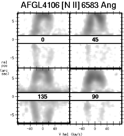
Figure 4: Spatial and kinematic map of [N ii] $\lambda$6583. The stellar continuum is subtracted, and the flux scale is logarithmic. The relative positions are defined as running from E to W at a position angle 0^∘, SE to NW at 45^∘, S to N at 90^∘ and SW to NE at 135^∘. The wavelength axes are transformed into heliocentric Doppler velocity axes.

The [N ii] $\lambda$6583 line is the strongest emission line in AFGL 4106, and the best tracer of the kinematics of the circumstellar nebula. Unlike the H$\alpha$, there is no stellar contribution to the line profile. The underlying stellar continuum is subtracted by scaling the spatial profile of the stellar spectrum outside the kinematic extend of the [N ii] emission. In this way a map is constructed of the [N ii] emission as a function of the position along the slit relative to the stellar position, and the heliocentric Doppler velocity, for each of the four slit orientations (Fig. 4). The flux scale is logarithmic, and the relative positions are counted from E to W (at 0^∘), from SE to NW (at 45^∘), from S to N (at 90^∘) and from SW to NE (at 135^∘). Close to the stellar position the stellar continuum was too dominant over the [N ii] emission to reliably correct for it, and this region in the four maps is covered by the labels with the slit position angles.

The maps of the [N ii] emission are consistent with emission from a radially expanding shell, with an expansion velocity of $\sim 30$ km s^-1 and a radius of $\sim 7^{\prime\prime}$. As in the H$\alpha$ emission map, the NW side is brighter than the SE side. The expansion velocity is smaller than the 40 km s^-1 derived from the Si ii absorption and also smaller than the $v_{\rm exp}=35\pm 1$ km s^-1 that we estimate from the ¹²CO J=1$\rightarrow$0 emission at 115 GHz detected by Josselin et al. (1998).

Figure 5: Spatial profile of [N ii] $\lambda$6583 (top panel), obtained by summing the spectra taken at the four different position angles, with the relative position defined as in Fig. 4. Positive relative positions roughly correspond to NW. The blue- and red-shifted emission is shown individually. The logarithm of their ratio yields the internal optical depth $\tau$ (bottom panel) under the assumption that the [N ii] emission arises from a spherically symmetric expanding shell.

The spectra at the four different position angles were summed and integrated over the blue- and red-shifted velocity range, respectively. This results in an effective cross section of the spatially extended emission complex running roughly from SE to NW, i.e. from the minimum to the maximum of the emission measure. The result is plotted in the top panel of Fig. 5. Assuming that the source of the [N ii] emission is a spherically symmetric expanding shell, the logarithm of the ratio of the blue- over the red-shifted emission corresponds to the optical depth within the emitting shell. This is because the red-shifted emission corresponds to the far side of the shell and has to traverse through the dusty CSE within the shell before it emerges at the observer’s side which is also where the blue-shifted emission arises from. The derived spatial profile of the optical depth is shown in the bottom panel of Fig. 5.

The optical depth profile traces the dusty CSE out to a radius of $5^{\prime\prime}$, which corresponds to the spatial extent of the 10 $\mu$m emission (Molster et al. 1999), to the inner boundary of the H$\alpha$ maximum (Fig. 1) and the forbidden line maxima (Fig. 4). The optical depth at $\lambda=6583$ Å exceeds unity at a distance of $\sim 2^{\prime\prime}$ from the star, but is lower closer to the star. This corresponds to the inner cavity also seen in the 10 $\mu$m emission. The red-shifted [N ii] emission becomes stronger than the blue-shifted emission at relative positions ${\vbox{\hbox{$>$}\offinterlineskip\hbox{$\sim$}}}5^{\prime\prime}$. This cannot be explained by optical depth effects and must therefore indicate deviations from spherical symmetry in the density and/or excitation conditions in that part of the nebula.

3.2.4 [S ii] emission lines

Figure 6: Spatial profile of [S ii] $\lambda$6717 and $\lambda$6731 (top panel), obtained as in Fig. 5 but integrated over the entire kinematic extent of the emission line. Their flux ratio is plotted in the bottom panel.

The [S ii] $\lambda\lambda$6717,6731 emission is co-spatial with the [N ii] emission, as seen from the spectra at the four different position angles. The spectra are summed in the same way as in preparing the [N ii] spatial profile in Fig. 5, but now the emission line is integrated over its entire kinematic extent. This results in one-dimensional spatial emission profiles for both components of the [S ii] doublet (Fig. 6, top panel). The emission peaks in the NW (positive relative position), where the H$\alpha$ is brightest too.

The ratio of the emission profiles of the 6717 and 6731 Å components (Fig. 6, bottom panel) may be used to derive the local electron density $n_{e}$ (Osterbrock 1988). For $n_{e}<100$ cm^-3 this ratio is $>1.3$, with a maximum of 1.42. For $n_{e}>10^{4}$ cm^-3 the ratio is $<0.5$, with a minimum of 0.44. This holds for an electron temperature of $T_{e}=10^{4}$ K. The derived electron density scales with $\sqrt{T_{e}}$. The CSE of AFGL 4106 outside of the region of 10 $\mu$m emission has $n_{e}<100$ cm^-3, whereas the inner CSE corresponding to the cavity in the 10 $\mu$m emission has $n_{e}>10^{4}$ cm^-3.

3.2.5 H$\alpha$ emission line

Figure 7: Spatial profiles of H$\alpha$ and [N ii] $\lambda\lambda$6548,6583, obtained as in Fig. 5 (top panel). Their flux ratio is plotted in the bottom panel.

Figure 8: Spatial profiles of H$\alpha$ and [S ii] $\lambda\lambda$6717,6731, obtained as in Fig. 5 (top panel). Their flux ratio is plotted in the bottom panel.

Spatial profiles of the H$\alpha$ emission were created in the same way as for [S ii]. The H$\alpha$ profile is compared with the profiles of [N ii] (Fig. 7) and [S ii] (Fig. 8).

The flux ratios of H$\alpha$ and forbidden lines are in the range $\log(F_{{\rm H}\alpha}/F_{\rm[N\ II]})\sim-0.3$ to $-0.05$ and $\log(F_{{\rm H}\alpha}/F_{\rm[S\ II]})\sim 0.3$ to $0.7$. This strongly suggests excitation conditions similar to those in Planetary Nebulae but different from those in H ii regions (García-Lario et al. 1991). The H$\alpha$ emission is co-spatial with the forbidden line emission. The H$\alpha$/[N ii] ratio seems smallest in the brightest part of the nebula around a relative position of $+5^{\prime\prime}$. The H$\alpha$/[S ii] ratio seems to be smallest close to the star. This effect may be caused by the spatial variation of the ratio of the [S ii] components, with the $\lambda$6717 component essentially following the H$\alpha$ emission.

3.2.6 Fe i and [Ca ii] emission lines

Though reported by García-Lario et al. (1994), 16.6 Å wide Fe i emission centred at 6380.7 Å could not be confirmed.

Figure 9: Spectrum around [Ca ii] $\lambda\lambda$7291,7324. The wavelength axes are transformed into heliocentric Doppler velocity axes.

Instead, weak fluorescence emission of the 1F doublet of [Ca ii] $\lambda\lambda$7291,7324 is detected (Fig. 9). The spectra have been normalised in the same way as the Si ii spectrum (Fig. 3). The emission is centred on the star and spatially unresolved. The line profiles are distorted due to the presence of numerous telluric absorption lines but appear to be kinematically symmetric with respect to the stellar velocity. The emission extends between about $\pm 20$ km s^-1, which is somewhat narrower than the H$\alpha$, [N ii] and [S ii] emission. The equivalent widths of the lines are $W_{7291}=-26\pm 3$ and $W_{7324}=-31\pm 4$ mÅ, respectively. The line profiles peak at a flux density (above the stellar continuum) of $F_{7291}\sim 3.0\times 10^{-12}$ and $F_{7324}\sim 2.3\times 10^{-12}$ W m${}^{-2}\mu$m^-1, respectively.

The location of the [Ca ii] emission can be further constrained by estimating where the outflow reaches the critical density for the [Ca ii] lines of $n_{\rm crit}=10^{7}$ cm^-3. However, this requires calculation of the mass-loss rate. The mass-loss rate may be estimated from the CO emission reported by Josselin et al. (1998). For the moment it is assumed that this mass-loss rate is valid for the unresolved inner regions of the nebula.

With distance $D$, outflow velocity $v$, CO abundance $f$ with respect to H₂, CO peak antenna temperature $T$, and a simplified model for the CSE (Kastner 1992), the total mass-loss rate can be derived:

$$\dot{M}=3.8\times 10^{-12} \left(\frac{T}{0.08}\right)^{\gamma}\times$$ (1)

$$\times\frac{D^{2}\left[{\rm kpc}\right]^{2}v^{2}\left[{\rm kms}^{-1}\right]^{2}}{f}{\rm M}_{\odot}{\rm yr}^{-1}$$

with the parameter $\gamma$ approximated as follows:

$$\gamma=\left\{\begin{array}[]{ll}\frac{1}{2}&\mbox{for $\dot{M}<10^{-7}$ M${}_{\odot}$ yr${}^{-1}$}\\ \frac{2}{3}&\mbox{for $10^{-7}<\dot{M}<10^{-6}$ M${}_{\odot}$ yr${}^{-1}$}\\ \frac{3}{4}&\mbox{for $10^{-6}<\dot{M}<10^{-5}$ M${}_{\odot}$ yr${}^{-1}$}\end{array}\right.$$ (2)

For higher mass-loss rates, more detailed modelling is required. In that case the CO line profile will become saturated, and hence it is no longer the peak antenna temperature, but the shape of the line profile that yields an estimate of the mass-loss rate. With $v=35$ km s^-1, $f=2\times 10^{-4}$, $T=0.14$ K, and $\gamma=\frac{3}{4}$, the mass-loss rate is obtained:

$$\dot{M}=3.5\times 10^{-5}D^{2}\left[{\rm kpc}\right]^{2}{\rm M}_{\odot}{\rm yr}^{-1}$$ (3)

This implies a very high mass-loss rate if the star were to be considerably more distant than one kpc, but still an order of magnitude less than the mass-loss rate derived by Molster et al. (1999) who estimate $\dot{M}\sim 3\times 10^{-4}D\left[{\rm kpc}\right]$ M_⊙ yr^-1.

The angular separation $d$ from the star from which the [Ca ii] emission arises can now be estimated assuming a constant outflow velocity of $v=35$ km s^-1, and an average particle mass of $2.7\times 10^{-24}$ g:

$$d=1.4\times 10^{13}D\left[{\rm kpc}\right]{\rm m}=0.09^{\prime\prime}$$ (4)

Hence for distances of $D{\vbox{\hbox{$<$}\offinterlineskip\hbox{$\sim$}}}20$ kpc the [Ca ii] emission must arise from well within the inner cavity that is seen in the 10 $\mu$m emission and in the internal extinction of the [N ii] emission. If the mass-loss rate in those inner regions is lower than the CO estimate, then the [Ca ii] emission is located even closer to the star. This is consistent with the [Ca ii] emission being spatially unresolved.

4 Modelling the circumstellar dust envelope

The dust around AFGL 4106 causes extinction of line emission that originates from behind the dusty CSE, and emission in the mid- and far-IR. Our spatially resolved spectra of the nebular line emission were used to construct a spatial profile of the optical depth of the dusty CSE, and the spatially resolved dust emission at 10 $\mu$m was published by Molster et al. (1999). Here we make an attempt to simultaneously model the spatial profiles of the optical depth and of the dust emission.

4.1 Circumstellar dust extinction

Suppose that the bulk of the H$\alpha$ and [N ii] emission originates from a region just outside the dusty envelope. The emission from the front and backside is observed at blue- and red-shifted velocities, respectively. Assuming equally strong front and backside emission, the ratio of the observed line flux at red- and at blue-shifted velocities directly yields the differential extinction experienced by the backside emission after traversing the dusty CSE. The [N ii] $\lambda$6583 line is best suited for this method because it is strong and its intrinsic width is small compared to the much larger thermal width of the H$\alpha$ line emission.

Figure 10: Schematic representation of the dust shell around AFGL 4106, and the coordinates used in the modelling.

The mass-loss rate history through the dusty CSE is parameterised as:

$$\dot{M_{r}}=\dot{M_{R}}\left(\frac{r}{R}\right)^{\alpha}$$ (5)

The case of $\alpha=0$ corresponds to a steady mass loss. The outflow velocity through the dusty CSE is assumed to be constant. The optical depth $\tau_{0.66}$ at 0.66 $\mu$m as a function of dimensionless projected distance $\Delta$ is:

$$\tau_{0.66}=\zeta g(\Delta)$$ (6)

where $\Delta=1$ at the outer radius $R$ of the dusty CSE, and $\Delta=\Delta_{0}$ at the inner radius $R_{0}$ of the dusty CSE (Fig. 10). The spatial profile of the observed optical depth has a shape:

$$g(\Delta)=\int_{x}^{1}\frac{y^{\alpha-1}}{\sqrt{y^{2}-\Delta^{2}}}{\rm d}y$$ (7)

with lower integration boundary:

$$x=\left\{\begin{array}[]{ll}1&\mbox{if $\Delta>1$}\\ \Delta&\mbox{if $\Delta_{0}<\Delta<1$}\\ \Delta_{0}&\mbox{if $\Delta<\Delta_{0}$}\end{array}\right.$$ (8)

and a scaling parameter:

$$\zeta=\frac{3\psi\dot{M_{R}}}{8\pi Rvs}\times\frac{Q_{0.66}}{a}$$ (9)

with dust-to-gas ratio $\psi=5\times 10^{-3}$, constant outflow velocity $v$, dust grain specific mass $s=3$ g cm^-3 and radius $a$, and extinction coefficient $Q_{0.66}=14a\left[{\mu}{\rm m}\right]$ for oxygen-rich dust (Volk & Kwok 1988).

Figure 11: Top panel: spatial profile of the optical depth $\tau$ at 0.66 $\mu$m as derived from the [N ii] $\lambda$6583 emission. Bottom panel: spatial profile of the 10 $\mu$m emission, for $p=1$. In both panels, calculated profiles are plotted for different mass-loss rate histories ($\alpha$, see text).

For $\alpha\in\left\{-2,-1,0,1,2\right\}$ the function $g$ can be evaluated analytically. To obtain a reasonable fit to the observed profile, the parameters $\Delta_{0}$, $R$ and $\zeta$ need to be tuned accordingly. The model profiles are convolved with a gaussian of $\sigma=0.36^{\prime\prime}$, corresponding to the Full Width at Half Maximum of the stellar continuum in the spatial direction ($0.85^{\prime\prime}$). We fitted by eye, aiming at equal maximum optical depth for all $\alpha$. The results are plotted in Fig. 11 (top panel) and summarised in Table 1.

4.2 Circumstellar dust emission

The spatial profile of the observed N-band flux density per square arcsecond can be calculated as follows:

$$F_{N}=\zeta^{\prime}g^{\prime}(\Delta)$$ (10)

with a shape:

$$g^{\prime}(\Delta)=\int_{x}^{1}\frac{y^{\alpha-1}}{\sqrt{y^{2}-\Delta^{2}}}f(y){\rm d}y$$ (11)

and a scaling factor:

$$\zeta^{\prime}=\left(\frac{1}{648,000}\right)^{2}\frac{2hc^{2}}{\lambda_{N}^{5}}\frac{Q_{N}}{Q_{0.66}}\zeta$$ (12)

The wavelength dependence of the extinction coefficient $Q$ for oxygen-rich dust (Volk & Kwok 1988) is convolved with the TIMMI N-band filter curve, yielding $Q_{N}=3.18a\left[{\mu}{\rm m}\right]$. The dust emission is given by a blackbody and experiences extinction on its way out of the CSE:

$$f(y)= \left[e^{-\tau_{N}(y)}+e^{-\tau_{N}+\tau_{N}(y)}\right]\times$$ (13)

$$\times\left[\exp\left(\frac{hc}{\lambda_{N}kT(y)}\right)-1\right]^{-1}$$

with total optical depth $\tau_{N}$ along line-of-sight $\Delta$:

$$\tau_{N}=\frac{Q_{N}}{Q_{0.66}}\tau_{0.66}$$ (14)

and $\tau_{N}(y)$ the partial optical depth through the CSE between us and the point $y$. The dust is assumed to be in radiative equilibrium with the diluted and attenuated stellar radiation field. The stellar radiation is generated by two stars that have temperatures $T_{\star}$ and $\phi_{T}T_{\star}$, and luminosities $L_{\star}$ and $\phi_{L}L_{\star}$. We adopt $Q\propto\nu^{p}$ for the overall frequency dependence of the extinction coefficient, with $p$ between $\sim 1$ and 2. The temperature profile is then given by (see also Sopka et al. 1985):

$$T(y)=\xi_{1}\left[\frac{1}{y^{2}}\int_{0}^{\infty}\right. \gamma(\eta)\,\eta^{3+p}\left(\exp\left(\frac{\eta}{T_{\star}}\right)-1\right)^{-1}\times$$ (15)

$$\left.\times\exp\left(\xi_{2}\eta^{p}\int_{y}^{\Delta_{0}}\delta^{\alpha-2}{\rm d}\delta\right){\rm d}\eta\right]^{\omega}$$

with $\omega=1/(4+p)$ and

$$\xi_{1}=\left[\frac{\Delta_{\star}^{2}}{4(3+p){\rm!}Z(4+p)}\right]^{\omega}$$ (16)

where the values of the Euler Zeta function $Z(x)=\sum_{n=1}^{\infty}n^{-x}$ for $p=1$ and $p=2$ are $Z(5)\sim 1.037$ and $Z(6)\sim 1.0173$, respectively, and

$$\xi_{2}=\frac{\zeta}{2\pi}\left(\frac{\lambda_{0.66}k}{hc}\right)^{p}$$ (17)

The correction factor $\gamma$ is:

$$\gamma(\eta)=1+\frac{\phi_{L}}{\phi_{T}^{4}}\left[\frac{\exp\left(\eta/T_{\star}\right)-1}{\exp\left(\eta/\left(\phi_{T}T_{\star}\right)\right)-1}\right]$$ (18)

where $\gamma=1$ in the case of a single star and $\gamma=2$ in the case of two identical stars.

Model profiles are calculated for the mass-loss histories examined above. The profiles are convolved with a gaussian of $\sigma=0.26^{\prime\prime}$, which corresponds to the diffraction limit of the ESO 3.6 m at 10.1 $\mu$m. We adopt a stellar temperature $T_{\star}=7500$ K and $\phi_{T}=4000/7500$, with a luminosity ratio of $\phi_{L}=1/1.8$ (Molster et al. 1999, van Winckel et al. 1999). The only free parameter left is the stellar radius $R_{\star}$ of the primary. We fitted by eye, aiming at equal emission in the centre for all $\alpha$. The results for $p=1$ are plotted in Fig. 11 (bottom panel) and summarised in Table 1.

4.3 Model results

Table 1: Modelling parameters of the spatial profiles of the optical depth at 0.66 $\mu$m and the 10 $\mu$m flux density. Five models are concerned, with $p=1$ and different mass-loss rate histories parameterised by $\alpha$. Distance dependent quantities are given assuming a distance $D=1$ kpc.

#	$\alpha$	$R$[′′]	$t$[yr]	$R_{0}$[′′]	$t_{0}$[yr]	$R_{\star}$[′′]	$R_{\star}$[R⊙]	$\zeta$	$\dot{M}$[M${}_{\odot}\,$yr-1]	$\dot{M}_{0}$[M${}_{\odot}\,$yr-1]	$M$[M⊙]	$L_{\rm tot}$[L⊙]
A	$-$2	7	948	1.9	257	3.4$\times 10^{-4}$	73	0.05	$1.0\times 10^{-5}$	$1.4\times 10^{-4}$	0.027	1.5$\times 10^{4}$
B	$-$1	4.9	664	1.85	251	3.1$\times 10^{-4}$	67	0.28	$4.1\times 10^{-5}$	$1.1\times 10^{-4}$	0.026	1.3$\times 10^{4}$
C	0	4.4	596	1.8	244	3.0$\times 10^{-4}$	64	0.60	$7.9\times 10^{-5}$	$7.9\times 10^{-5}$	0.028	1.2$\times 10^{4}$
D	$+$1	4	542	1.7	230	2.9$\times 10^{-4}$	62	1.05	$1.3\times 10^{-4}$	$5.3\times 10^{-5}$	0.028	1.1$\times 10^{4}$
E	$+$2	3.7	501	1.6	217	2.8$\times 10^{-4}$	60	1.60	$1.8\times 10^{-4}$	$3.3\times 10^{-5}$	0.027	1.0$\times 10^{4}$

From the output parameters $R$, $R_{0}$, $R_{\star}$ and $\zeta$ the mass-loss rates at the inner and outer radii ($\dot{M}_{0}$ and $\dot{M}$), the total mass $M_{\rm CSE}$ in the dusty CSE and the total luminosity $L$ of the object are derived, assuming a distance $D=1$ kpc. The results for $p=1$ are summarised in Table 1. The emission profiles for $p=2$ are indistinguishable from those for $p=1$, with the only difference being the stellar radius (and hence the stellar luminosity) which is almost six times larger for $p=1$. The CSE radii are related to the time in the past when the material at those radii had been expelled, assuming a constant expansion velocity of $v_{\rm exp}=35$ km s^-1. The stellar radius of the hot star is expressed both in arcseconds and in solar radii. Again, these conversions are made under the assumption of a distance $D=1$ kpc. Radii (not angular), dynamical times, and mass-loss rates scale linearly with distance, whereas the CSE mass and the (total) luminosity scale quadratically with distance.

The mass-loss history (or $alpha$) is not much constrained by the optical depth and the 10 $\mu$m emission. The dynamical times do not depend strongly on the mass-loss history, and we find almost identical total CSE masses of $M=0.027$ M${}_{\odot}D^{2}$[kpc]². Our model does not reproduce the 10 $\mu$m emission exactly. Apart from an observed point-source component in the centre with a flux density of $80\times 10^{-13}$ W m${}^{-2}\mu$m^-1 ($\equiv 90$ Jy) that is not reproduced by our model, the observed emission is more compact than our model produces. Lowering the effective temperature of the star(s) and/or including absorption of stellar light by a fixed column density before the stellar radiation reaches the spatially resolved dust shell both lead to a larger derived stellar radius and luminosity — and thus reduces the need for an additional point source in the centre — but the shape of the emission profiles remains virtually identical.

5 Discussion

5.1 Binary orbit

The preliminary binary velocity curve that we present can only be used as an indication for the maximum masses of the stellar components of the binary in AFGL 4106. Their current masses are limited to $\vbox{\hbox{$<$}\offinterlineskip\hbox{$\sim$}}15\sin^{-3}i$ M_⊙, which is consistent both with the masses and luminosities derived for a distance of 3.3 kpc by Molster et al. (1999) and with the high ratio of 60 $\mu$m flux density over CO brightness temperature (see Josselin et al. 1996) if the inclination angle $i$ is close to $90^{\circ}$ (edge-on).

5.2 Structure of the ionized nebula

Our coronographic imaging and spectroscopy provide new insight into the complex structure of the circumstellar envelope of AFGL 4106. Emission from H$\alpha$ and the forbidden lines [N ii] and [S ii] originates mainly from a thin shell envelopping a roughly spherical thicker shell of dust. This dust shell extends from $\sim 2.7\times 10^{16}D$[kpc] cm to $\sim 6.6\times 10^{16}D$[kpc] cm and has an optical depth around H$\alpha$ close to unity. There is evidence for part of the nebular emission to also arise from within the dust shell: the electron density as traced by the ratio of the two components of the [S ii] doublet is higher at smaller projected distances from the star. A mixed dust/ion shell may result from a clumpy dust distribution, with some of the stellar UV radiation able to permeate the dust shell. Indeed the 10 $\mu$m image of AFGL 4106 (Molster et al. 1999) suggests a clumpy density or temperature distribution. An extinction map such as H$\alpha$/H$\beta$ would be useful to trace the dust, whereas a radio map obtained in the free-free continuum may be used to trace the distribution of ionized matter. Density-bounded ionized nebulae like the one around AFGL 4106 are rare and presumably short-lived, but not unique: similar nebulae are observed around Luminous Blue Variables (e.g AG Car) and Wolf-Rayet stars (Voors et al., in preparation).

Unless a significant population of very small grains is postulated, dust temperatures in the detached dust shell around AFGL 4106 do not reach more than a few $\times 10^{2}$ K and hence thermal emission from dust grains cannot explain the part of the near-IR emission observed by García-Lario et al. (1994) that is (projected) co-spatial with the dust shell. Thus it seems more likely that the near-IR emission is due to either free-free emission from the ionized component in the dust shell or starlight that is scattered by the large grains ($a\sim 1\mu$m) found by Molster et al. (1999). The line intensity ratios of H$\alpha$, [N ii] and [S ii] unambiguously point at excitation conditions similar to those found in Planetary Nebulae (see García-Lario et al. 1991). In the bow-shaped region where the line emission reaches its maximum the excitation mechanism may have a shock component, resulting in enhanced emission by [N ii] over that by H$\alpha$. The shock may be due to the collision of the CSE of AFGL 4106 with the interstellar medium if the system is moving with a supersonic velocity with respect to the interstellar medium. H$\alpha$ emission from regions outside of the bow shape (up to about twice the outer radius of the dust shell) may be explained by an H ii region being formed.

5.3 Evidence for on-going mass loss

AFGL 4106 is experiencing on-going mass loss. Evidence for this is seen in enhanced absorption in the short-wavelength wings of Si ii, Fe i,ii and N i lines. Fluorescence emission of [Ca ii] (see also Riera et al. 1995) originates from material that has been expelled not more than a few decades ago. Furthermore, the core emission in the 10 $\mu$m image must be of circumstellar origin (either dust or ionized gas). If dust is present close to the star then it must be optically thin at visual wavelengths. The reason for this is that our modelling of the 10 $\mu$m emission yields a luminosity that is in perfect agreement with the integrated bolometric luminosity and reasonable estimations for interstellar extinction (García-Lario et al. 1994; Molster et al. 1999) if the dust extinction coefficient index $p=1$ (as in Volk & Kwok 1988).

5.4 Mass-loss history

The mass contained in the dust shell is a few $\times 10^{-2}D^{2}$[kpc]² M_⊙ and $\sim 13$ times less than the mass as derived by Molster et al. (1999). This is in part due to the choices by Molster et al. for the (smaller) inner and (larger) outer radii of the dust shell that together yield a duration of the dusty mass loss $t-t_{0}$ that is about three times as long as we estimate here. They assume a gas-to-dust ratio of 100 whereas here we adopt a value of 200, but the time-averaged dust mass-loss rate that Molster et al. derive from their modelling of the spectral energy distribution is an order of a magnitude higher than we estimate here. This may be the result of differences in the optical constants of the dust species used in their modelling using large grains ($a\sim 1\mu$m) from those of the dust in Volk & Kwok (1988) that we use here. The mass-loss rate estimate from the CO emission, however, is in between the mass-loss rates that we estimate for the inner and outer radii of the dusty CSE, and thus seems to favour our more moderate mass-loss rates over the extremely high mass-loss rates estimated by Molster et al. (1999). The discrepancy might be resolved by storing most of the dust mass into large grains at large distances from the star, outside the CSE as traced by the 10 $\mu$m emission, yielding the observed emission at wavelengths longward of $\sim 50\mu$m.

The expansion velocity has increased over time from $\sim 30$ km s^-1 at the time when the material at the outer rim of the dust shell was expelled (tracer: [N ii]) through $\sim 35$ km s^-1 (tracer: CO) up to $\sim 40$ km s^-1 at present (tracers: Si ii, Fe i,ii and N i). In combination with a steady mass loss this velocity evolution could yield the radial density dependence of $\rho{\propto}r^{-2.2}$ as derived by Molster et al. (1999). This consideration suggests that of our models, model C is to be favoured: a constant mass-loss rate during the formation of the dust shell.

- (1) García-Lario P., Manchado A., Riera A., Mampaso A., Pottasch S.R., 1991, A&A 249, 223
- (2) García-Lario P., Manchado A., Parthasarathy M., Pottasch S.R., 1994, A&A 285, 179
- (3) Jenniskens P., Desert F.-X., 1994, A&AS 106, 39
- (4) Josselin E., Loup C., Omont A., Barnbaum C., Nyman L.-Å., 1996, A&A 315, L23
- (5) Josselin E., Loup C., Omont A., et al., 1998, A&AS 129, 45
- (6) Kaper L., van Loon J.Th., Augusteijn T., et al., 1997, ApJ 475, L37
- (7) Kastner J.H., 1992, ApJ 401, 337
- (8) Molster F.J., Waters L.B.F.M., Trams N.R., et al., 1999, submitted to A&A
- (9) Osterbrock D.E., 1988, PASP 100, 412
- (10) Riera A., García-Lario P., Manchado A., Pottasch S.R., Raga A.C., 1995, A&A 302, 137
- (11) Sopka R.J., Hildebrand R., Jaffe D.T., et al., 1985, ApJ 294, 242
- (12) Volk K., Kwok S., 1988, ApJ 331, 435