Improved data extraction procedures for IUE Low Resolution Spectra: The INES System

Abstract

We present the extraction and processing of the IUE Low Dispersion spectra within the framework of the ESA “IUE Newly Extracted Spectra” (INES) System. Weak points of SWET, the optimal extraction implementation to produce the NEWSIPS output products (extracted spectra) are discussed, and the procedures implemented in INES to solve these problems are outlined. The more relevant modifications are: 1) the use of a new noise model, 2) a more accurate representation of the spatial profile of the spectrum and 3) a more reliable determination of the background. The INES extraction also includes a correction for the contamination by solar light in long wavelength spectra. Examples showing the improvements obtained in INES with respect to SWET are described. Finally, the linearity and repeatability characteristics of INES data are evaluated and the validity of the errors provided in the extraction is discussed.

1 Introduction

The International Ultraviolet Explorer (IUE) collected more than 104000 spectra of all types of astronomical objects during its more than 18 years of operations. The IUE Project considered it desirable to make available to the astronomical community a “Final Archive” holding all the IUE data processed in an uniform way and with improved reduction techniques and calibrations. For this purpose a new processing system (NEWSIPS) was developed and the full IUE archive was re-processed with a newly derived linearization and wavelength scale. Also an adapted optimal extraction scheme (Horne 1986), SWET, was used to derive the low resolution absolutely calibrated output spectra. A full description of the NEWSIPS system is given in Nichols & Linsky (1996) and in Nichols (1998). Technical details can be found in the NEWSIPS Manual (Garhart et al. 1997).

One of the main goals of the system is to obtain the maximum signal-to-noise ratio in the final data. For this purpose the geometric and photometric corrections are performed through a new approach, based on cross-correlation techniques to align science and Intensity Transfer Functions (ITF) images (Linde & Dravins 1990). The application of this new approach reduces substantially the fixed pattern noise, and leads to improvements in the signal-to-noise ratio between 50 and 100% in low dispersion spectra and between 50 and 200% in high resolution data (Nichols 1998).

The intrinsic non-linearity of the detectors (SEC VIDICON cameras) makes the photometric correction one of the most critical tasks in the processing of IUE data. The correction is performed through the Intensity Transfer Functions (ITFs), which are derived from series of graded lamp exposures. These functions transform the raw Data Numbers (DN) of each pixel in the Raw Image into linearized Flux Numbers (FN) in the Photometrically Corrected Image. Specifically for the Final Archive, a new set of ITFs images were obtained for the three cameras under well controlled spacecraft conditions and through improved algorithms. However, the final extracted spectra still show some residual non-linearities, most likely due to the breakdown at the extreme ITF levels of the assumption that over small differential flux ranges the relation between FNs and DNs can be approximated by a linear interpolation.

Further modifications implemented in NEWSIPS include the improvement in the wavelength calibration, the revision of the flux scale, the derivation of noise models and the optimal extraction of spectra (only for low resolution). The existence of noise models has allowed to estimate the errors on IUE fluxes for the first time. A special effort has also been made to ensure the correctness of all the information referring to the specific observation attached to the data.

The quality control procedures applied by the IUE Project have shown that the NEWSIPS reprocessed spectra are superior to the IUESIPS spectra in all cases (Nichols 1998). For the high resolution spectra the new methods to estimate the image background (Smith 1998) and the ripple correction algorithm (Cassatella et al. 1998) result in a much higher quality high resolution spectra for this data. However, it was found that the low resolution data extraction still contained some serious shortcomings which would affect significantly the usefulness of the extracted spectra. (Talavera et al. 1992, Nichols 1998). Most of these shortcomings and drawbacks in the IUEFA products were related to the method for the final extraction of the 1-D spectra (SWET) from the bi-dimensional, spatially resolved, rotated images (SILO) files.

Within the framework of the ESA IUE Data Distribution System, it was decided to correct all the low dispersion spectra through the application of new extraction algorithms that significantly improve the quality and reliability in the final data products. A completely different philosophy is behind these new algorithms. The model-dependent strategy followed in SWET is abandoned, with the aim of retaining as much information as possible concerning the data. We anticipate that the results of both techniques are essentially identical, when the model parameters used by SWET are well suited, namely, for well exposed continuum sources. The method chosen has assured that the improvements achieved with the NEWSIPS geometric and photometric corrections are preserved since the new algorithms work on the SILO files. In this paper we describe the main features of the INES extraction procedures: background and spatial profile determination, quality flags handling, solar contamination removal, homogenization of the wavelength scale (Section 2).

In Section 3 the repeatability, errors reliability and linearity of INES low dispersion data are evaluated. Finally, the major improvements achieved by INES are summarized in Section 4.

2 Optimal extraction of IUE Low dispersion spectra

Optimal extraction techniques for bidimensional detectors were originally developed for CCD chips (Horne 1986). The basic equations of the method are:

$$FN(\lambda)=\frac{\sum_{x}{}[FN(x,\lambda)-B(x,\lambda)]\frac{p(x,\lambda)}{\sigma(x,\lambda)^{2}}}{\sum_{x}{}\frac{p(x,\lambda)^{2}}{\sigma(x,\lambda)^{2}}}$$ (1)

$$\frac{1}{\Delta FN(\lambda)^{2}}={\sum_{x}{}\frac{p(x,\lambda)^{2}}{\sigma(x,\lambda)^{2}}}$$ (2)

where the variables are:

• $x$ : coordinate in the cross-dispersion (spatial) direction

• $\lambda$ : coordinate in the spectral direction

• $FN(x,\lambda)$ : FN value at pixel $(x,\lambda)$

• $B(x,\lambda)$ : background at pixel $(x,\lambda)$

• $\sigma(x,\lambda)$ : noise at pixel $(x,\lambda)$

• $p(x,\lambda)$ : extraction profile at pixel $(x,\lambda)$

• $FN(\lambda)$ : total flux number (FN) at $\lambda$

It must be noted that the IUE detectors are quite different from CCDs, which are nearly linear detectors, with a very large dynamic range, formed by individual pixels, almost independent on their neighbors. None of these characteristics are valid for the IUE SEC Vidicon cameras. Each raw IUE image consist on a 768x768 array of 8-bit elements, which are not physical pixels, but picture elements determined by the stepping and size of the camera readout beam. The focusing system of this beam introduces geometric distortions. The dynamic range is small (0-255 DN) and the response of the camera is non-uniform and highly non-linear. Furthermore, the noise in these detectors deviates strongly from the poissonian photon noise of CCDs.

Therefore, a direct application of the techniques used for CCDs is not appropriate. The application of Eq. 1 to IUE data requires a careful determination of the noise model, the background estimation, the extraction profile and the treatment of “bad” pixels. Furthermore, these determinations are model dependent and the best results are obtained only after fine tuning a number of parameters. In an interactive processing the choice of the best set of parameters is made case by case. For automatic processing, these processing parameters are fixed and must be chosen so as to cover the largest number of possible cases. This approach unavoidably leads to the degradation of the performance of the system.

In the following subsections, the main items entering in the optimal extraction process are discussed, indicating the solutions adopted in SWET and identifying the problems which have led to the different extraction scheme applied in INES.

2.1 Noise models

The estimate of the noise in IUE data is essential at two stages of the extraction of the spectrum from the SILO images. Firstly, the determination of the extraction profile requires an evaluation of the signal-to-noise ratio in order to perform weighted fits to the data. Secondly, the errors in individual pixels are propagated through the extraction procedure in order to assign errors to the final extracted fluxes.

The characteristics of the noise in the IUE Raw images are strongly altered by the photometric linearization procedure via the Intensity Transfer Function and by the spatial resampling required to derive the SILO image format. The approach followed to derive the noise model in SWET, as well as in INES, has been to model it empirically from SILO science and lamp (UV-flood) images (Garhart et al. 1997). However the final noise models in the INES procedure are different from that used in SWET in two points: the extrapolation to high FN values and the handling of very low FN values. In the first case, the SWET noise model extrapolates a third order polynomials determined from the fitting of lower FN’s. These polynomials often have a negative derivative for high FN values, leading to unrealistic estimates of the noise as shown in Figure 1. At the low end of the FN range, SWET noise models also use high order polynomials which introduces strong boundary effects. It is especially remarkable that SWET assigns an error of 1FN to negative FNs, which occurs because of statistical fluctuations around the adopted NULL ITF level

Figure 1: Example of the noise model for the wavelength 1612Å. Points represent the standard deviation $\sigma({\rm FN})$ as a function of the corresponding median flux numbers $<{\rm FN}>_{0}$. The crosses indicate data not considered for the modeling. The continuous line shows the noise model applied in INES consisting of a fitted polynomial and its linear extrapolation. The broken line shows the SWET extrapolated polynomial for comparison.

In the INES noise models, for every wavelength interval the standard deviation as a function of the FN is described by polynomials of different order for different FN ranges. For FN values below thirty, a first order polynomial was used in order to avoid boundary effects. In the FN range from thirty up to the point where still enough data points are available (“breakpoint”) a higher order polynomial was used (third degree for LWP, fourth for SWP and LWR). The region of higher FN is linearly extrapolated based on the third (fourth) order polynomial fit (Fig. 1). Therefore, for a given wavelength, $\lambda$ the noise, $\sigma$(FN), is represented by:

$$\sigma(FN)|_{\lambda=const.}=$$

$$\left\{\begin{array}[]{lll}B_{1}+C_{1}\cdot FN&\;\;for&FN\leq 30\\ \\ \sum\limits_{i=0}^{4_{(SWP)},3_{(LWP)}}A_{i}\cdot FN^{i}&\;\;for&30\leq FN\leq breakpoint\\ \\ B_{2}+C_{2}\cdot FN&\;\;for&FN>breakpoint\end{array}\right.$$

The fitting of the third (fourth) order polynomial was iterated five times, excluding data points for which $\sigma$(FN)was greater then two times the values fitted in the previous iteration in order to exclude cosmic rays and similar features.

The extrapolation to high FN values was based on the fifty highest data points. The “breakpoint” was defined as the value with the largest positive derivative. For the LWP camera the “breakpoints” are found at values between 390 and 460 FN, depending on the wavelength. For SWP they are in the range 280 to 400 FN, and for LWR in the range 105 to 410. Therefore the extrapolation in the LWR camera covers a larger range of FNs.

The noise models were smoothed in the wavelength direction following a similar approach, i.e. different polynomials were used for different cameras and wavelength ranges.

Finally, the noise model was interpolated over a two dimensional grid of 1025 FN values (from 0 to 1024) by 640 pixels in the wavelength direction. In the cases in which the SILO file has negative FN values, the noise of these pixels is taken as the value corresponding to FN=0 for that wavelength.

As expected, both noise models are indistinguishable for most FN values and wavelengths. It is only in very short exposure time images and/or images with pixels reaching FN values larger than the ”break-points” defined above that different results are obtained. It should be noticed that in the SWET method a single high FN pixel with an incorrectly extrapolated error may affect significantly the extraction profile determination because of the exceptional signal-to-noise ratio assigned to it.

2.2 Spectral Extraction

According to Eq. 1, the three major items in the optimal extraction method are: the background, the spatial profile and the noise model. Their treatment in the INES extraction procedure is described in following subsections. In addition, a subsection is devoted to describe the handling of those pixels whose quality is non-optimal. The method applied to remove the solar contamination in LWP images is also described in detail in a separate subsection. Finally, the method to homogenize the wavelength scale for all long and short wavelength spectra, independently of observing epoch or ITF, is outlined.

2.2.1 Background determination

The background in IUE science images is a combination of different sources: particle radiation, radioactive phosphor decay in the detector, halation within the UV converter, background skylight, scattered light and readout noise. The first two depend on the instrument itself and on the radiation environment and vary slowly across the camera faceplate, whereas the last three depend on the spectral flux distribution of the object observed and their integrated effect varies in a complicated way across the raw image.

The background is derived from two swathes seven pixels wide in the spatial direction, symmetrically located with respect to the center of the aperture.

Figure 2: Example of background smoothing in INES (solid line). The dashed line represents the 6th degree polynomial fit used in SWET.

Along the dispersion direction, the method to estimate the background has to remove the high frequency noise but preserving the low frequency intrinsic variations. The two approaches generally followed in the past have been (a) to apply consecutively a median and a box filter (IUESIPS) or (b) to fit the background to a polynomial (SWET). A direct smoothing is simple, robust and model independent, but sensitive to bright spots and outlying pixels. A polynomial fit is more efficient in removing such outliers, but the degree of the polynomial must be too high to reproduce the small scale variations. As a compromise providing acceptable solutions, we have adopted for INES an iterative method in which the background is median and box filtered (31 pixels wide), allowing for outlying pixels rejection in each iteration. This method effectively reduces the noise, preserves the intrinsic background variations in relatively small scales and removes bright spots (Fig. 2).

Figure 3: This figure shows an example where there are small, but significant, variations of the background in the spatial direction. The dashed line is the average of the SWET background and the thick line is the background as computed by INES

IUESIPS and SWET assumed a constant background in the spatial direction. For non-optimal extraction this may be an acceptable approach since the overestimate at one side of the aperture is roughly compensated by the underestimate at the other side. However, such compensation does not occur in an optimization technique such as SWET because the weighting profile will be forced to zero in the region where the background is overestimated, leading to a distortion of the extraction profile with respect to the true spatial profile (Fig. 3). In the extraction of the INES data, the background for each line within the aperture region is obtained from a linear interpolation between the smoothed background at both sides of the aperture.

The largest deviations between INES and SWET results due to different background estimates are expected in images where the net signal from the target is rather weak. As will be described in next subsections, both methods follow completely different approaches to obtain the final 1-D spectrum from underexposed images. Since it is not easy to show the sole effect of the background, we defer to next subsections the discussion of the differences between both methods in underexposed spectra.

2.2.2 Extraction profile

The not interactive processing of the data implies that the extraction parameters cannot be fine tuned for each individual spectrum. Furthermore, the targets observed with IUE span a wide range of properties: pure continuum/line emission, very blue/red objects, extended/point-like sources, multiple sources within the aperture, etc.

In INES the spatial profile is modeled so that it is smooth, but able to track short scale variations along the dispersion direction. The 2-D spectrum is blocked in bins of similar total S/N and interpolated linearly in wavelength. The process is iterative and outlying pixels are rejected after each iteration. The iteration stops when no further outliers are found. All pixels with no real flux information (not photometrically corrected, telemetry dropout, reseaux, permanent artifacts, 159DN corrupted pixels) are excluded from the process of flux extraction. This method provides results in agreement with SWET within 2- 3% for well exposed continuum spectra, corresponding to the repeatability errors of the IUE instruments (see Section 3).

For very underexposed spectra where the total S/N is too low to determine the spatial (weighting) profile empirically, the adopted approach in INES is to add-up all the spectral lines within the aperture (boxcar extraction). In contrast, the SWET method depends on the expected extension of the source: for extended sources a boxcar extraction is used too, but for point sources a default point-like extraction profile is used at the center of the aperture. These two different approaches define the difference in the philosophy underneath SWET and INES: SWET goal is to get the highest signal-to-noise spectrum, even if at some particular cases (weak sources that are not point-like in spite of its classification or point-like weak sources miscentered in the aperture) the flux reported is not correctly computed. INES goal is to get the best representation of the actual flux at all wavelengths, even at the cost of not reaching the highest signal-to-noise (weak point-like sources).

Figure 4: Example of the differences in the extraction of a weak point source properly centered in the aperture. The flux level is similar with both extractions, but the INES spectrum is noisier because it has not been optimally extracted (see text for details). Solid lines in both panels indicate the extraction errors. The actual spatial profile is shown in the upper right corner of the figure together with the default profile used by SWET (dotted line) and the uniform weight used by INES (dashed line).

Figure 5: Example of the differences in the extraction of a weak extended source. The use of a boxcar extraction in the whole aperture for weak sources guarantees that all the flux will go into the extracted spectrum. Symbols are as in 4.

Figures 4, 5 and 6 show examples of the different results obtained with SWET and INES for weak spectra. In all the examples, the spectrum is too weak for its profile to be determined empirically and the sources are classified as point-like. Therefore, SWET uses a default point-source profile and INES uses a boxcar through the whole aperture. When there is a true point source, properly centered in the aperture (Fig. 4), both extractions provide similar flux levels, although the INES spectrum is noisier. The second example is an exposure on the echo of the SN1987A in the Large Magellanic Cloud through the large aperture. Since the image is classified as IUECLASS 56 (Supernova), SWET uses the default point-like extraction profile at the center of the aperture (dotted line in the inset in Fig. 5), and the resulting flux is underestimated by more than a factor 2. Obviously, the boxcar method used by INES results in a noisier spectrum, but provides the correct flux level, better representing the actual information content of the spectrum.

SWP 37503 is an image of CC Eri, a rapidly rotating late type star with strong chromospheric emission lines. Here, SWET again uses the default point-like extraction profile at the aperture center (Fig. 6). The source is indeed point-like, but was not properly centered within the slit. Thus, the extraction profile used by SWET is offset with respect to the location of the spectrum, resulting in a formal non-detection of the source, in particular of the strong emission lines. The boxcar method used in INES produces a noisier spectrum, but the emission lines are correctly extracted.

Figure 6: Example of the extraction of a weak point source miscentered in the aperture. The default extraction profile used by SWET at the expected location of the spectrum gives the largest weights to regions where there is no spectrum, leading to an underestimate of the flux. Symbols are as in Fig. 4

Strong narrow emission lines onto a weak continuum have been reported to be incorrectly extracted by SWET, even though they are optimally exposed (Talavera et al. 1992, Huélamo et al. 1999). The problem is that in these cases there exist variations in the spatial profile on wavelength scales much shorter than SWET can follow. The origin is the ”beam pulling” effect (Boggess et al. 1978) which consists in a deflection of the readout beam in regions with large charge variations in the image section of the cameras. The shift in the image registration can be as much as 2 lines along the cross-dispersion direction in a few wavelength steps. The result is that the emission line registration is shifted with respect to the continuum. If the extraction profile cannot change on wavelength scales of the order of the spectral resolution, the strong unresolved emission lines are recognized and flagged as ”cosmic rays”, resulting in a strong underestimate of the lines flux. To account for this effect, the INES extraction method sets the minimum block size to 7 wavelength bins, slightly larger than the spectral resolution.

Figure 7: Example of the extraction with INES and SWET of a spectrum with weak continuum and strong narrow emission lines in. The HeII 1640Å line is not flagged in either of the extracted spectra. Shown in the bottom panel is the bi-dimensional SILO file with the 2-D quality flags overplotted. Diamonds correspond to flag “-32” (SWET Cosmic ray) and filled squares to other flags (e.g. reseau marks).

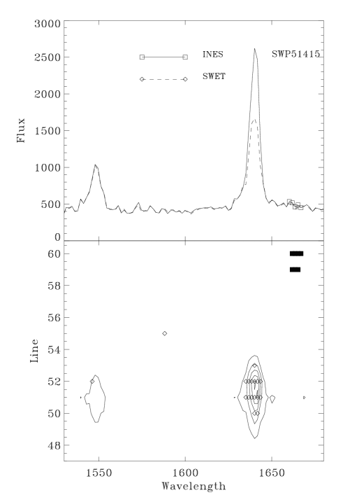
An example of this effect is shown in Figure 7. The spectrum belongs to the symbiotic star AG Dra, characterized by a weak continuum with strong narrow emission lines. The intensity of the HeII 1640Å line given by SWET is approximately half the intensity given by INES. SWET finds part of the emission line outside the extraction profile, consequently flags the pixels as “cosmic rays” (flag -32) and rejects them in the derivation of the final spectrum. It is also worth to note that although half the line is rejected as ”cosmic ray” the flags do not go into the final 1-D quality flag spectrum (see next subsection).

A similar example (a spectrum of Nova Puppis 1991) is shown in Figure 8. The ratio NIV]1486 Å/NIII]1750Å is smaller by a 20% when derived from the SWET spectrum, and clearly in error. These examples demonstrate that SWET results for sources with strong narrow emission lines onto a weak continuum are not optimal and the use of line ratios as diagnostics for physical parameters (temperature, density, chemical abundances …) may be misleading, greatly diminishing the usefulness of the IUEFA for general usage.

Figure 8: In this spectrum of Nova V351 Puppis 1991 none of the emission lines are flagged in either of the extractions, but the NIV] 1486Å and the [NeIV] l602Å lines have been identified by SWET as “cosmic rays”, and their intensity is underestimated. Symbols are as in Figure 7.

2.2.3 Quality flags handling and propagation

Quality flags ($\nu$’s) mark those SILO pixels whose quality is not optimal. The quality of a pixel can be affected by different problems, and there is a gradation in the reliability of the value. Flags are coded in NEWSIPS in such a way that more negative values indicate more important problem conditions.

The importance of a proper handling of $\nu$’s is twofold: firstly, the flags are used to exclude ”bad” pixels during the extraction procedure and secondly, they mark in the final 1-D extracted spectrum those wavelengths where the user should be warned about the reliability of the flux.

Figure 9: This figure is similar to Figure 7, but in this spectrum the HeII line is flagged in the INES spectrum, while it is not in the SWET extraction. As shown in the bottom panel, there are two pixels flagged as saturated in the SILO file. While these flags are propagated to the INES extracted spectrum, they disappear in the SWET extraction. Symbols are as in Figure 7. In particular, the two solid squares on the HeII line in the SILO file mark saturated pixels.

One of the advantages of optimal extraction techniques is that they should be able to recover the flux at flagged pixels as far as the correct cross-dispersion profile is used. However, this ability must be analyzed carefully since flagged pixels are already excluded from the determination of the weighting profile. As an example we will discuss the case of an emission lines spectrum.

In many cases the exposure times were chosen to get a good exposure level in the continuum, frequently resulting in saturation for the the peak of the lines. Then, the core of the strongest lines are flagged as ”Extrapolated ITF” or ”saturated”. If there are only a few pixels flagged it is expected that the correct flux will be obtained from a correct profile. However, the beam pulling effect in IUE images shifts the strong lines with respect to the continuum. Even in the case that the method would be able to reproduce such short scale shifts, if flagged pixels are not used to determine the spatial profile, the weighting profile will be shifted with respect to the actual spatial profile of the line that will be treated as a cosmic ray. For this reason, in the INES extraction only pixels with no real flux information are discarded: reseaux marks, pixels not photometrically corrected, 159DN corrupted pixels and telemetry dropouts.

The way the information about bad quality pixels is passed onto the final 1-D output spectrum is also related to the role these pixels play in the extraction procedure. In the INES extraction, a conservative approach has been followed and the flag of any pixel in the SILO file that makes a contribution to the final 1-D extracted spectrum (i.e. for which the extraction profile is not zero) is passed into the 1-D flag spectrum. This method may propagate flags of pixels whose contribution is almost negligible (e.g. reseaux marks within the aperture, but outside the PSF), but assures that no relevant quality flag is lost. Figure 9 illustrates a case where there are two pixels in the HeII line with the saturation flag in the SILO file. SWET treats the line pixels as a ”cosmic rays” (note the ”-32” flags in SILO file), but neither these flags nor the saturation flags are passed onto the final 1-D spectrum. In contrast, INES reproduces the correct flux and flags the wavelength bins where there are saturated pixels.

2.2.4 Solar contamination removal

By the end of its operational life, the IUE telescope was affected by the so-called FES anomaly (Pérez and Pepoy 1997). In reality, it was not an anomaly of the FES functionality but that name was given because the problem was firstly detected on FES images (Rodríguez-Pascual 1993). For an unknown reason, scattered Sun and Earth light was entering the telescope tube and reaching the on-board detectors (FES and SEC Vidicon cameras). On FES images this light was known as the “streak” because it filled only a portion of the image, producing a pseudo-background. Under the worst conditions the FES detector was fully saturated, providing a number of counts similar to that from a 5th magnitude star. The analysis of the problem showed that light scattered into the telescope was mainly solar in origin (Rodríguez & Fernley 1993). The effect on science images was to contaminate LWP low resolution images with an extended spectrum filling the whole aperture (Fig. 10). SWP images were not affected because of the solar-like spectrum of the scattered light and no measurable contamination has been detected in LWP high resolution spectra. Two types of contamination were identified in LWP images, depending on whether the dominant source was direct sunlight or sunlight reflected on the Earth (Rodríguez-Pascual & Fernley 1993).

Figure 10: Average spatial profile of solar scattered light, based on sky exposures

Figure 11: The thick line shows the average spatial profile from 2900Å to 3300Å in the image LWP28262. The contribution from the solar scattered light contamination and the extraction profile used for the point source are shown as thin lines and the sum of both is represented by crosses. Squares show the extrapolated points of the solar contribution. Note that there is still some remnant contribution of the extended source in the left side of the point source profile.

LWP images contaminated with solar scattered light are identified as extended sources by NEWSIPS. However, the SWET extraction module is forced to perform a point-like source extraction, i.e., restricted to 13 spectral lines, in all LWP images taken after November 1992 and whose IUECLASS does not correspond to solar system objects or sky exposures. This approach does not reduce the solar contribution to the extracted spectrum in a consistent way and definitely does not remove it completely.

Several methods have been evaluated to correct this contamination. The correlation between the strength of the streak as measured with the FES and the strength of the contamination in spectral images led to consider the possibility of building up a spectral template to be scaled by the FES counts. However, this approach was not useful in practice because of the two types of solar spectra found and the large scatter in the FES counts-spectral flux relation (Rodríguez-Pascual & Fernley 1993) associated with the specific light scattering geometry.

The procedure developed in the INES extraction was designed to handle only the most straightforward case: a point-like source, well centered into the aperture. The spectrum of the target does not fill the whole aperture and the solar contamination can be estimated from the spectral lines on both sides of the target PSF. Obviously, this method only works on large aperture spectra; contamination in the small aperture is not corrected.

Figure 12: This figure illustrates how the INES extraction software is able to get rid of most of the solar scattered light contamination. The thick line is the spectrum of the point source, the thin line represents the solar spectrum and the dotted line is a direct boxcar extraction of the whole aperture.

The first step is to identify whether an image is affected by solar contamination. The check is done only on LWP images taken after November 1992 since this was the time its presence was first detected in the FES. The procedure searches for the peak of the average spatial profile. If the contribution of a point source, i.e. up to 11 spectral lines wide, is between 5% and 95% of the total spatial profile then the presence of both an extended and a point-like sources is assumed. This method obviously does not guarantee that the extended source is due to the solar contamination; it may happen that the observation corresponds to a crowded field with several sources. However, we have adopted this approach because any potential user of crowded fields data should already be aware that the IUE Project does not provide individual spectra when several sources are within the aperture. Such spectra need to be individually analyzed from the SILO file. But any user interested in the archival data of an isolated object should not have to worry about contamination by other sources and can take the extracted spectra as the real spectra of the isolated object. Bearing this in mind, it was decided to accept the risk that in some cases the procedure will remove the contribution of an extended component that is not the solar contamination.

Once a LWP image has been identified as contaminated, the 2-D spectrum of the solar light is reconstructed. First, the solar spectrum is extracted as in the standard case, but masking out 11 spectral lines centered at the location of the peak in the average spatial profile. Since sky exposures show that the cross-dispersion profile of the solar contamination is roughly linear in the center of the aperture (Fig. 10), the 2-D spatial profile of the solar contamination within the point-like source location is derived interpolating linearly from the wings of the profile. The 2-D contamination is then reconstructed and subtracted from the SILO file. The point-like spectrum is extracted from the resulting corrected SILO following the standard INES procedures. Spectra in which the correction for solar contamination has been applied are identified by the following message in the FITS header: *** WARNING: SOLAR CONTAMINATION CORRECTION APPLIED

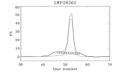
In figures 11 and 12 we show an example of the performance of the method. The average spatial profile in the range 2900-3300Å is shown as a thick line in Fig 11; the thin lines show the profiles estimated for the extended and point sources (crosses represent the sum of both). The squares show the spectral lines discarded to estimate the extended source and later interpolated. The corresponding output spectra are shown in Fig 12.

The performance of this technique has been tested using the data of the blazar PKS 2155-304, extensively monitored with IUE. In particular, two intensive monitoring campaign were carried out in 1991 and 1994 (Pian et al., 1997), before and after the appearance of the FES anomaly. During the 1991 campaign, 98 LWP spectra were obtained. In 1994, IUE was continuously pointing to this target for 10 days starting on May 15th. A total of 236 spectra were obtained, half of them with the LWP camera. Albeit the flux level of the target varied between both runs and even within each run, the effect of the solar scattered light into the LWP camera can be tested because the changes in the spectral shape are small (Pian et al. 1997).

First we compare the ratio of the SWET average spectra of both campaigns (Fig 13). This ratio shows a sharp turn-up beyond 2800Å due to the solar contamination, but the ratio of the INES averages is essentially independent of the wavelength. This is a clear demonstration that SWET is not able to remove the scattered light in the output spectrum. The features beyond 3200Å are typically due to the low S/N in this region of the IUE LWP camera in the individual spectra.

Another test of the presence of solar scattered light in the output spectra is to compare the ratios of fluxes in different wavelength bands. For each campaign and extraction method we have compared the relation between the flux at 2600Å, where no solar contamination is expected and the ratio of the fluxes at 3100Å and 2600Å. This ratio can be taken as a measure of the amount of contamination since the band centered at 3100Å is the most affected. The results are shown in Fig 14. The F(3100Å)/F(2600Å) ratio is definitely larger for the 1994 spectra extracted with SWET. However, the 1991 and 1994 values of this ratio for INES spectra are indistinguisable, although there are still a few data points for which the ratio is larger by $\sim$20%.

Figure 13: Ratio between the average spectra of PKS 2155-304 during the observing campaigns in 1991 and 1994. The thin line is the ratio between SWET spectra and the thick line shows the ratio between INES spectra. Although the 1994 flux is on average 10% lower than in 1991, the index of the power law describing the UV spectrum has not changed noticeably, as indicated by the constant ratio below 2800Å. The sharp rise of the SWET ratio is due to the solar contamination.

Figure 14: The 3100Å region in the SWET extracted spectra of PKS 2155-304 (upper panel) is strongly contaminated by solar scattered light as shown by the ratio F(3100Å)/F(2600Å) in 1994 (squares) and 1991 (crosses). The values of this ratio during 1994 and 1991 are in much better agreement when INES extracted spectra are used (lower panel)

2.3 Homogenization of the wavelength scale

One of the main purposes of the modifications implemented within the INES system is to provide the data in such a form that the user needs to perform the minimum number of operations before starting the scientific analysis and to decrease the instrumental dependence of the extracted spectrum (important for further use by scientist without specific IUE knowledge).

One of the characteristics of the SWET low resolution spectra which, although well documented, can originate some confusion to users, is that the low resolution long wavelength data do not have an uniform wavelength scale, i.e., there are long wavelength spectra with different stepsize and with different number of points in the extracted data. These differences depend on the date of observation and, in the case of the LWR camera, on the ITF used in the processing. The dependency on the date of observation is very small (and it is also present in the SWP camera), but differences between both long wavelength cameras and between both LWR ITFs cannot be neglected. The difference is only in the size of the wavelength step and not in the starting wavelength of the NET spectra (1050 and 1750 Å for short and long wavelength ranges, respectively). Since the Inverse Sensitivity curves are not defined for the full spectral range of the extracted data, LWP and LWR NEWSIPS low resolution calibrated spectra do not start at the same wavelength and have a different number of points.

Any combination or comparison of long wavelength spectra would require the rebinning to a common wavelength scale. In order to facilitate the use of the extracted data, this rebinning has already been built in the INES processing system, assuring homogeneity in the data.

Table 1 summarizes the low resolution wavelength step used in NEWSIPS for each camera.

Table 1: Summary of the wavelength steps of NEWSIPS low resolution spectra

Camera	$\lambda$ step	First calibrated	# of calibrated
	(Å)	pixel	pixels
LWP
pre-1990	2.6627	1851.181	563
post-1990	2.6628	1851.186	563
LWR-ITF A
pre-1980.1	2.6658	1851.300	563
post-1980.1	2.6657	1851.298	563
LWR-ITF B
pre- 1979.9	2.6693	1851.433	562
post- 1979.9	2.6689	1851.418	562
SWP
pre-1990	1.6763	1150.578	495
post-1990	1.6764	1150.584	495

The resampling was performed following this approach:

• All the long wavelength spectra are rebinned to the same wavelength step.

• The size of the new wavelength step is taken as the largest one of all the steps used, i.e. 2.6693 Å per pixel for the LW cameras, and 1.6764 Å per pixel for SWP. The number of calibrated pixels is 495 for the SWP camera, and 562 for the long wavelengths cameras.

• The starting wavelength of the calibrated spectrum has not been modified (i.e. it is the first pixel within the spectral region in which the Inverse Sensitivity Curves are defined).

• Only flux-calibrated points are included in the final spectrum.

• Both the absolute flux and the sigma spectra are rebinned.

• The rebinning of the flux spectrum is made through the following expression:

  $$F_{i}=\frac{\sum_{j}w_{j}f_{j}}{\sum_{j}w_{j}}$$ (4)

  where F_i is the flux of the final rebinned pixel, f_j are the fluxes of the input pixels, and $\omega_{j}$ are the fractions of each original pixel within the new one. It must be noted that for this particular case in which the original and the final wavelength steps are very close to each other, this procedure provides results very similar to a simple linear interpolation.

• The procedure to handle the sigma spectrum is similar, but using the square of the errors instead:

  $$E_{i}=\sqrt{\frac{\sum_{j}w_{j}e^{2}_{j}}{\sum_{j}w_{j}}}$$ (5)

  In this expression, E_i and e_j are the rebinned and original errors, respectively.

• The $\nu$-spectrum is also re-computed. Each final pixel has the minimum (i.e. the “worst”) $\nu$ of the original pixels used in the rebinning. The number of flags in the rebinned spectrum is larger than in the original one, since every pixel contributes to at least two final pixels (e.g. a reseau mark originally flagged in two consecutive pixels would result in three flagged points in the resampled spectrum).

  It must be noted that the largest increase in the size of wavelength step (which corresponds to the LWP camera) is by a 0.25%. The spectral resolution for this camera is 5.2Å(1.95 pixels, Garhart et al. 1997). Consequently this rebinning does not introduce any significant degradation in spectral resolution.

3 INES Data quality evaluation

3.1 Flux repeatability

The repeatability of the INES low resolution spectra has been tested on a large sample of spectra of some of the IUE standard stars. The only restriction imposed has been to include only non–saturated spectra of similar level of exposure (i.e. similar exposure times) in order to avoid the remaining non–linearity effects (see Section 3.3). The spectra cover all the range of observing epochs and camera temperatures. Therefore it must be taken into account that the repeatability, as defined here, includes implicitly the uncertainties in the camera time degradation and the temperature corrections.

The study has been performed in 100 Å wide bands. Table 2 lists the central wavelength of the bands and the repeatability, defined as the percent rms respect to the mean intensity of the band. The figures in brackets are the number of spectra considered in each case.

Table 2: Flux repeatability of INES low resolution spectra

SWP

	BD+28 4211	BD+75 325	HD 60753	Average
Band	(292)	(196)	(228)
1200	3.82	3.11	5.29	4.07
1300	3.12	2.50	3.08	2.90
1400	1.99	1.95	2.09	2.01
1500	1.84	1.70	1.90	1.81
1600	2.00	1.86	2.10	2.04
1700	2.21	1.68	1.99	1.96
1800	2.03	1.74	1.97	1.91
1900	2.10	2.03	1.94	2.02

LWP

	BD+28 4211	BD+75 325	HD 60753	Average
Band	(232)	(223)	(225)
1900	18.21	16.90	15.69	16.93
2000	3.43	3.65	4.75	3.94
2100	4.19	3.81	4.61	4.20
2200	3.11	3.29	4.83	3.74
2300	3.54	3.59	4.49	3.87
2400	2.78	2.71	3.19	2.89
2500	2.35	2.38	2.63	2.45
2600	2.21	2.17	2.64	2.34
2700	1.99	2.13	2.27	2.23
2800	1.94	2.07	2.06	2.02
2900	1.94	2.26	2.06	2.09
3000	2.42	2.71	2.24	2.46
3100	4.00	4.12	3.51	3.88
3200	7.77	6.93	5.64	6.78
3300	14.90	16.84	11.29	14.34

LWR

	BD+28 4211	BD+75 325	HD 60753	Average
Band	(89)	(86)	(76)
1900	7.77	7.14	7.92	7.61
2000	4.51	4.99	5.66	5.05
2100	3.84	4.25	5.26	4.45
2200	4.07	4.72	5.50	4.76
2300	3.71	3.64	4.57	3.97
2400	3.43	3.48	4.24	3.72
2500	2.92	3.00	3.19	3.04
2600	3.05	2.94	3.55	3.18
2700	3.20	3.18	3.95	3.44
2800	3.42	3.66	3.66	3.58
2900	3.67	3.77	3.77	3.74
3000	4.31	3.19	4.17	3.89
3100	5.18	4.28	4.62	5.69
3200	10.19	9.18	10.22	9.86
3300	50.35	41.19	54.17	48.57

As expected, the best repeatability is attained in the regions of maximum sensitivity of the cameras. In the SWP the repeatability is around 2% longward 1400 Å. For the LWP camera, values lower than 3% are reached in the central part of the camera, 2400-3000 Å. At the extreme wavelengths the repeatability is around 15%. The results are slightly worse for LWR most likely due to the instability of the camera after it ceased to be used for routine operations. The repeatability is between 3-4% in the region 2300-3000 Å. Particularly bad is the 3300 Å band, but at the shortest wavelengths (1850-1950 Å) the repeatability is substantially better than in the LWP camera. When considering only images taken when LWR was the prime long wavelength camera, the repeatability is similar to that of LWP in the central part of the camera.

3.2 Reliability of extraction errors

Figure 15: Comparison of the extraction errors (Errors) in INES with the dispersion around the mean spectrum (STD) for three standard stars, after correction with the coefficients shown in Table 3 for the SWP camera.

Figure 16: Same as Figure 15, but for the LWP camera

In addition to the flux spectrum, optimal extraction methods also provide an error spectrum. Formally, these errors only account for the uncertainties in the extraction procedure, based on the noise model of the detector. They do not include uncertainties driven by parameters affecting the image registration. During the processing, corrections are applied to account for the changes in temperature in the head amplifier of the cameras (THDA) and the loss of sensitivity of the detectors. All these corrections have their own uncertainties. There are yet other systematic errors that affect the absolute fluxes, as the uncertainty in the inverse sensitivity curve, but do not affect the comparison of different sets of IUE spectra. The extraction errors can be used to compare fluxes in different bands of the same spectrum or to compute weighted averages of a set of spectra, but they may not be appropriate to evaluate the variability of a source or an spectral feature, due to the considerations given above.

Figure 17: Same as Figure 15, but for the LWR camera with a voltage of -5.0 kV.

In order to check the statistical validity of the errors provided by the INES extraction, we have taken the same data set used in the previous section (i.e. a large sample of spectra of standard stars with similar level of exposure) and compared the rms around the mean with the average errors as given by the extraction procedure. In general, the extraction errors underestimate the errors represented by the rms in the three cameras, with the exception of the shortest wavelength end of the LWP camera. In the SWP camera the errors are underestimated by $\sim$20-40% , depending on the wavelength. In the LWR the ratio between extraction and actual errors is nearly constant (12%) all along the camera, while in the LWP the discrepancy can be as large as 40% at the longest wavelength. In this camera, shortward 2400Å the extractions errors are too large by 15–20%. This region is very noisy and there are reasons to suspect that such a noise departs significantly from a gaussian behaviour.

It is also found that the dependency of the ratio STD/Error (where “STD” is the standard deviation around the mean spectrum, and “Error” is derived from the extraction errors) with wavelength can be well represented by a straight line with the coefficients shown in Table 3. Reliable values for these coefficients could not be obtained for the LWR camera operated at -4.5kV due to the scarcity of data.

Table 3:

Camera	a	b
LWP	-0.49	6.2$\times 10^{-4}$
SWP	1.11	1.6$\times 10^{-4}$
LWR(-5.0kV)	1.12	-3.1$\times 10^{-6}$

In order to compare fluxes in different spectra of the same object, the extraction errors must be modified according to

$$\varepsilon(\lambda)=a+b\varepsilon_{{\rm E}}(\lambda)$$ (6)

where $a$ and $b$ are the coefficients in Table 3 and $\varepsilon_{{\rm E}}(\lambda)$ are the extraction errors.

The results of the application of this correction are shown in figures 15, 16 and 17. The dispersion around the expected value of 1 is 0.15 for SWP, 0.17 for LWP and 0.18 for LWR. The structure still seen in these figures might be related to remaining non linearities in the ITF’s (see below).

3.3 Flux Linearity

Despite the correction applied during the processing of the IUE data through the application of the Intensity Transfer Functions (ITFs), the final spectra are still affected by non-linearities to some degree. As a consequence, spectra of the same non-variable object observed with different exposure times might have slightly different flux levels.

Figure 18: Ratios of different exposure levels to the 100% for the three cameras. The thick horizontal line marks the saturated part in the overexposed spectra

Table 4: Linearity properties of INES low resolution spectra (ratios to 100% exposure)

SWP

Band	8%	19%	28%	39%	59%	79%	121%	151%
1200	0.78	0.87	0.88	0.86	0.92	0.98	1.04	1.14
1300	0.81	0.90	0.87	0.92	0.96	0.99	1.03	1.04
1400	0.92	0.96	0.95	0.96	0.96	1.01	1.02	1.03
1500	0.88	0.93	0.93	0.95	0.96	0.98	0.99	0.98
1600	0.92	0.97	0.96	0.95	0.98	1.01	1.02	1.00
1700	0.83	0.99	0.97	0.97	1.00	1.02	1.03	1.00
1800	0.98	1.00	0.97	1.00	1.00	1.03	1.01	1.02
1900	0.96	0.94	0.95	0.97	1.00	1.03	1.03	1.02

LWP

Band	19%	39%	59%	79%	129%	150%	200%
1900	1.33	1.28	1.04	1.11	1.03	1.03	1.01
2000	1.10	1.01	1.01	1.00	1.02	1.03	1.00
2100	1.06	1.04	1.03	1.04	1.02	1.01	1.04
2200	0.97	1.02	0.99	1.03	1.02	1.01	1.06
2300	0.97	0.98	1.00	1.00	1.02	0.99	1.01
2400	1.05	1.00	1.03	1.03	1.04	1.03	1.05
2500	1.04	1.05	0.99	0.99	1.00	1.01	1.07
2600	0.94	0.96	0.96	0.99	1.00	1.01	1.09
2700	0.95	0.96	0.99	0.99	1.02	1.05	1.12
2800	1.00	0.99	1.02	1.00	1.03	1.03	1.11
2900	1.08	1.04	1.05	1.02	1.05	1.05	1.08
3000	1.02	1.00	1.02	1.03	1.05	1.03	1.05
3100	0.93	0.99	0.95	1.01	1.07	1.05	1.02
3200	1.13	0.86	0.95	1.05	1.10	0.97	1.07
3300	1.02	1.16	1.30	1.29	1.11	1.37	1.12

LWR-ITF-B

Band	32%	56%	167%	251%
1900	0.94	1.06	1.09	1.09
2000	0.94	1.01	1.01	1.02
2100	1.05	1.05	1.02	1.05
2200	1.01	1.00	1.02	1.02
2300	0.93	0.97	1.01	1.02
2400	1.03	0.97	1.01	1.03
2500	0.98	1.00	1.02	1.01
2600	0.97	0.98	1.02	0.90
2700	0.94	0.93	1.00	0.87
2800	0.93	0.99	1.02	0.92
2900	0.95	1.00	1.00	1.02
3000	0.99	0.95	1.01	1.05
3100	0.98	0.99	0.98	0.99
3200	1.16	1.08	1.01	1.01
3300	1.63	1.29	1.06	1.15

In order to evaluate the importance of the remaining non-linearities we have chosen, for each camera, a set of low resolution spectra of the standard star BD+28 4211, extracted with the INES system, obtained close in time under similar temperature conditions and with different exposure times. In each set one of the spectra is defined as a 100% exposure, and all the other are referred to that one.

The summary of the data used for each camera is as follows:

• SWP: Nine spectra taken in December 1993, with exposure times ranging from 2 sec (9%) to 40 sec (150%).

• LWP: Nine spectra taken in October 1986, with exposure times ranging from 10 sec (20%) to 100 sec (200%).

• LWR: Five spectra taken in August 1980, with exposure times ranging from 20 sec (30%) to 150 sec (250%). All this spectra have been processed with ITF–B (Garhart et al. 1997), which is the one giving the best correlation coefficient in this case, as in most of the pre-1984 LWR spectra.

Each spectrum was binned into in 100 Å bands and divided by the corresponding reference exposure. The results are summarized in Table 4. Examples of the behaviour of different spectral bands for each of the cameras as a function of the level of exposure are shown in Figure 18.

In the SWP camera the largest departures from linearity are found at the short wavelength end of the underexposed spectra, where flux can be underestimated by up to a 20%. Apart from this case, longward Lyman $\alpha$ ratios to the 100% spectrum are generally within$\pm$5%. The best results are achieved in the 1800 Å band, where linearity is within $\pm$ 3%.

For the LWP camera the largest non-linearities occur at the extreme wavelengths (1900, 3300 Å), where the flux is largely overestimated. Except for these bands, linearity is within $\pm$ 5% for spectra with exposure levels from 40% to 150%. In the saturated region of the most exposed spectrum the flux is overestimated by 10%. Excluding the saturated region, the bands which show the best linearity characteristics (within $\pm$ 3%) are those centered at 2800 and 3000 Å.

The LWR camera shows the largest non-linearities at the longest wavelengths of the underexposed spectra. Linearity remains within $\pm$ 5% for exposure levels above 60%. The most linear bands are those centered at 2500, 2900 and 3100 Å. In the saturated part of the 200% spectrum, the flux is underestimated by approximately 10%. However, the flux is correct in the 170% spectrum, which is also saturated.

4 Summary

Within the framework of the development of the ESA INES Data Distribution System foe the IUE Final Archive, IUE Low Dispersion spectra have been re-extracted from the bi-dimensional SILO files with a new extraction software. INES implements a number of major modifications with respect to the SWET extraction applied to the early version of the IUE Final Archive. The improvements in INES deal with the noise model, the optimal extraction method, the homogenization of the wavelength scale and the flagging of the absolute calibrated extracted spectra.

• The noise models for the different cameras have been re-derived to correct anomalies at high and low exposure levels in those used in SWET. The noise model results in a considerably more realistic estimate of the actual extraction errors in the IUE spectra.

• The algorithms to compute the camera background and the extraction profile are more consistent with the nature of the IUE detectors and result in a significantly improved data quality.

• Weak extended or miscentered spectra are more adequately handled. The fluxes of strong emission lines in weak continuum spectra are more reliable and consistent in the INES extraction.

• The handling and propagation of quality flags to the final extracted spectra has been improved. This implies a larger number of pixels flagged, but also a more correct information for the user of potential problems in the data.

• A major improvement has been reached in the removal of the solar contamination in LWP images after 1992.

• In order to facilitate an easier use of the data, all the spectra of a given range (short and long) have been resampled to a common wavelength scale.

As a general rule, INES data are similar or superior to SWET. Although the INES spectra may at times give somewhat lower signal-to-noise ratio than those obtained through SWET (e.g. when boxcar extraction is required to maintain data validity), the INES extraction results in a higher reliability of the IUEFA data, allowing direct intercomparison of all low resolution spectra, through an adequate treatment of errors, flags and warning messages in the image header.