Characterizing the structure of interstellar turbulence

Abstract

Modeling the structure of molecular clouds depends upon good methods to statistically compare simulations with observations in order to constrain the models. Here we characterize a suite of hydrodynamical and magnetohydrodynamical (MHD) simulations of supersonic turbulence using an averaged wavelet transform, the $\Delta$-variance, that has been successfully used to characterize observations. We find that, independent of numerical resolution and dissipation, the only models that produce scale-free, power-law $\Delta$-variance spectra are those with hypersonic rms Mach numbers, above $M\sim 4$, while slower supersonic turbulence tend to show characteristic scales and produce non-power-law spectra. Magnetic fields have only a minor influence on this tendency, though they tend to reduce the scale-free nature of the turbulence, and increase the transfer of energy from large to small scales. The evolution of the characteristic length scale seen in supersonic turbulence follows exactly the $t^{1/2}$ power-law predicted from recent studies of the kinetic energy decay rate.

1 Introduction

Although numerical simulations of transsonic and supersonic turbulence appropriate to interstellar gas have been carried out for several years now (Porter, Pouquet, & Woodward 1992, 1994; Padoan & Nordlund 1999; Mac Low et al. 1998; Stone, Ostriker, & Gammie 1998) there are only a few direct comparisons between numerical results and astrophysical observations (e.g. Falgarone et al. 1994; Padoan et al 1999; Rosolowsky et al. 1999). This is mainly due to the lack of appropriate measures applicable both to simulated and observed structures. Measures common for turbulence studies like the power spectrum of spatial or velocity fluctuations or the probability distribution of velocity increments are not easily applied to observations where their use is greatly impaired by the limitations due to finite signal to noise ratio and limited telescope resolution.

To obtain clues to the true physical nature of interstellar turbulence, characteristic scales and any inherent scaling laws have to be measured and modelled. A major problem with characterizing both the observations and the models is to determine what scaling behaviour, if any, is present in complex turbulent structures. Both the velocity and density fields need to be considered, but only the radial velocity and column densities can be observed.

One measure useful for characterizing structure and scaling in observed maps of molecular clouds is the $\Delta$-variance, $\sigma^{2}_{\Delta}$, introduced by Stutzki et al. (1998). It can better separate observational effects from the real cloud structure than e.g. the power spectrum or fractal dimensions. The $\Delta$-variance spectrum clearly shows characteristic scales and scaling relations, and its logarithmic slope can be analytically related to the spectral index of the corresponding power spectrum.

Stutzki et al. (1998) and Bensch et al. (1999) have applied the $\Delta$-variance analysis to observations of the Polaris Flare and the FCRAO survey of the outer galaxy. They found a relatively universal law describing these clouds, with a power law structure at scales below the cloud size and the general cloud size as the only characteristic scale within the resolution limit. Given the limited number of samples, however, it is not yet possible to draw conclusions on the scaling of turbulence in molecular clouds in general. To study the common behaviour and differences between several clouds and interstellar regions the analysis of more and larger maps obtained with a good signal-to-noise ratio is required.

In order to understand the physical significance of the characterization of the observational maps by $\Delta$-variance spectra, we apply here the same analysis to simulated gas distributions resulting from MHD models. In this first paper, we try to get a general feeling for the scaling behaviour in different models, and for the influence of the different parameters and numerical approaches on the produced structures. We only perform a qualitative comparison to the observations here. In a subsequent paper we will attempt to make a detailed fit of several observed regions using MHD models including the solution of the radiative transfer problem.

2 Structure measure by the $\Delta$-variance

2.1 Definitions

The $\Delta$-variance was comprehensively introduced by Stutzki et al. (1998). We will repeat here only the formalism essential for the further analysis in this paper.

The $\Delta$-variance is a type of averaged wavelet transform that measures the variance in an $E$-dimensional structure $f(\@vec{r})$ filtered by a spherically symmetric down-up-down function of varying size (Zielinsky & Stutzki 1999). It is defined by

$$\sigma_{\Delta}^{2}(l)=\int_{-\infty}^{\infty}\left((f(\@vec{r})-\langle f\rangle)*{\bigodot}_{l}(\@vec{r})\right)^{2}d\@vec{r}$$ (1)

where, the $*$ stands for a convolution and $\bigodot_{l}$ describes the down-up-down function with the length $l$ of each step

$${\bigodot}_{l}(\@vec{r})={\cal V}_{E}^{-1}({2\over l})^{E}\left\{\begin{array}[]{ll}1&|\@vec{r}|\leq l/2\\ -1/(3^{E}-1)&l/2<|\@vec{r}|<3l/2\\ 0&|\@vec{r}|>3l/2\end{array}\right.$$ (2)

with ${\cal V}_{E}$ being the volume of the $E$-dimensional unit sphere.

Thus, the $\Delta$-variance measures the amount of structural variation on a certain scale, e.g. in a map or three-dimensional distribution. A familiar, slightly different kind of variance defined for one-dimensional problems is the Allan-variance commonly used for stability investigation (Schieder et al. (1989)). In contrast to the $\Delta$-variance, it works with a non-symmetric up-down filter.

Instead of convolving the structure in ordinary space with a filter function one can carry out the $\Delta$-variance analysis in Fourier space by simple multiplication. This directly relates the $\Delta$-variance to the power spectrum of a structure. If $P(k)$ is the radially averaged power spectrum of the structure $f(\@vec{r})$, the $\Delta$-variance is given by

$$\sigma_{\Delta}^{2}(l)=\int_{0}^{\infty}P(k)\;|\tilde{\bigodot}_{l}(k)|^{2}k^{E-1}dk$$ (3)

where $\tilde{\bigodot}_{l}$ is the Fourier transform of the $E$-dimensional down-up-down function with the scale length $l$, and we are using $k$ to denote the spatial frequency or wavenumber.

If the power spectrum is given by a simple power law, $P(k)\propto k^{-\zeta}$, the $\Delta$-variance also follows a power law $\sigma_{\Delta}^{2}\propto l^{\alpha}$ with $\alpha={\zeta-E}$ within the exponential range $0\leq\zeta<E+4$. (To avoid confusion with the ratio between thermal and magnetic pressure we use $\zeta$ for the power spectral index rather than the variable $\beta$ used by Stutzki et al. (1998) and Bensch et al. (1999).) The main advantages of the $\Delta$-variance compared to the direct computation of the Fourier power spectrum are the clear spatial separation of different effects influencing observed structures like noise or finite observational resolution, and the robustness against singular variations due to the regular filter function.

Furthermore, for most astrophysical structures, where a periodic continuation is not possible, Bensch et al. (1999) has shown that the periodicity artificially introduced by the Fourier transform can lead to considerable errors. Here, even the $\Delta$-variance has to be determined in ordinary space. For the simulations examined in this paper, periodic wrap around is not a problem because it is already explicitly assumed, so we apply the faster Fourier method to determine their $\Delta$-variance spectra.

Figure 1: Comparison of 3D $\Delta$-variance spectra to Fourier power spectra for $128^{3}$ models of turbulence driven at wavenumbers of $k_{d}=2$ (solid), $k_{d}=4$ (dotted), and $k_{d}=8$ (dashed), demonstrating that the analytic relation between power spectrum slope and $\Delta$-variance spectrum slope also holds for the local behavior of structures not showing a straight power-law.

In Fig. 1 we compare the power spectrum and $\Delta$-variance for three simulations described below. They have different driving scales, and therefore each shows a different characteristic scale visible as a turn-over at large lags in the $\Delta$-variances and at small wavenumbers in the power spectrum, respectively. At smaller lags and higher wavenumbers power laws can be seen in both cases (with their slopes related by the analytic relation given above). A steep drop-off follows at the smallest scales indicating the resolution limit of the simulation. The power laws are equivalent in both cases, but the characteristic scale at one end and the resolution limit at the other end of the spectrum can be more clearly seen in the $\Delta$-variance. The smooth spatial filter function in the $\Delta$-variance analysis still provides a good measure for the behavior at large scales whereas the power spectrum suffers from the low significance of the few remaining points there.

The $\Delta$-variance analysis of astronomical maps was extensively discussed and demonstrated by Bensch et al. (1999). In all the observations analyzed by them, the total cloud size was the only characteristic scale detected by means of the $\Delta$-variance. Below that size they found a self-similar scaling behaviour reflected by a power law with index $\alpha=0.5\dots 1.3$ corresponding to a Fourier power spectral index $\zeta=2.5\dots 3.3$. The analysis of further maps will be discussed in future work.

2.2 Two-dimensional maps and three-dimensional structures

In the application to molecular cloud structure simulations we have to restrict the analysis either to the three-dimensional structure or to the two-dimensional projection of the structure which would be astronomically observed, e.g. in optically thin lines or the FIR dust emission.

Stutzki et al. (1998) have shown that the spectral index of the power spectrum $\zeta$ for an spatially isotropic structure remains constant on projection. This means that the projected map of three-dimensional density structures shows the same $\zeta$ as the original structure as long as we assume that the astronomical structure is on the average isotropic. Consequently the slope of the $\Delta$-variance grows by 1 in projection.

Figure 2: Demonstration of the equivalence of 2D projected and properly transformed 3D $\Delta$-variance spectra. Projected $\Delta$-variances spectrum of a model density cube (model C from Mac Low et al. 1998 at $t=0.1t_{s}$, where $t_{s}=L/c_{s}$ is the sound-crossing time) are shown. The dotted line is the corresponding three-dimensional $\Delta$-variance multiplied by the local lag. The solid line is additionally shifted by a factor $\pi/4$ to correct for the average length reduction on projection.

In Fig. 2 we demonstrate this for a simulation where we determined the $\Delta$-variance of the three-dimensional structure and the $\Delta$-variances of the three perpendicular projections. The dashed lines show the three projected $\Delta$-variances. Now we multiply the three-dimensional $\Delta$-variance by the abscissa values to obtain the same local slope as measured in two dimensions (dotted line). However, we still have to correct for the scale length of the measure. The length of an arbitrary three-dimensional vector is reduced on projection to two dimensions by a factor $\pi/4$ on the average. Therefore, we adjust the local scale by this factor for the $\Delta$-variance determined in three dimensional space. The resulting plot is shown as the thick solid line in Fig. 2. We obtain exactly the same general behaviour as for the projected maps. The equivalent plot for numerous other models verified this as a general behavior. Hence, we can either consider the three-dimensional variance or the projected variances and can simply translate them into each other.

The treatment of the three-dimensional variances is favourable from the viewpoint that it measures exactly the scales as they occur in the density structure. However, the projected maps are favourable to have a means of direct comparison to astronomical observations. Putting the relation to the observations at first priority, we will show in the following the variances translated to the two-dimensional behaviour and we will only mention the physical three-dimensional scales if they appear to be especially prominent.

In this paper, we will restrict ourselves to simple projections taking them as representations of the integrated map of optically thin lines or optically thin continuum emission. We will not treat the full radiative transfer problem which had to be solved for a general treatment. Optical depths effects in fractal and random structures were discussed by Ossenkopf et al. (1998) and they will be taken into account in a subsequent paper dealing with the simulation of certain molecular clouds.

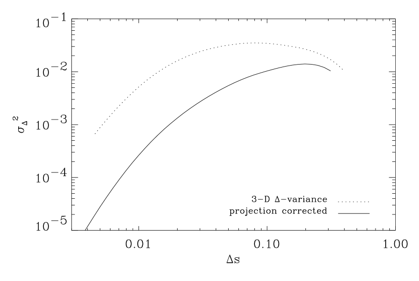
Figure 3: $\Delta$-variance of a decaying hydrodynamic model determined in 3-D and rescaled for projection effects as if it were measured as a 2-D map.

As a side-result of this comparison we find however, that the treatment of maps instead of three-dimensional cubes by observers can easily lead to a misinterpretation of the structure scaling. Fig. 3 compares the three-dimensional $\Delta$-variances computed in 3-D and the same variance corrected for 2-D projection as it could be measured by an observer for a hydrodynamic decaying turbulence model. Whereas the plot for 3-D only shows a broad distribution of structures, the human eye tries to see in the 2-D curve at least a reasonable range with a power law between 0.03 and 0.2. Except for the smallest lags dominated by numeric viscosity as discussed below the plot is quite similar to variances obtained e.g. by Stutzki et al. (1998) for molecular clouds. Hence, noncritical observers might be forced to see a self-similar behaviour even if there is no strong indication for a power law.

3 Numerics

3.1 Computations

We use simulations of uniform decaying and driven turbulence with and without magnetic fields described by Mac Low et al. (1998) in the decaying case and by Mac Low (1998) in the driven case. These simulations were performed with the astrophysical MHD code ZEUS-3D (Clarke 1994). This is a three-dimensional version of the code described by Stone & Norman (1992a, b) using second-order advection (Van Leer 1977), that evolves magnetic fields using constrained transport (Evans & Hawley 1988), modified by upwinding along shear Alfvén characteristics (Hawley & Stone 1995). The code uses a von Neumann artificial viscosity to spread shocks out to thicknesses of three or four zones in order to prevent numerical instability, but contains no other explicit dissipation or resistivity. Structures with sizes close to the grid resolution are subject to the usual numerical dissipation, however.

In this paper, we attempt to use these simulations to derive some of the observable properties of supersonic turbulence. Although our dissipation is clearly greater than the physical value, we can still derive useful results for structure in the flow that does not depend strongly on the details of the behavior at the dissipation scale. Such structure exists in incompressible hydrodynamic turbulence (e.g. Lesieur 1997). In Mac Low et al. (1998) it was shown that the energy decay rate of decaying supersonic hydrodynamic and MHD turbulence was independent of resolution with a resolution study on grids ranging from $32^{3}$ to $256^{3}$ zones. Because both numerical dissipation and artificial viscosity act across a fixed number of zones, increasing resolution yields decreasing dissipation. The results we describe in this paper suggest that in some cases observable features may be independent enough of resolution, and thus of the strength of dissipation. Despite the limitations of our method we can therefore draw quantitative conclusions. Again, we support this assertion by appealing to resolution studies whenever possible.

The simulations used here were performed on a three-dimensional, uniform, Cartesian grid with side $L=2$, extending from -1 to 1 with periodic boundary conditions in every direction. For convenience, we have normalized the size of the cube to unity in the analyses described here, so that all length scales are in fractions of the cube size. An isothermal equation of state was used in the computations, with sound speed chosen to be $c_{s}=0.1$ in arbitrary units. The initial density and, in relevant cases, magnetic field were both initialized uniformly on the grid, with the initial density $\rho_{0}=1$ and the initial field parallel to the $z$-axis.

The turbulent flow is initialized with velocity perturbations drawn from a Gaussian random field determined by its power distribution in Fourier space, following the usual procedure. As discussed in detail in Mac Low et al. (1998), it is reasonable to initialize the decaying turbulence runs with a flat spectrum with power from $k_{d}=1$ to $k_{d}=8$ because that will decay quickly to a turbulent state. Note that the dimensionless wavenumber $k_{d}=L/\lambda_{d}$ counts the number of driving wavelengths $\lambda_{d}$ in the box. A fixed pattern of Gaussian fluctuations drawn from a field with power only in a narrow band of wavenumbers around some value $k_{d}$ offers a very simple approximation to driving by mechanisms that act on that scale. To drive the turbulence, this fixed pattern was normalized to produce a set of perturbations $\delta\@vec{\nu}(x,y,z)$, and at every time step add a velocity field $\delta\@vec{v}(x,y,z)=A\delta\@vec{\nu}$ to the velocity $\@vec{v}$, with the amplitude $A$ now chosen to maintain constant kinetic energy input rate, as described by Mac Low (1998).

3.2 Resolution Studies

In Figure 4 we show how numerical resolution, or equivalently the scale of dissipation, influences the $\Delta$-variance spectrum that we find from our simulations. We test the influence of the numerical resolution on the structure by comparing a simple hydrodynamic problem of decaying turbulence computed at resolutions from $64^{3}$ to $256^{3}$, with an initial rms Mach number $M=5$ (Model D from Mac Low et al. 1998).

Figure 4: $\Delta$-variance of the density cubes (translated to two-dimensions) for a model of decaying hydrodynamic turbulence at a time $t/t_{s}=0.1$, computed using numerical resolutions of $64^{3}$, $128^{3}$, and $256^{3}$.

In contrast to the results from Mac Low (1999) which showed little dependence of the energy dissipation rate on the numerical resolution, we find here remarkable differences in the scaling behaviour of the turbulent structures. At small scales we find a very similar decay in the relative structure variations up to scales of about 10 times the pixel size (0.03, 0.06, and 0.1 for the resolutions $256^{3}$, $128^{3}$, and $64^{3}$, respectively) in all three models. This constant length range starting from the pixel scale clearly identifies this decay as an artifact from the simulations which can be attributed to the numerical viscosity acting at the smallest available size scale.

Another very similar behaviour can be observed at the largest lags where the relative structure variations decay for all three simulations on a length scale covering a factor two below half the cube size. This structure reflects the original driving of the turbulence with a maximum wavenumber $k_{d}=8$ that manifests itself in the production of structure on the corresponding length scale. Only for the $256^{3}$ cubes we find a range of an approximately self-similar behaviour at intermediate scales that is not yet smoothed out by the influence of numerical viscosity.

Structures larger than at most half the cube size are suppressed by the use of periodicity in the simulations. Together with the viscosity range of about 10 pixels there is only a scale factor about 10, 5 or 3 remaining for the three different resolutions where we can study true structure not influenced by the limiting conditions of the numerical treatment. For the derivation of reliable scaling laws, we must therefore use at least simulations on the $256^{3}$ grid. On the other hand we know, however, that the limits of the observations also constrain the scaling factor for structure investigations in observed maps to at most a factor 10 in general (Bensch et al. (1999)).

Although we have plotted here only the results for a hydrodynamic model there are no essential differences to the resolution dependence when magnetic fields are included as discussed below.

3.3 Statistical Variations

Another question concerns the statistical significance of the structure in the simulations. Since each simulation and even each time step provides another structure there is a priori no reason to believe that a statistical measure like the $\Delta$-variance is about the same for each realization of a given HD/MHD problem.

Restricted by the huge demand for computing power in each simulation we cannot provide a statistically significant analysis of many realizations for each problem. However, we will try to provide some general clues for the uncertainty of the $\Delta$-variance measured for a certain structure.

A first impression can be obtained from the differences in the three projections of one cube in Fig. 2. Because each projection provides an independent view on the three-dimensional structure their variation can be considered a rough measure for the statistical significance of the $\Delta$-variance plots. We see that the curves agree well up to lags of about a quarter of the cube size but deviate considerably at larger lags. This is explained by the number of structures contributing to the variations at each scale. Whereas we find many small fluctuations dominating the variance at small scales there is in general only one main structure responsible for the variance at the largest scale. Its different appearance from different directions then produces the uncertainty in the $\Delta$-variance there.

Looking at the variance determined in three dimensions in Fig. 2 we see however that it provides already a kind of average over the three projected functions. Analyzing the three-dimensional cubes thus removes already part of the statistical variations that could be seen by an observer when looking at the two-dimensional projections only. The statistical uncertainty is reduced for the $\Delta$-variances determined in three dimensions considered below.

As another estimate for the uncertainty in this case we study the variances for different time steps in the evolution of a continuously driven hydrodynamic model. In the evolution of the simulation different structures are produced which should behave statistically equal since the general process of their formation and destruction remains the same.

Figure 5: Different time steps in the evolution of a driven model (model HE2 from Mac Low 1999 with $k_{d}=2$ driving) which should remain statistically stationary, showing that the $\Delta$-variation spectra don’t vary much due to turbulent evolution. The first time is $0.4t_{s}$, and succeeding plots are separated by times of $0.05t_{s}$, or 0.75 the crossing time at the rms velocity.

Fig. 5 shows four different timesteps in an HD model driven at wavenumber $k_{d}=2$ each separated by 0.75 the box crossing time at the rms velocity. The variations even at larger scales are much less than in Fig. 2. It appears that the $\Delta$-variance does a good job of characterizing invariant properties of the structure. Only for high accuracy determinations of the slope or the reliable identification of self-similarity ensemble averages should be taken by computing many realizations.

4 Results

4.1 Decaying hydrodynamic turbulence

We have computed the $\Delta$-variance spectra for two models of decaying hydrodynamic turbulence, one with initial rms Mach number $M=5$, noted as Model D in Mac Low et al. (1998), and one otherwise identical model with initial $M=50$, not published before. As noted above, these models were excited with a flat-spectrum pattern of velocity perturbations, which would correspond to a rather steep spectrum $\sigma_{\Delta}^{2}\propto L^{-2}$ in 2D or $\propto L^{-3}$ in 3D, respectively. Both were run at a resolution of $256^{3}$.

Figure 6: Time sequence of decaying turbulence originally driven by M=5 (upper plot, model D from Mac Low et al. 1998), and M=50 (lower plot), at times in units of the sound crossing time $t_{s}$.

The first time steps in Figure 6 show that only hypersonic turbulence provides a self-similar behavior, indicated by a power-law $\Delta$-variance spectrum. In this case, there appears to be structure corresponding to a power-law spectrum of $k^{-2.5}$, somewhat steeper than the $k^{-2}$ that would be expected from a simple box full of step-function shocks, but approaching the steepness observed for real interstellar clouds. When the turbulence decays to supersonic rms velocities at later times, or in the model having only supersonic initial velocities, the spectrum indicates no self-similar structure but a distinctive physical scale that evolves with time to larger sizes.

We speculate that a physical explanation for this observation might be drawn from the nature of dissipation in supersonic turbulence. Energy does not cascade from scale to scale in a smooth flow through wavenumber space as is assumed by analyses following Kolmogorov (1941) for subsonic turbulence. Rather, energy on large scales is directly transferred to scales of the shock thickness by shock fronts, and there dissipated. As a result, energy is not added to small and intermediate scale structures at the same rate that it is dissipated. Combined with a fairly steep power spectrum, this means that the smaller scale structures will be lost to viscous dissipation first, moving the typical size to larger and larger scales.

We can quantify the change in typical scale by simply fitting a power-law to the lag $L_{pk}$ at which $\sigma_{\Delta}^{2}$ reaches a peak. This was done for the 3D $\Delta$-variance where the peak appears more prominent than in Fig. 6 and represents the true length scale without projection effects. For the model starting at Mach 5 we find a variation in time of $L_{pk}\propto t^{q}$ with $q=0.51$.

These decaying turbulence models were found by Mac Low et al. (1998) to lose kinetic energy at a rate $E_{\rm kin}\propto t^{-\eta}$, with $\eta\simeq 1$. However, Mac Low (1999) showed that driven hydrodynamic turbulence dissipates energy $E_{\rm kin}\propto v^{3}/\ell$, corresponding to a kinetic energy decay rate of $\eta=2$ if the effective decay length scale $\ell$ were independent of time. From this observation, a time dependence of $\ell\propto t^{1/2}$ was deduced. Mac Low (1999) also showed that the characteristic driving length-scale $1/k_{d}$ was the most likely identification for $\ell$. Identifying $\ell$ for decaying turbulence with the length scale containing the most power in the $\Delta$-variance spectrum $L_{pk}$ seems natural, and yields excellent agreement in the time-dependent behavior of the length scale, since $L_{pk}\propto t^{0.51}$.

4.2 Driven hydrodynamic turbulence

In Figure 7 we show the $\Delta$-variance spectra for models of supersonic hydrodynamic turbulence driven with a fixed pattern of Gaussian random perturbations having only a narrow range of wavelengths and two different energy input rates. The driving wavelengths are 1/2, 1/4, and 1/8 of the cube size, corresponding to driving wavenumbers of $k_{d}=2$, 4, and 8. In the upper graph (models HE2, HE4, and HE8 from Mac Low 1999), the driving power is by a factor 10 higher than in the lower graph (models HC2, HC4, and HC8). The equilibrium rms Mach numbers here are 15, 12, and 8.7, for the high energy models driven with $k_{d}=2$, 4, and 8 respectively, and 7.4, 5.3, and 4.1 for the low energy simulations. All of these models were run at $128^{3}$ resolution.

Figure 7: $\Delta$-variance spectra of hydrodynamical models continuously driven at $k_{d}=2$, 4, and 8. In the upper part, the turbulence is driven at hypersonic velocities (models HE2, HE4, and HE8 from Mac Low 1999); in the lower part the driving energy is reduced by a factor 10 (models HC2, HC4, and HC8).

All spectra show a prominent peak characterizing the dominant structure length. It is obviously related to the scale on which the turbulence is driven but the exact position depends on the energy input rate. Whereas all peak positions in the strongly driven case are at about 0.5 times the driving wavelength (correcting the scales from Fig. 7 by the projection factor $4/\pi$), they change in the lower graph from 0.8 times the driving wavelength for $k_{d}=2$ to 0.6 $\lambda_{d}$ for $k_{d}=8$. Thus, only the strongly hypersonic models provide a constant relation between the driving scale and the dominant scale of the density structure.

Below the peak scale, a power-law distribution of structure is observed, while above this scale, the spectrum drops off very quickly. The power-law section of the spectrum has a slope between 0.45 for the high Mach number models and 0.75 for the lower Mach numbers, corresponding to a power spectrum power law of $k^{-2.45}\dots k^{-2.75}$. This agrees with the slope observed in the case of hypersonic decaying turbulence and is well in the range observed in real molecular clouds.

Further simulations should systematically study the transition from supersonic to hypersonic velocities in driven models to find the critical parameters for the onset of a self-similar behaviour and the exact relation between the peak position, the driving scale, and the viscous dissipation length in this case.

4.3 MHD models

Now we can examine what happens when magnetic fields are introduced to models of both decaying and driven turbulence. In Figure 8 we begin by examining the $\Delta$-variance spectra of a decaying model with $M=5$ and initial rms Alfvén number $A=1$, equivalent to a ratio of thermal to magnetic pressure $\beta=0.08$. This $256^{3}$ model was described as Model Q in Mac Low et al. (1998).

Figure 8: Decaying turbulence in an MHD model (model Q in Mac Low et al. 1998) with strong magnetic field at times in units of the sound crossing time $t_{s}$.

No power law behavior is observed, with the spectra showing a uniformly curved shape remarkably devoid of distinguishing features. We emphasize that this behavior is preserved through a resolution study encompassing a factor of four in linear resolution, suggesting that it is not simply due to numerical diffusivity, but rather is a good characterization of the structure of a strongly magnetized plasma. Thus we conclude that self-similar, power-law behavior is not a universal feature of MHD turbulence, and that observations showing such curved $\Delta$-variance spectra may reflect the true underlying structure, rather than being imperfect observations of self-similar structure. The magnetic field tends to transfer power from larger to smaller scales quickly, overpowering the evolution of the characteristic driving scale seen in the hydrodynamical models.

A similar behavior is visible in the driven turbulence models shown in Fig. 9. In the upper part of the figure the $\Delta$-variance spectra for three $128^{3}$ models with driving wavenumber $k_{d}=4$ and ratios of thermal to magnetic pressure of $\beta=0.02$, 0.08, and 2.0 (models MC4X, MC45, and MC41 as described by Mac Low 1999) are shown along with a hydrodynamical model ($\beta=\infty$) with identical driving (HC4). The MHD models all have equilibrium rms Mach number $M\sim 5$; their equilibrium rms Alfvén numbers are about 0.8, 1.6, and 8 respectively. In the lower graph we have plotted the equivalent extreme cases of $\beta=0.02$ and $\beta=\infty$ for the $k_{d}=2$ driving.

Figure 9: Influence of the magnetic field strength on the structure produced in MHD driven turbulence models with (above) $k_{d}=4$ driving and (below) $k_{d}=2$ driving. Note that $\beta=\infty$ is a hydrodynamical model. The magnetic fields tend to transfer energy from larger to smaller scales, though the effects are not huge.

We find again that the magnetic fields have some tendency to transfer energy from large to small scales, presumably through the interactions of non-linear MHD waves. The more energy that is transferred down to the dissipation scale, the less power is seen in the $\Delta$-variance spectra, suggesting that the strong field ($\beta=0.02$) is more efficient at energy transfer than the weaker, higher $\beta$ fields. The larger-scale $k_{d}=2$ driving admittedly shows much less drastic effects than the $k_{d}=4$ driving, emphasizing that the magnetic effects are secondary in comparison to the nature of the driving.

This transfer of energy to smaller scales has implications for the support of molecular clouds. There have been suggestions by Bonazzola et al. (1987) and Léorat et al. (1990) that turbulence can only support regions with Jeans length greater than the effective driving wavelength of the turbulence. The transfer of power to smaller scales might increase the ability of turbulence driven at large scales to support even small-scale regions against collapse. Computations including self-gravity that may confirm this are described by Mac Low, Heitsch, & Klessen (1999).

4.4 The velocity space

The $\Delta$-variance measuring the density structure of the HD/MHD simulations can be compared directly to the analysis of astrophysical maps taken in optically thin tracers. However, there is much additional information in the velocity space which has to be addressed too.

Here, the $\Delta$-variance cannot be applied to the observations since they retrieve only the line-of-sight integrated one-dimensional velocity component convolved with the density. Nevertheless, we can apply it to analyze the characteristic quantities in the simulations where we have the full information on the spatial distribution of the velocity vectors. As the $\Delta$-variance measures the relative amount of structure on certain scales in the density cubes it can be applied in the same way to the velocity components or the energy density.

Figure 10: $\Delta$-variances for the kinetic energy density, and the $x$-velocity component for the same models of hydrodynamic turbulence driven with $k_{d}=2$, 4, and 8 shown in Fig. 7 (models HE2, HE4, and HE8 from Mac Low 1999).

Fig. 10 shows the $\Delta$-variances for for the kinetic energy density, and the $x$-velocity component of the driven hydrodynamic model discussed in Sect. 7. The plots can be compared to the $\Delta$-variances of the corresponding density structures shown in the upper part of Fig. 7. We see a shift of the dominant structure size from the driving wavelength that is directly seen in the velocity structure to smaller scales for the density structure. The energy density structure shows an intermediate behavior as a combination of density and velocity structure.

The same comparison for the supersonic model shown in the lower part of Fig. 7 provides much smaller differences in the peak position of the $\Delta$-variance for the three quantities. This means that hypersonic velocities are not able to create density structures at the scale of injection but only on some smaller scales whereas smaller velocities produce void and compressed regions directly at the scale of their occurrence.

The slopes in the self-similar range at smaller scales are different for the density and velocity structure. The Gaussian perturbations in velocity space create a $\Delta$-variance slope of 2.1 in the projected velocities but do not translate into the same structural variations in the other quantities. In the density structure, perturbations are created more efficiently at smaller scales so that we obtain a slope of 0.45. The energy density structure turns out to be dominated by the density variations so that we find about the same slope there.

The difference in the $\Delta$-variances between the three quantities is however probably due to the special driving mechanism. If we apply the same analysis to the decaying turbulence models, we find that the peak position and slopes in all three quantities approach each other after some time, so that an equipartition of structure in density and velocity is produced. In the first steps of the decaying model from Fig. 6 we still find a difference in the slopes of the $\Delta$-variances between the density and velocity structure of a factor 1.5 to 2 whereas the slopes are almost identical at the latest step. Applying the same line of reasoning to the astrophysical observations, the comparison of density and velocity structure there might help to clarify the state of relaxation and the driving mechanism creating structure in interstellar clouds.

5 Conclusions and Outlook

5.1 Conclusions

In this paper we have shown that wavelet transform methods, as exemplified by the $\Delta$-variance described by Stutzki et al. (1998), offer a useful tool for comparison of observed structure in molecular clouds to simulations of magnetized turbulence. The $\Delta$-variance spectrum can be analytically related to the more commonly used Fourier power spectrum, but has distinct advantages: it explicitly reveals finite map size and finite resolution effects; it works in the absence of periodic boundary conditions; and it will reveal characteristic structure scale even in the presence of shocks and other sharp discontinuities. One note of caution is called for in its use, however: 2D spectra are proportional to the 3D spectra multiplied by the lag, and this can introduce apparent power-law behavior even in cases where the 3D spectra do not appear to have any such behavior intrinsically.

We computed $\Delta$-variance spectra for the numerical simulations of compressible, hydrodynamical and MHD turbulence described by Mac Low et al. (1998) in the freely decaying case, and by Mac Low (1999) in the case of driven turbulence, along with a few extra models run to expand the parameter space in interesting directions. Resolution studies reveal that the $\Delta$-variance spectra cleanly pick out the scale on which artificial viscosity operates, which appears as a steeply dropping section of the spectrum at small lags. Examination of spectra from widely different times for driven models in equilibrium shows that the $\Delta$-variance spectrum offers a stable characterization of the dynamically varying structure.

Decaying hydrodynamical turbulence excited initially with a range of length scales only appears to have self-similar, power-law behavior in the hypersonic regime. Once the rms Mach number drops below $M\sim 4$ or so, a distinct length scale appears that grows as the square root of time. This appears to confirm the prediction made by Mac Low (1999) that the effective driving scale must increase to explain the inverse linear dependence of the kinetic energy dissipation rate on the time.

Driven hydrodynamical turbulence can maintain self-similar, power-law behavior at scales less than the driving scale, with a slope that lies directly in the range of slopes observed for real molecular clouds. In the observations, such power-laws extend to the largest scales in the map that can be analyzed, suggesting that driving mechanisms may be acting that add power on scales larger than those of the individual clouds and clumps that are mapped.

Molecular clouds are observed to have magnetic fields strong enough for the Alfvén velocities to be of the same order of magnitude as the observed rms velocities (e.g. Crutcher 1999). We have therefore examined the effects of magnetic fields on our results from the hydrodynamic models. We find that even strong magnetic fields often have fairly small effects, but that they do tend to transfer power from large to small scales, with implications for the support of small Jeans unstable regions by large-scale driving mechanisms. Contrary to some expectations, we find that magnetic fields do not tend to create self-similar behavior, but rather tend to destroy it, but that weaker fields appear to do so less. Hypersonic turbulence with Alfvén numbers of a few appears to be consistent with the observations of both power-law behavior and relatively strong magnetic fields.

The combined analysis of the velocity and density structure in molecular clouds can help to distinguish between the possible mechanisms driving interstellar turbulence and to provide information on the internal relaxation or virialization of the clouds on different scales.

5.2 Outlook

The next step in this work is to move from a general characterization of supersonic turbulence to attempts to fit observations of specific real interstellar clouds, using what we have learned so far to guide our search. This should yield constraints on the effective Mach and Alfvén numbers in these clouds, and begin to show whether supersonic, super-Alfvénic turbulence can indeed give a good description of the structure of molecular clouds.

To get a detailed comparison between observations and simulations we have to solve the full radiative transfer problem relating the simulated structure to maps in common lines such as the lower CO transitions, which are often optically thick. Having the full radiative transfer computations also allows the fit to include not just the observed map scaling relations but also the peak intensities, line ratios, and line shapes, placing significant additional constraints on the models.

Furthermore the structure analysis must be extended beyond the investigation of isotropic scaling behaviour. Appropriate measures for anisotropy or filamentarity, and the relationship between the density and the velocity structure have to be found. Our first results presented here have only scratched the surface of the possibilities for systematic comparison between cloud observations and direct turbulence simulations.