NUMERICAL HYDRODYNAMICS IN SPECIAL RELATIVITY

ABSTRACT

This review is concerned with a discussion of numerical methods for the solution of the equations of special relativistic hydrodynamics (SRHD). Particular emphasis is put on a comprehensive review of the application of high–resolution shock–capturing methods in SRHD. Results obtained with different numerical SRHD methods are compared, and two astrophysical applications of SRHD flows are discussed. An evaluation of the various numerical methods is given and future developments are analyzed.

1 INTRODUCTION

1.1 Current fields of research

Relativity is a necessary ingredient for describing astrophysical phenomena involving compact objects. Among these phenomena are core collapse supernovae, X-ray binaries, pulsars, coalescing neutron stars, formation of black holes, micro–quasars, active galactic nuclei, superluminal jets and gamma-ray bursts. General relativistic effects must be considered when strong gravitational fields are encountered as, for example, in the case of coalescing neutron stars or near black holes. The significant gravitational wave signal produced by some of these phenomena can also only be understood in the framework of general theory of relativity. There are, however, astrophysical phenomena which involve flows at relativistic speeds but no strong gravitational fields and thus at least certain aspects of these phenomena can be described within the framework of special relativity.

Another field of research, where special relativistic “flows” are encountered, are present-day heavy-ion collision experiments taking place in large particle accelerators. The heavy ions are accelerated to ultra-relativistic velocities very close to the speed of light ($\sim 99.998\%$ [162]) to study the equation of state for hot dense nuclear matter.

1.2 Overview of the numerical methods

The first attempt to solve the equations of relativistic hydrodynamics (SRHD) was made by Wilson [183, 184] and collaborators [27, 75] using an Eulerian explicit finite difference code with monotonic transport. The code relies on artificial viscosity techniques [181, 150] to handle shock waves. It has been widely used to simulate flows encountered in cosmology, axisymmetric relativistic stellar collapse, accretion onto compact objects and, more recently, collisions of heavy ions. Almost all the codes for numerical (both special and general) relativistic hydrodynamics developed in the eighties [139, 163, 123, 122, 124, 52] were based on Wilson’s procedure. However, despite its popularity it turned out to be unable to accurately describe extremely relativistic flows (Lorentz factors larger than 2; see, e.g., [27]).

In the mid eighties, Norman & Winkler [128] proposed a reformulation of the difference equations with artificial viscosity consistent with the relativistic dynamics of non–perfect fluids. The strong coupling introduced in the equations by the presence of the viscous terms in the definition of relativistic momentum and total energy densities required an implicit treatment of the difference equations. Accurate results across strong relativistic shocks with large Lorentz factors were obtained in combination with adaptive mesh techniques. However, no multidimensional version of this code was developed.

Attempts to integrate the SRHD equations avoiding the use of artificial viscosity were performed in the early nineties. Dubal [44] developed a 2D code for relativistic magneto-hydrodynamics based on an explicit second–order Lax–Wendroff scheme incorporating a flux–corrected transport (FCT) algorithm [19]. Following a completely different approach Mann [99] proposed a multidimensional code for general relativistic hydrodynamics based on smoothed particle hydrodynamics (SPH) techniques [119], which he applied to relativistic spherical collapse [100]. When tested against 1D relativistic shock tubes all these codes performed similar to the code of Wilson. More recently, Dean et al. [38] have applied flux correcting algorithms for the SRHD equations in the context of heavy ion collisions. Recent developments in relativistic SPH methods [29, 160] are discussed in Section (4.2).

A major break–through in the simulation of ultra–relativistic flows was accomplished when high–resolution shock–capturing (HRSC) methods, specially designed to solve hyperbolic systems of conservations laws, were applied to solve the SRHD equations [104, 103, 50, 51]. This review is intended to provide a comprehensive discussion of different HRSC methods and of related methods used in SRHD. Numerical methods for special relativistic MHD flows are not included, because they are beyond the scope of this review. However, we may include such a discussion in a future update of this article.

1.3 Plan of the Review

The review is organized as follows. Section (2) contains a derivation of the equations of special relativistic (perfect) fluid dynamics, as well as a discussion of their main properties. In Section (3) the most recent developments in numerical methods for SRHD are reviewed paying particular attention to high–resolution shock–capturing methods. Other developments in special relativistic numerical hydrodynamics are discussed in Section (4). Numerical results obtained with different methods as well as analytical solutions for several test problems are presented in Section (6). Two astrophysical applications of SRHD are discussed in Section (7). An evaluation of the various numerical methods is given in Section (8) together with an outlook for future developments. Finally, some additional technical information is presented in Section (9).

The reader is assumed to have basic knowledge in classical [91, 34] and relativistic fluid dynamics [166, 6], as well as in finite difference/volume methods for partial differential equations [148, 129]. A discussion of modern finite volume methods for hyperbolic systems of conservation laws can be found, e.g., in [95, 96, 92]. The theory of spectral methods for fluid dynamics is developed in [23], and smoothed particle hydrodynamics (SPH) is reviewed in [119].

2 SPECIAL RELATIVISTIC HYDRO-DYNAMICS

2.1 Equations

Using the Einstein summation convention the equations describing the motion of a relativistic fluid are given by the five conservation laws

$$(\rho u^{\mu})_{;\mu}=0\,,$$ (1)

$$T^{\mu\nu}_{\,\,\,\,;\nu}=0\,,$$ (2)

where $(\mu,\nu=0,\ldots,3)$, and where ${;\mu}$ denotes the covariant derivative with respect to coordinate $x^{\mu}$. Furthermore, $\rho$ is the proper rest–mass density of the fluid, $u^{\mu}$ its four–velocity, and $T^{\mu\nu}$ is the stress–energy tensor, which for a perfect fluid can be written as

$$T^{\mu\nu}=\rho hu^{\mu}u^{\nu}+pg^{\mu\nu}\,.$$ (3)

Here, $g^{\mu\nu}$ is the metric tensor, $p$ the fluid pressure, and and $h$ the specific enthalpy of the fluid defined by

$$h=1+\varepsilon+p/\rho\,,$$ (4)

where $\varepsilon$ is the specific internal energy. Note that we use natural units (i.e., the speed of light $c=1$) throughout this review.

In Minkowski space–time and Cartesian coordinates $(t,x^{1},x^{2},x^{3})$, the conservation equations (1), (2) can be written in vector form as

$$\frac{\partial{\bf u}}{\partial t}+\frac{\partial{\bf F}^{i}({\bf u})}{\partial x^{i}}=0\,,$$ (5)

where $i=1,2,3$. The state vector ${\bf u}$ is defined by

$${\bf u}=(D,S^{1},S^{2},S^{3},\tau)^{\rm T}$$ (6)

and the flux vectors ${\bf F}^{i}$ are given by

$${\bf F}^{i}=(Dv^{i},\,S^{1}v^{i}+p\delta^{1i},\,S^{2}v^{i}+p\delta^{2i},\,S^{3}v^{i}+p\delta^{3i},\,S^{i}-Dv^{i})^{\rm T}\,.$$ (7)

The five conserved quantities $D$, $S^{1},S^{2},S^{3}$ and $\tau$ are the rest–mass density, the three components of the momentum density, and the energy density (measured relative to the rest mass energy density), respectively. They are all measured in the laboratory frame, and are related to quantities in the local rest frame of the fluid (primitive variables) through

$$D=\rho W\,,$$ (8)

$$S^{i}=\rho hW^{2}v^{i}\quad i=1,2,3\,,$$ (9)

$$\tau=\rho hW^{2}-p-D\,,$$ (10)

where $v^{i}$ are the components of the three–velocity of the fluid

$$v^{i}=u^{i}/u^{0}$$ (11)

and $W$ is the Lorentz factor

$$W=u^{0}=\frac{1}{\sqrt{1-v^{i}v_{i}}}\,.$$ (12)

The system of equations (5) with definitions (6) – (12) is closed by means of an equation of state (EOS), which we shall assume to be given in the form

$$p=p\,(\rho,\varepsilon)\,.$$ (13)

In the non-relativistic limit (i.e., $v\ll 1$, $h\rightarrow 1$) $D$, $S^{i}$ and $\tau$ approach their Newtonian counterparts $\rho$, $\rho v^{i}$ and $\rho E=\rho\varepsilon+\rho v^{2}/2$, and equations (5) reduce to the classical ones. In the relativistic case the equations of system (5) are strongly coupled via the Lorentz factor and the specific enthalpy, which gives rise to numerical complications (see Section 2.3).

In classical numerical hydrodynamics it is very easy to obtain $v^{i}$ from the conserved quantities (i.e., $\rho$ and $\rho v^{i}$). In the relativistic case, however, the task to recover $(\rho,v^{i},p)$ from $(D,S^{i},\tau)$ is much more difficult. Moreover, as state-of-the-art SRHD codes are based on conservative schemes where the conserved quantities are advanced in time, it is necessary to compute the primitive variables from the conserved ones one (or even several) times per numerical cell and time step making this procedure a crucial ingredient of any algorithm. (see Sect. 9.1)

2.2 SRHD as a hyperbolic system of conservation laws

An important property of system (5) is that it is hyperbolic for causal EOS [6]. For hyperbolic systems of conservation laws, the Jacobians $\partial{\bf F}^{i}({\bf u})/\partial{\bf u}$ have real eigenvalues and a complete set of eigenvectors (see Sect. 9.2). Information about the solution propagates at finite velocities given by the eigenvalues of the Jacobians. Hence, if the solution is known (in some spatial domain) at some given time, this fact can be used to advance the solution to some later time (initial value problem). However, in general, it is not possible to derive the exact solution for this problem. Instead one has to rely on numerical methods which provide an approximation to the solution. Moreover, these numerical methods must be able to handle discontinuous solutions, which are inherent to non–linear hyperbolic systems.

The simplest initial value problem with discontinous data is called a Riemann problem, where the one dimensional initial state consists of two constant states separated by a discontinuity. The majority of modern numerical methods, the so–called Godunov–type methods, are based on exact or approximate solutions of Riemann problems. Because of its theoretical and numerical importance, we discuss the solution of the special relativistic Riemann problem in the next subsection.

2.3 Exact solution of the Riemann problem in SRHD

Let us first consider the one dimensional special relativistic flow of an ideal gas with an adiabatic exponent $\gamma$ in the absence of a gravitational field. The Riemann problem then consists of computing the breakup of a discontinuity, which initially separates two arbitrary constant states L (left) and R (right) in the gas (see Fig. 1 with L $\equiv 1$ and R $\equiv 5$). For classical hydrodynamics the solution can be found, e.g., in [34]. In the case of SRHD, the Riemann problem has been considered by Martí & Müller [105], who derived an exact solution generalising previous results for particular initial data [168].

The solution to this problem is self-similar, because it only depends on the two constant states defining the discontinuity ${\bf v}_{\rm L}$ and ${\bf v}_{\rm R}$, where ${\bf v}=(p,\rho,v)$, and on the ratio $(x-x_{0})/(t-t_{0})$, where $x_{0}$ and $t_{0}$ are the initial location of the discontinuity and the time of breakup, respectively. Both in relativistic and classical hydrodynamics the discontinuity decays into two elementary nonlinear waves (shocks or rarefactions) which move in opposite directions towards the initial left and right states. Between these waves two new constant states ${\bf v}_{\rm L*}$ and ${\bf v}_{\rm R*}$ (note that ${\bf v}_{\rm L*}\equiv 3$ and ${\bf v}_{\rm R*}\equiv 4$ in Fig. 1) appear, which are separated from each other through a contact discontinuity moving with the fluid. Across the contact discontinuity the density exhibits a jump, whereas pressure and velocity are continuous (see Figure 1). As in the classical case, the self-similar character of the flow through rarefaction waves and the Rankine–Hugoniot conditions accross shocks provide the relations to link the intermediate states ${\bf v}_{S*}$ ($S=L,R$) with the corresponding initial states ${\bf v}_{S}$. They also allow one to express the fluid flow velocity in the intermediate states $v_{S*}$ as a function of the pressure $p_{S*}$ in these states. Finally, the steadiness of pressure and velocity across the contact discontinuity implies

$$v_{\rm L*}(p_{*})=v_{\rm R*}(p_{*})\,,$$ (14)

where $p_{*}=p_{\rm L*}=p_{\rm R*}$, which closes the system. The functions $v_{S*}(p)$ are defined by

$$v_{S*}(p)=\left\{\begin{array}[]{ll}{\cal R}^{S}(p)&\mbox{if $p\leq p_{S}$}\\ {\cal S}^{S}(p)&\mbox{if $p>p_{S}$ \, ,}\end{array}\right.$$ (15)

where ${\cal R}^{S}(p)$ (${\cal S}^{S}(p)$) denotes the family of all states which can be connected through a rarefaction (shock) with a given state ${\bf v}_{S}$ ahead of the wave.

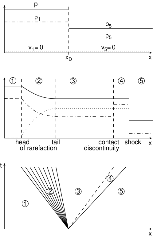
Figure 1: Schematic solution of a Riemann problem in special relativistic hydrodynamics. The initial state at $t=0$ (top figure) consists of two constant states (1) and (5) with $p_{1}>p_{5}$, $\rho_{1}>\rho_{5}$ and $v_{1}=v_{2}=0$ separated by a diaphragm at $x_{\rm D}$. The evolution of the flow pattern once the diaphragm is removed (middle figure) is illustrated in a space–time diagram (bottom figure) with a shock wave (solid line) and a contact discontinuity (dashed line) moving to the right. The bundle of solid lines represents a rarefaction wave propagating to the left.

The fact that one Riemann invariant is constant through any rarefaction wave provides the relation needed to derive the function ${\cal R}^{S}$

$${\cal R}^{S}(p)=\frac{(1+v_{S})A_{\pm}(p)-(1-v_{S})}{(1+v_{S})A_{\pm}(p)+(1-v_{S})}$$ (16)

with

$$A_{\pm}(p)=\left(\frac{\sqrt{\gamma-1}-c(p)}{\sqrt{\gamma-1}+c(p)}\frac{\sqrt{\gamma-1}+c_{S}}{\sqrt{\gamma-1}-c_{S}}\right)^{\pm\frac{2}{\sqrt{\gamma-1}}}$$ (17)

the $+$ ($-$) sign of $A_{\pm}$ corresponding to $S=L$ ($S=R$). In the above equation, $c_{S}$ is the sound speed of the state ${\bf v}_{S}$, and $c(p)$ is given by

$$c(p)=\left(\frac{\gamma(\gamma-1)p}{(\gamma-1)\rho_{S}(p/p_{S})^{1/\gamma}+\gamma p}\right)^{1/2}\,.$$ (18)

The family of all states ${\cal S}^{S}(p)$, which can be connected through a shock with a given state ${\bf v}_{S}$ ahead of the wave, is determined by the shock jump conditions. One obtains

$${\cal S}^{S}(p) = \left(h_{S}W_{S}v_{S}\pm\frac{p-p_{S}}{j(p)\sqrt{1-V_{\pm}(p)^{2}}}\right)$$ (19)

$$\left[h_{S}W_{S}+(p-p_{S})\left(\frac{1}{\rho_{S}W_{S}}\pm\frac{v_{S}}{j(p)\sqrt{1-V_{\pm}(p)^{2}}}\right)\right]^{-1}\,,$$

where the $+$ ($-$) sign corresponds to $S=R$ ($S=L$). $V_{\pm}(p)$ and $j(p)$ denote the shock velocity and the modulus of the mass flux across the shock front, respectively. They are given by

$$V_{\pm}(p)=\frac{\rho_{S}^{2}W_{S}^{2}v_{S}\pm j(p)^{2}\sqrt{1+(\rho_{S}/j(p))^{2}}}{\rho_{S}^{2}W_{S}^{2}+j(p)^{2}}\,,$$ (20)

and

$$j(p)=\sqrt{\frac{p_{S}-p}{{\displaystyle\frac{h_{S}^{2}-h(p)^{2}}{p_{S}-p}-\frac{2h_{S}}{\rho_{S}}}}}\,,$$ (21)

where the enthalpy $h(p)$ of the state behind the shock is the (unique) positive root of the quadratic equation

$$\left(1+\frac{(\gamma-1)(p_{S}-p)}{\gamma p}\right)h^{2}-\frac{(\gamma-1)(p_{S}-p)}{\gamma p}h+\frac{h_{S}(p_{S}-p)}{\rho_{S}}-h_{S}^{2}=0\,,$$ (22)

which is obtained from the Taub adiabat (the relativistic version of the Hugoniot adiabat) for an ideal gas equation of state.

Figure 2: Graphical solution in the $p$–$v$ plane of the Riemann problems defined by the initial states $(p_{\rm L}=10^{3},\,\rho_{\rm L}=1,\,v_{\rm L}=0.5)$ and $(p_{\rm R}^{i},\,\rho_{\rm R}=1,\,v_{\rm R}=0)$ with $i=1,2,3,4$, where $p_{\rm R}^{1}=10^{2}$, $p_{\rm R}^{2}=10$, $p_{\rm R}^{3}=1$, and $p_{\rm R}^{4}=10^{-1}$, respectively. The adiabatic index of the fluid is $5/3$ in all cases. Note the asymptotic behavior of the functions as they approach $v=1$ (i.e., the speed of light).

The functions $v_{\rm L*}(p)$ and $v_{\rm R*}(p)$ are displayed in Fig. 2 in a $p$–$v$ diagram for a particular set of Riemann problems. Once $p_{*}$ has been obtained, the remaining state quantities and the complete Riemann solution,

$${\bf u}={\bf u}(\frac{x-x_{0}}{t-t_{0}};{\bf u}_{\rm L},{\bf u}_{\rm R})),$$ (23)

can easily be derived.

In Section 9.3 we provide a FORTRAN program called RIEMANN, which allows one to compute the exact solution of an arbitrary special relativistic Riemann problem using the algorithm just described.

The treatment of multidimensional special relativistic flows is significantly more difficult than that of multidimensional Newtonian flows. In SRHD all components (normal and tangential) of the flow velocity are strongly coupled through the Lorentz factor, which complicates the solution of the Riemann problem severely. For shock waves, this coupling ’only’ increases the number of algebraic jump conditions, which must be solved. However, for rarefactions it implies the solution of a system of ordinary differential equations [105].

3 HIGH-RESOLUTION SHOCK-CAPTURING
METHODS

The application of high-resolution shock-capturing (HRSC) methods caused a revolution in numerical SRHD. These methods satisfy in a quite natural way the basic properties required for any acceptable numerical method: (i) high order of accuracy, (ii) stable and sharp description of discontinuities, and (iii) convergence to the physically correct solution. Moreover, HRSC methods are conservative, and because of their shock capturing property discontinuous solutions are treated both consistently and automatically whenever and wherever they appear in the flow.

As HRSC methods are written in conservation form, the time evolution of zone averaged state vectors is governed by some functions (the numerical fluxes) evaluated at zone interfaces. Numerical fluxes are mostly obtained by means of an exact or approximate Riemann solver. High resolution is usually achieved by using monotonic polynomials in order to interpolate the approximate solutions within numerical cells.

Solving Riemann problems exactly involves time–consuming computations, which are particularly costly in the case of multidimensional SRHD due to the coupling of the equations through the Lorentz factor (see Section 2.3). Therefore, as an alternative, the usage of approximate Riemann solvers has been proposed.

In this Section we summarize the computation of the numerical fluxes in a number of methods for numerical SRHD. Methods based on exact Riemann solvers are discussed in Sections 3.1 and 3.2, while those based on approximate solvers are discussed in Sections (3.3 – 3.7) Readers not familiar with HRSC methods are referred to Section 9.4, where the basic properties of these methods as well as an outline of the recent developments are described.

3.1 Relativistic PPM

Martí & Müller [106] have used the procedure discussed in Section 2.3 to construct an exact Riemann solver, which they then incorporated in an extension of the PPM method [32] for 1D SRHD. In their relativistic PPM method numerical fluxes are calculated according to

$${\widehat{\bf F}}^{\rm RPPM}={\bf F}({\bf u}(0;{\bf u}_{\rm L},{\bf u}_{\rm R}))\,,$$ (24)

where ${\bf u}_{L}$ and ${\bf u}_{R}$ are approximations of the state vector at the left and right side of a zone interface obtained by a second–order accurate interpolation in space and time, and ${\bf u}(0;{\bf u}_{\rm L},{\bf u}_{\rm R})$ is the solution of the Riemann problem defined by the two interpolated states at the position of the initial discontinuity.

The PPM interpolation algorithm described in [32] gives monotonic conservative parabolic profiles of variables within a numerical zone. In the relativistic version of PPM the original interpolation algorithm is applied to zone averaged values of the primitive variables ${\bf v}=(p,\rho,v)$, which are obtained from zone averaged values of the conserved quantities ${\bf u}$. For each zone $j$, the quartic polynomial with zone–averaged values $a_{j-2}$, $a_{j-1}$, $a_{j}$, $a_{j+1}$, and $a_{j+2}$ (where $a=\rho,p,v$) is used to interpolate the structure inside the zone. In particular, the values of $a$ at the left and right interface of the zone, $a_{L,j}$ and $a_{R,j}$, are obtained this way. These reconstructed values are then modified such that the parabolic profile, which is uniquely determined by $a_{L,j}$, $a_{R,j}$ and $a_{j}$, is monotonic inside the zone.

The time–averaged fluxes at an interface $j+1/2$ separating zones $j$ and $j+1$ are computed from two spatially averaged states, ${\bf v}_{j+\frac{1}{2},L}$ and ${\bf v}_{j+\frac{1}{2},R}$ at the left and right side of the interface, respectively. These left and right states are constructed taking into account the characteristic information reaching the interface from both sides during the time step. In the relativistic version of PPM the same procedure as in [32] has been followed using the characteristic speeds and Riemann invariants of the equations of relativistic hydrodynamics.

3.2 Relativistic Glimm’s method

Wen et al. [182] have extended Glimm’s random choice method [65] to 1D SRHD. They developed a first–order accurate hydrodynamic code combining Glimm’s method (using an exact Riemann solver) with standard finite difference schemes.

In the random choice method, given two adjacent states, ${\bf u}_{j}^{n}$ and ${\bf u}_{j+1}^{n}$, at time $t^{n}$, the value of the numerical solution at time $t^{n+1/2}$ and position $x_{j+1/2}$ is given by the exact solution ${\bf u}(x,t)$ of the Riemann problem evaluated at a randomly chosen point inside zone $(j,j+1)$, i.e.,

$${\bf u}_{j+\frac{1}{2}}^{n+\frac{1}{2}}={\bf u}\left(\frac{(j+\xi_{n})\Delta x}{(n+\frac{1}{2})\Delta t};\,{\bf u}_{j}^{n},\,{\bf u}_{j+1}^{n}\right)\,,$$ (25)

where $\xi_{n}$ is a random number in the interval $[0,1]$.

Besides being conservative on average, the main advantages of Glimm’s method are that it produces both completely sharp shocks and contact discontinuities, and that it is free of diffusion and dispersion errors.

Chorin [28] applied Glimm’s method to the numerical solution of homogeneous hyperbolic conservation laws. Colella [30] proposed an accurate procedure of randomly sampling the solution of local Riemann problems and investigated the extension of Glimm’s method to two dimensions using operator splitting methods.

3.3 Two-shock approximation for relativistic hydrodynamics

This approximate Riemann solver is obtained from a relativistic extension of Colella’s method [30] for classical fluid dynamics, where it has been shown to handle shocks of arbitrary strength [30, 186]. In order to construct Riemann solutions in the two–shock approximation one analytically continues shock waves towards the rarefaction side (if present) of the zone interface instead of using an actual rarefaction wave solution. Thereby one gets rid of the coupling of the normal and tangential components of the flow velocity (see Section 2.3), and the remaining minor algebraic complications are the Rankine–Hugoniot conditions across oblique shocks. Balsara [8] has developed an approximate relativistic Riemann solver of this kind by solving the jump conditions in the shocks’ rest frames in the absence of transverse velocities, after appropriate Lorentz transformations. Dai & Woodward [35] have developed a similar Riemann solver based on the jump conditions across oblique shocks making the solver more efficient.

Table 1 gives the converged solution for the intermediate states obtained with both Balsara’s and Dai’s & Woodward’s procedure for the case of the Riemann problems defined in Section 6.2 (involving strong rarefaction waves) together with the exact solution. Despite the fact that both approximate methods involve very different algebraic expressions, their results differ by less than $2\%$. However, the discrepancies are much larger when compared with the exact solution (up to a $100\%$ error in the density of the left intermediate state in Problem 2). The accuracy of the two–shock approximation should be tested in the ultra-relativistic limit, where the approximation can produce large errors in the Lorentz factor (in the case of Riemann problems involving strong rarefaction waves) with important implications for the fluid dynamics. Finally, the suitability of the two–shock approximation for Riemann problems involving transversal velocities still needs to be tested.

Table 1: Pressure $p_{*}$, velocity $v_{*}$ and densities $\rho_{\rm L*}$ (left), $\rho_{\rm R*}$ (right) for the intermediate state obtained for the two–shock approximation of Balsara [8] (B) and of Dai & Woodward [35] (DW) compared to the exact solution (Exact) for the Riemann problems defined in Sect. 6.2.

Method	$p_{*}$	$v_{*}$	$\rho_{\rm L*}$	$\rho_{\rm R*}$
Problem 1
B	1.440E+00	7.131E–01	2.990E+00	5.069E+00
DW	1.440E+00	7.131E–01	2.990E+00	5.066E+00
Exact	1.445E+00	7.137E–01	2.640E+00	5.062E+00
Problem 2
B	1.543E+01	9.600E–01	7.325E–02	1.709E+01
DW	1.513E+01	9.608E–01	7.254E–02	1.742E+01
Exact	1.293E+01	9.546E–01	3.835E–02	1.644E+01

3.4 Roe-type relativistic solvers

Linearized Riemann solvers are based on the exact solution of Riemann problems of a modified system of conservation equations obtained by a suitable linearization of the original system. This idea was put forward by Roe [151], who developed a linearized Riemann solver for the equations of ideal (classical) gas dynamics. Eulderink et al. [50, 51] have extended Roe’s Riemann solver to the general relativistic system of equations in arbitrary spacetimes. Eulderink uses a local linearization of the Jacobian matrices of the system fulfilling the properties demanded by Roe in his original paper.

Let ${\cal B}=\partial{\bf F}/\partial{\bf u}$ be the Jacobian matrix associated with one of the fluxes ${\bf F}$ of the original system, and ${\bf u}$ the vector of unknowns. Then, the locally constant matrix $\widetilde{\cal B}$, depending on ${\bf u}_{\rm L}$ and ${\bf u}_{\rm R}$ (the left and right state defining the local Riemann problem) must have the following four properties:

• 1. It constitutes a linear mapping from the vector space ${\bf u}$ to the vector space ${\bf F}$.

• 2. As ${\bf u}_{\rm L}\rightarrow{\bf u}_{\rm R}\rightarrow{\bf u},\;\widetilde{\cal B}({\bf u}_{\rm L},{\bf u}_{\rm R})\rightarrow{\cal B}({\bf u})$.

• 3. For any ${\bf u}_{\rm L}$, ${\bf u}_{\rm R},\;\widetilde{\cal B}({\bf u}_{\rm L},{\bf u}_{\rm R})({\bf u}_{\rm R}-{\bf u}_{\rm L})={\bf F}({\bf u}_{\rm R})-{\bf F}({\bf u}_{\rm L})$.

• 4. The eigenvectors of $\widetilde{\cal B}$ are linearly independent.

Conditions 1 and 2 are necessary if one is to recover smoothly the linearized algorithm from the nonlinear version. Condition 3 (supposing 4 is fulfilled) ensures that if a single discontinuity is located at the interface, then the solution of the linearized problem is the exact solution of the nonlinear Riemann problem.

Once a matrix, $\widetilde{\cal B}$, satisfying Roe’s conditions has been obtained for every numerical interface, the numerical fluxes are computed by solving the locally linear system. Roe’s numerical flux is then given by

$${\widehat{\bf F}}^{\rm ROE}=\frac{1}{2}\left[{\bf F}({\bf u}_{\rm L})+{\bf F}({\bf u}_{\rm R})-\sum_{p}|\widetilde{\lambda}^{(p)}|\widetilde{\alpha}^{(p)}\widetilde{\bf r}^{(p)}\right]\,,$$ (26)

with

$$\widetilde{\alpha}^{(p)}=\widetilde{\bf l}^{(p)}\cdot({\bf u}_{\rm R}-{\bf u}_{\rm L})\,,$$ (27)

where $\widetilde{\lambda}^{(p)}$, $\widetilde{\bf r}^{(p)}$, and $\widetilde{\bf l}^{(p)}$ are the eigenvalues and the right and left eigenvectors of $\widetilde{\cal B}$, respectively ($p$ runs from 1 to the number of equations of the system).

Roe’s linearization for the relativistic system of equations in a general spacetime can be expressed in terms of the average state [50, 51]

$$\widetilde{\bf w}=\frac{{\bf w}_{\rm L}+{\bf w}_{\rm R}}{k_{\rm L}+k_{\rm R}}$$ (28)

with

$${\bf w}=(ku^{0},ku^{1},ku^{2},ku^{3},k\frac{p}{\rho h})$$ (29)

and

$$k^{2}=\sqrt{-g}\rho h\,,$$ (30)

where $g$ is the determinant of the metric tensor $g_{\mu\nu}$. The role played by the density ${\rho}$ in case of the Cartesian non-relativistic Roe solver as a weight for averaging, is taken over in the relativistic variant by $k$, which apart from geometrical factors tends to $\rho$ in the non-relativistic limit. A Riemann solver for special relativistic flows and the generalization of Roe’s solver to the Euler equations in arbitrary coordinate systems are easily deduced from Eulderink’s work. The results obtained in 1D test problems for ultra-relativistic flows (up to Lorentz factors 625) in the presence of strong discontinuities and large gravitational background fields demonstrate the excellent performance of the Eulderink-Roe solver [51].

Relaxing condition 3 above, Roe’s solver is no longer exact for shocks but still produces accurate solutions, and moreover, the remaining conditions are fulfilled by a large number of averages. The 1D general relativistic hydrodynamic code developed by Romero et al. [153] uses flux formula (26) with an arithmetic average of the primitive variables at both sides of the interface. It has successfully passed a long series of tests including the spherical version of the relativistic shock reflection (see Section 6.1).

Roe’s original idea has been exploited in the so–called local characteristic approach (see, e.g., [193]). This approach relies on a local linearization of the system of equations by defining at each point a set of characteristic variables, which obey a system of uncoupled scalar equations. This approach has proven to be very successful, because it allows for the extension to systems of scalar nonlinear methods. Based on the local characteristic approach are the methods developed by Marquina et al. [103] and Dolezal & Wong [41], which both use high–order reconstructions of the numerical characteristic fluxes, namely PHM [103] and ENO [41] (see Section 9.4).

3.5 Falle and Komissarov upwind scheme

Instead of starting from the conservative form of the hydrodynamic equations, one can use a primitive–variable formulation in quasi-linear form

$$\frac{\partial{\bf v}}{\partial t}+{\cal A}\frac{\partial{\bf v}}{\partial x}=0\,,$$ (31)

where ${\bf v}$ is any set of primitive variables. A local linearization of the above system allows one to obtain the solution of the Riemann problem, and from this the numerical fluxes needed to advance a conserved version of the equations in time.

Falle & Komissarov [55] have considered two different algorithms to solve the local Riemann problems in SRHD by extending the methods devised in [53]. In a first algorithm, the intermediate states of the Riemann problem at both sides of the contact discontinuity, ${\bf v}_{L*}$ and ${\bf v}_{R*}$, are obtained by solving the system

$${\bf v}_{\rm L*}={\bf v}_{\rm L}+b_{\rm L}{\bf r}^{-}_{\rm L}\,,\;\;{\bf v}_{\rm R*}={\bf v}_{\rm R}+b_{\rm R}{\bf r}^{+}_{\rm R}\,,$$ (32)

where ${\bf r}^{-}_{\rm L}$ is the right eigenvector of ${\cal A}({\bf v}_{\rm L})$ associated with sound waves moving upstream and ${\bf r}^{+}_{\rm R}$ is the right eigenvector of ${\cal A}({\bf v}_{\rm R})$ of sound waves moving downstream. The continuity of pressure and of the normal component of the velocity across the contact discontinuity allows one to obtain the wave strengths $b_{L}$ and $b_{R}$ from the above expressions, and hence the linear approximation to the intermediate state ${\bf v}_{*}({\bf v}_{\rm L},{\bf v}_{\rm R})$.

In the second algorithm proposed by Falle & Komissarov [55], a linearization of system (31) is obtained by constructing a constant matrix $\widetilde{\cal A}({\bf v}_{\rm L},{\bf v}_{\rm R})={\cal A}(\frac{1}{2}({\bf v}_{\rm L}+{\bf v}_{\rm R}))$. The solution of the corresponding Riemann problem is that of a linear system with matrix $\widetilde{\cal A}$, i.e.,

$${\bf v}_{*}={\bf v}_{\rm L}+\sum_{\widetilde{\lambda}^{(p)}<0}\widetilde{\alpha}^{(p)}\,\widetilde{\bf r}^{(p)}\,,$$ (33)

or, equivalently,

$${\bf v}_{*}={\bf v}_{\rm R}-\sum_{\widetilde{\lambda}^{(p)}>0}\widetilde{\alpha}^{(p)}\,\widetilde{\bf r}^{(p)})\,,$$ (34)

with

$$\widetilde{\alpha}^{(p)}=\widetilde{\bf l}^{(p)}\cdot({\bf v}_{\rm R}-{\bf v}_{\rm L})\,,$$ (35)

where $\widetilde{\lambda}^{(p)}$, $\widetilde{\bf r}^{(p)}$, and $\widetilde{\bf l}^{(p)}$ are the eigenvalues and the right and left eigenvectors of $\widetilde{\cal A}$, respectively ($p$ runs from 1 to the number of equations of the system).

In both algorithms, the final step involves the computation of the numerical fluxes for the conservation equations

$${\widehat{\bf F}}^{\rm FK}={\bf F}({\bf u}({\bf v}_{*}({\bf v}_{\rm L},{\bf v}_{\rm R})))\,.$$ (36)

3.6 Relativistic HLL Method

Schneider et al. [157] have proposed to use the method of Harten, Lax & van Leer (HLL hereafter [74]) to integrate the equations of SRHD. This method avoids the explicit calculation of the eigenvalues and eigenvectors of the Jacobian matrices and is based on an approximate solution of the original Riemann problems with a single intermediate state

$${\bf u}^{\rm HLL}(x/t;{\bf u}_{\rm L},{\bf u}_{\rm R})=\left\{\begin{array}[]{ll}{\bf u}_{\rm L}&\mbox{for $x<a_{\rm L}t$}\\ {\bf u}_{*}&\mbox{for $a_{\rm L}t\leq x\leq a_{\rm R}t$}\\ {\bf u}_{\rm R}&\mbox{for $x>a_{\rm R}t$}\end{array}\right.\,,$$ (37)

where $a_{\rm L}$ and $a_{\rm R}$ are lower and upper bounds for the smallest and largest signal velocities, respectively. The intermediate state ${\bf u}_{*}$ is determined by requiring consistency of the approximate Riemann solution with the integral form of the conservation laws in a grid zone. The resulting integral average of the Riemann solution between the slowest and fastest signals at some time is given by

$${\bf u}_{*}=\frac{a_{\rm R}{\bf u}_{\rm R}-a_{\rm L}{\bf u}_{\rm L}-{\bf F}({\bf u}_{\rm R})+{\bf F}({\bf u}_{\rm L})}{a_{\rm R}-a_{\rm L}}\,,$$ (38)

and the numerical flux by

$${\widehat{\bf F}}^{\rm HLL}=\frac{a_{\rm R}^{+}{\bf F}({\bf u}_{\rm L})-a_{\rm L}^{-}{\bf F}({\bf u}_{\rm R})+a_{\rm R}^{+}a_{\rm L}^{-}({\bf u}_{\rm R}-{\bf u}_{\rm L})}{a_{\rm R}^{+}-a_{\rm L}^{-}}\,,$$ (39)

where

$$a_{\rm L}^{-}={\rm min}\{0,a_{\rm L}\}\,,\;\;a_{\rm R}^{+}={\rm max}\{0,a_{\rm R}\}\,.$$ (40)

An essential ingredient of the HLL scheme are good estimates for the smallest and largest signal velocities. In the non-relativistic case, Einfeldt [49] proposed calculating them based on the smallest and largest eigenvalues of Roe’s matrix. This HLL scheme with Einfeldt’s recipe is a very robust upwind scheme for the Euler equations and possesses the property of being positively conservative. The method is exact for single shocks, but it is very dissipative, especially at contact discontinuities.

Schneider et al. [157] have presented results in 1D ultra-relativistic hydrodynamics using a version of the HLL method with signal velocities given by

$$a_{\rm R}=(\bar{v}+\bar{c}_{s})/(1+\bar{v}\bar{c}_{s})\,,$$ (41)

$$a_{\rm L}=(\bar{v}-\bar{c}_{s})/(1-\bar{v}\bar{c}_{s})\,,$$ (42)

where $c_{s}$ is the relativistic sound speed, and where the bar denotes the arithmetic mean between the initial left and right states. Duncan & Hughes [46] have generalized this method to 2D SRHD and applied it to the simulation of relativistic extragalactic jets.

3.7 Marquina’s flux formula

Godunov–type schemes are indeed very robust in most situations although they fail spectacularly on occasions. Reports on approximate Riemann solver failures and their respective corrections (usually a judicious addition of artificial dissipation) are abundant in the literature [149]. Motivated by the search for a robust and accurate approximate Riemann solver that avoids these common failures, Donat & Marquina [43] have extended to systems a numerical flux formula which was first proposed by Shu & Osher [159] for scalar equations. In the scalar case and for characteristic wave speeds which do not change sign at the given numerical interface, Marquina’s flux formula is identical to Roe’s flux. Otherwise, the scheme switches to the more viscous, entropy satisfying local Lax–Friedrichs scheme [159]. In the case of systems, the combination of Roe and local–Lax–Friedrichs solvers is carried out in each characteristic field after the local linearization and decoupling of the system of equations [43]. However, contrary to Roe’s and other linearized methods, the extension of Marquina’s method to systems is not based on any averaged intermediate state.

Martí et al. have used this method in their simulations of relativistic jets [107, 108]. The resulting numerical code has been successfully used to describe ultra-relativistic flows in both one and two spatial dimensions with great accuracy (a large set of test calculations using Marquina’s Riemann solver can be found in Appendix II of [108]). Numerical experimentation in two dimensions confirms that the dissipation of the scheme is sufficient to eliminate the carbuncle phenomenon [149], which appears in high Mach number relativistic jet simulations when using other standard solvers [42]. Aloy et al. [2] have implemented Marquina’s flux formula in their three dimensional relativistic hydrodynamic code GENESIS. Font et al. [59] have developed a 3D general relativistic hydro code where the matter equations are integrated in conservation form and fluxes are calculated with Marquina’s formula.

3.8 Symmetric TVD schemes with nonlinear numerical dissipation

The methods discussed in the previous subsections are all based on exact or approximate solutions of Riemann problems at cell interfaces in order to stabilize the discretization scheme across strong shocks. Another successful approach relies on the addition of nonlinear dissipation terms to standard finite difference methods. The algorithm of Davis [37] is based on such an approach. It can be interpreted as a Lax–Wendroff scheme with a conservative TVD dissipation term. The numerical dissipation term is local, free of problem dependent parameters and does not require any characteristic information. This last fact makes the algorithm extremely simple when applied to any hyperbolic system of conservation laws.

A relativistic version of Davis’ method has been used by Koide et al. [81, 80, 126] in 2D and 3D simulations of relativistic magneto–hydrodynamic jets with moderate Lorentz factors. Although the results obtained are encouraging, the coarse grid zoning used in these simulations and the relative smallness of the beam flow Lorentz factor (4.56, beam speed $\approx 0.98c$) does not allow for a comparison with Riemann–solver–based HRSC methods in the ultra-relativistic limit.

4 OTHER DEVELOPMENTS

4.1 Van Putten’s approach

Relying on a formulation of Maxwell’s equations as a hyperbolic system in divergence form, van Putten [173] has devised a numerical method to solve the equations of relativistic ideal MHD in flat spacetime [175]. Here we only discuss the basic principles of the method in one spatial dimension. In van Putten’s approach, the state vector ${\bf u}$ and the fluxes ${\bf F}$ of the conservation laws are decomposed into a spatially constant mean (subscript 0) and a spatially dependent variational (subscript 1) part

$${\bf u}(t,x)={\bf u}_{0}(t)+{\bf u}_{1}(t,x)\,,\;\;{\bf F}(t,x)={\bf F}_{0}(t)+{\bf F}_{1}(t,x)\,.$$ (43)

The RMHD equations then become a system of evolution equations for the integrated variational parts ${\bf u_{1}}^{*}$, which reads

$$\frac{\partial{\bf u_{1}}^{*}}{\partial t}+{\bf F_{1}}=0\,,$$ (44)

together with the conservation condition

$$\frac{d{\bf F}_{0}}{dt}=0\,.$$ (45)

The quantities ${\bf u_{1}}^{*}$ are defined as

$${\bf u_{1}}^{*}(t,x)=\int^{x}{\bf u_{1}}(t,y)\,\,dy\,.$$ (46)

They are continuous and standard methods can be used to integrate the system (44). Van Putten uses a leapfrog method.

The new state vector ${\bf u}(t,x)$ is then obtained from ${\bf u_{1}}^{*}(t,x)$ by numerical differentiation. This process can lead to oscillations in the case of strong shocks and a smoothing algorithm should be applied. Details of this smoothing algorithm and of the numerical method in one and two spatial dimensions can be found in [174] together with results on a large variety of tests.

Van Putten has applied his method to simulate relativistic hydrodynamic and magneto hydrodynamic jets with moderately flow Lorentz factors ($<4.25$) [176, 179].

4.2 Relativistic SPH

Besides finite volume schemes, another completely different method is widely used in astrophysics for integrating the hydrodynamic equations. This method is Smoothed Particle Hydrodynamics, or SPH for short ([97, 63, 119]). The fundamental idea of SPH is to represent a fluid by a Monte Carlo sampling of its mass elements. The motion and thermodynamics of these mass elements is then followed as they move under the influence of the hydrodynamics equations. Because of its Lagrangian nature there is no need within SPH for explicit integration of the continuity equation, but in some implementations of SPH this is done nevertheless for certain reasons. As both the equation of motion of the fluid and the energy equation involve continuous properties of the fluid and their derivatives, it is necessary to estimate these quantities from the positions, velocities and internal energies of the fluid elements, which can be thought of as particles moving with the flow. This is done by treating the particle positions as a finite set of interpolating points where the continuous fluid variables and their gradients are estimated by an appropriately weighted average over neighbouring particles. Hence, SPH is a free-Lagrange method, i.e., spatial gradients are evaluated without the use of a computational grid.

A comprehensive discussion of SPH can be found in the reviews of Hernquist & Katz [76], Benz [11] and Monaghan [118, 119]. The non-relativistic SPH equations are briefly discussed in Section (9.5). The capabilities and limits of SPH are explored, e.g., in [164, 167], and the stability of the SPH algorithm is investigated in [165].

The SPH equations for special relativistic flows have been first formulated by Monaghan [118]. For such flows the SPH equations given in Section (9.5) can be taken over except that each SPH particle $a$ carries $\nu_{a}$ baryons instead of mass $m_{a}$ [118, 29]. Hence, the rest mass of particle $a$ is given by $m_{a}=m_{0}\nu_{a}$, where $m_{0}$ is the baryon rest mass (if the fluid is made of baryons). Transforming the notation used in [29] to ours, the continuity equation, the momentum and the total energy equations for particle $a$ are given by (unit of velocity is $c$)

$${dN_{a}\over dt}=-\sum_{b}\nu_{b}({\mathbf{v}}_{a}-{\mathbf{v}}_{b})\cdot\nabla_{a}W_{ab}\;,$$ (47)

$${d\widehat{\mathbf{S}}_{a}\over dt}=-\sum_{b}\nu_{b}\left({p_{a}\over N_{a}^{2}}+{p_{b}\over N_{b}^{2}}+{\mathbf{\Pi}}_{ab}\right)\cdot\nabla_{a}W_{ab}\;,$$ (48)

and

$${d\widehat{\tau}_{a}\over dt}=-\sum_{b}\nu_{b}\left({p_{a}{\mathbf{v}}_{a}\over N_{a}^{2}}+{p_{b}{\mathbf{v}}_{b}\over N_{b}^{2}}+{\mathbf{\Omega}}_{ab}\right)\cdot\nabla_{a}W_{ab}\;,$$ (49)

respectively. Here, the summation is over all particles other than particle $a$, and $d/dt$ denotes the Lagrangian time derivative. $N=D/m_{0}$ is the baryon number density,

$$\widehat{\mathbf{S}}\equiv\frac{{\mathbf{S}}}{N}=m_{0}hW{\mathbf{v}}$$ (50)

the momentum per particle, and

$$\widehat{\tau}\equiv\frac{\tau}{N}+m_{0}=m_{0}hW-\frac{p}{N}$$ (51)

the total energy per particle (all measured in the laboratory frame). The momentum density ${\mathbf{S}}\equiv(S^{1},S^{2},S^{3})^{T}$, the energy density $\tau$ (measured in units of the rest mass energy density), and the specific enthalpy $h$ are defined in Section (2.1). ${\mathbf{\Pi}}_{ab}$ and ${\mathbf{\Omega}}_{ab}$ are the SPH dissipation terms, and $\nabla_{a}W_{ab}$ denotes the gradient of the kernel $W_{ab}$ (see Section (9.5) for more details).

Special relativistic flow problems have been simulated with SPH by [89, 79, 99, 100, 29, 160]. Extensions of SPH capable of treating general relativistic flows have been considered by [79, 88, 160]. Concerning relativistic SPH codes the artificial viscosity is the most critical issue. It is required to handle shock waves properly, and ideally it should be predicted by a relativistic kinetic theory for the fluid. However, unlike its Newtonian analogue, the relativistic theory has not yet been developed to the degree required to achieve this. For Newtonian SPH Lattanzio et al. [93] have shown that a viscosity quadratic in the velocity divergence is necessary in high Mach number flows. They proposed a form such that the viscous pressure could be simply added to the fluid pressure in the equation of motion and the energy equation. Because this simple form of the artificial viscosity has known limitations, they also proposed a more sophisticated form of the artificial viscosity terms, which leads to a modified equation of motion. This artificial viscosity works much better, but it cannot be generalized to the relativistic case in a consistent way. Utilizing an equation for the specific internal energy both Mann [99] and Laguna et al. [88] use such an inconsistent formulation. Their artificial visocity term is not included into the expression of the specific relativistic enthalpy. In a second approach, Mann [99] allows for a time–dependent smoothing length and SPH particle mass, and further proposed a SPH variant based on the total energy equation. Lahy [89] and Siegler & Riffert [160] use a consistent artificial viscosity pressure added to the fluid pressure. Siegler & Riffert [160] have also formulated the hydrodynamic equations in conservation form.

Monaghan [120] incorporates concepts from Riemann solvers into SPH. For this reason he also proposes to use a total energy equation in SPH simulation instead of the commonly used internal energy equation, which would involve time derivatives of the Lorentz factor in the relativistic case. Chow & Monaghan [29] have extended this concept and have proposed an SPH algorithm, which gives good results when simulating an ultra-relativistic gas. In both cases the intention was not to introduce Riemann solvers into the SPH algorithm, but to use them as a guide to improve the artificial viscosity required in SPH.

In Roe’s Riemann solver [151], as well as in its relativistic variant proposed by Eulerdink [50, 51] (see Section 3.4), the numerical flux is computed by solving a locally linear system and depends on both the eigenvalues and (left and right) eigenvectors of the Jacobian matrix associated to the fluxes and on the jumps in the conserved physical variables (see Eqs. 26 and 27). Monaghan [120] realized that an appropriate form of the dissipative terms ${\mathbf{\Pi}}_{ab}$ and ${\mathbf{\Omega}}_{ab}$ for the interaction between particles $a$ and $b$ can be obtained by treating the particles as the equivalent of left and right states taken with reference to the line joining the particles. The quantity corresponding to the eigenvalues (wave propagation speeds) is an appropriate signal velocity $v_{sig}$ (see below), and that equivalent to the jump across characteristics is a jump in the relevant physical variable. For the artificial viscosity tensor, ${\mathbf{\Pi}}_{ab}$, Monaghan [120] assumes that the jump in velocity across characteristics can be replaced by the velocity difference between $a$ and $b$ along the line joining them.

With these considerations in mind Chow & Monaghan [29] proposed for ${\mathbf{\Pi}}_{ab}$ in the relativistic case the form

$${\mathbf{\Pi}}_{ab}=-\frac{Kv_{sig}(\widehat{\mathbf{S}}_{a}^{\ast}-\widehat{\mathbf{S}}_{b}^{\ast})\cdot{\mathbf{j}}}{\overline{N}_{ab}}\;,$$ (52)

when particles $a$ and $b$ are approaching, and ${\mathbf{\Pi}}_{ab}=0$ otherwise. Here $K=0.5$ is a dimensionless parameter, which is chosen to have the same value as in the non-relativistic case [120]. $\overline{N}_{ab}=(N_{a}+N_{b})/2$ is the average baryon number density, which has to be present in (52), because the pressure terms in the summation of (85) have an extra density in the denominator arising from the SPH interpolation. Furthermore,

$${\mathbf{j}}=\frac{{\mathbf{r}}_{ab}}{|{\mathbf{r}}_{ab}|}$$ (53)

is the unit vector from $b$ to $a$, and

$$\widehat{\mathbf{S}}^{\ast}=m_{0}hW^{\ast}{\mathbf{v}}\;,$$ (54)

where

$$W^{\ast}=\frac{1}{\sqrt{1-({\mathbf{v}}\cdot{\mathbf{j}})^{2}}}\;.$$ (55)

Using instead of $\widehat{\mathbf{S}}$ (see Eq. 50) the modified momentum $\widehat{\mathbf{S}}^{\ast}$, which involves the line of sight velocity ${\mathbf{v}}\cdot{\mathbf{j}}$, guarantees that the viscous dissipation is positive definite [29].

The dissipation term in the energy equation is derived in a similar way and is given by [29]

$${\mathbf{\Omega}}_{ab}=-\frac{Kv_{sig}(\widehat{\tau}_{a}^{\ast}-\widehat{\tau}_{b}^{\ast})\,{\mathbf{j}}}{\overline{N}_{ab}}\;,$$ (56)

if $a$ and $b$ are approaching, and ${\mathbf{\Omega}}_{ab}=0$ otherwise. ${\mathbf{\Omega}}_{ab}$ involves the energy $\widehat{\tau}^{\ast}$, which is identical to $\widehat{\tau}$ (see Eq. 51) except that $W$ is replaced by $W^{\ast}$.

To determine the signal velocity Chow & Monaghan [29] (and Monaghan [120] in the non-relativistic case) start from the (local) eigenvalues, and hence the wave velocities $(v\pm c_{s})/(1\pm vc_{s})$ and $v$ of one–dimensional relativistic hydrodynamic flows. Again considering particles $a$ and $b$ as the left and right states of a Riemann problem with respect to motions along the line joining the particles, the appropriate signal velocity is the speed of approach (as seen in the computing frame) of the signal sent from $a$ towards $b$ and that from $b$ to $a$. This is the natural speed for the sharing of physical quantities, because when information about the two states meets it is time to construct a new state. This speed of approach should be used when determining the size of the time step by the Courant condition (for further details see [29]).

Chow & Monaghan [29] have demonstrated the performance of their Riemann problem guided relativistic SPH algorithm by calculating several shock tube problems involving ultra-relativistic speeds up to $v=0.9999$. The algorithm gives good results, but finite volume schemes based on Riemann solvers give more accurate results and can handle even larger speeds (see Section 6).

4.3 Relativistic beam scheme

Sanders & Prendergast [155] proposed an explicit scheme to solve the equilibrium limit of the non-relativistic Boltzmann equation, i.e., the Euler equations of Newtonian fluid dynamics. In their so–called beam scheme the Maxwellian velocity distribution function is approximated by several Dirac delta functions or discrete beams of particles in each computational cell, which reproduce the appropriate moments of the distribution function. The beams transport mass, momentum and energy into adjacent cells, and their motion is followed to first–order accuracy. The new (i.e., time advanced) macroscopic moments of the distribution function are used to determine the new local non-relativistic Maxwell distribution in each cell. The entire process is then repeated for the next time step. The CFL stability condition requires that no beam of gas travels farther than one cell in one time step. This beam scheme, although being a particle method derived from a microscopic kinetic description, has all the desirable properties of modern characteristic–based wave propagating methods based on a macroscopic continuum description.

The non–relativistic scheme of Sanders & Prendergast [155] has been extended to relativistic flows by Yang et al. [191]. They replaced the Maxwellian distribution function by its relativistic analogue, i.e., by the more complex Jüttner distribution function, which involves modified Bessel functions. For three–dimensional flows the Jüttner distribution function is approximated by seven delta functions or discrete beams of particles, which can viewed as dividing the particles in each cell into seven distinct groups. In the local rest frame of the cell these seven groups represent particles at rest and particles moving in $\pm x,\pm y$ and $\pm z$ directions, respectively.

Yang et al. [191] show that the integration scheme for the beams can be cast in the form of an upwind conservation scheme in terms of numerical fluxes. They further show that the beam scheme not only splits the state vector but also the flux vectors, and has some entropy–satisfying mechanism embedded as compared with approximate relativistic Riemann solver [41, 157] based on Roe’s method [151]. The simplest relativistic beam scheme is only first–order accurate in space, but can be extended to higher–order accuracy in a straightforward manner. Yang et al. consider three high–order accurate variants (TVD2, ENO2, ENO3) generalizing their approach developed in [189, 190] for Newtonian gas dynamics, which is based on the essentially non-oscillatory (ENO) piecewise polynomial reconstruction scheme of Harten et al. [73].

Yang et al. [191] present several numerical experiments including relativistic one–dimensional shock tube flows and the simulation of relativistic two–dimensional Kelvin–Helmholtz instabilities. The shock tube experiments consist of a mildly relativistic shock tube, relativistic shock heating of a cold flow, the relativistic blast wave interaction of Woodward & Colella [186] (see Section 6.2.3), and the perturbed relativistic shock tube flow of Shu & Osher [159].

5 SUMMARY OF METHODS

This Section contains a summary of all the methods reviewed in the two preceding sections as well as several FCT and artificial viscosity codes. The main characteristic of the codes (dissipation algorithm, spatial and temporal orders of accuracy, reconstruction techniques) are listed in two tables (Table 2 for HRSC codes; Table 3 for other approaches).

Table 2: High-resolution shock-capturing methods. All the codes rely on a conservation form of the RHD equations with the exception of ref. [182]

Code	Basic characteristics
Roe type-l [104, 153, 59]	Riemann solver of Roe type with arithmetic averaging; monotonicity
	preserving, linear reconstruction of primitive variables; 2nd order time
	stepping ([104, 153]: predictor-corrector; [59]: standard scheme)
Roe-Eulderink [50]	Linearized Riemann solver based on Roe averaging; 2nd order
	accuracy in space and timere
HLL-l [157]	Harten-Lax-van Leer approximate Riemann solver; monotonic linear
	reconstruction of conserved/primitive variables; 2nd order accuracy
	in space and time
LCA-phm [103]	Local linearization and decoupling of the system; PHM reconstruction
	of characteristic fluxes; 3rd order TVD preserving RK method for
	time stepping
LCA-eno [41]	Local linearization and decoupling of the system; high order ENO
	reconstruction of characteristic split fluxes; high order TVD
	preserving RK methods for time stepping
rPPM [106]	Exact (ideal gas) Riemann solver; PPM reconstruction of primitive
	variables; 2nd order accuracy in time by averaging states in the
	domain of dependence of zone interfaces
Falle-Komissarov [55]	Approximate Riemann solver based on local linearizations of the
	RHD equations in primitive form; monotonic linear reconstruction
	of $p$, $\rho$ and $u^{i}$; 2nd order predictor-corrector time stepping
MFF-ppm [108, 2]	Marquina flux formula for numerical flux computation; PPM
	reconstruction of primitive variables; 2nd and 3rd order TVD
	preserving RK methods for time stepping
MFF-eno/phm [42]	Marquina flux formula for numerical flux computation; upwind biased
	ENO/PHM reconstruction of characteristic fluxes; 2nd and 3rd order
	TVD preserving RK methods for time stepping
MFF-l [59]	Marquina flux formula for numerical flux computation; monotonic
	linear reconstruction of primitive variables; standard 2nd order
	finite difference algorithms for time stepping
Flux split [59]	TVD flux-split second order method
sTVD [81]	Davis (1984) symmetric TVD scheme with nonlinear numerical
	dissipation; 2nd order accuracy in space and time
rGlimm [182]	Glimm’s method applied to RHD equations in primitive form; 1st
	order accuracy in space and time
rBS [191]	Relativistic beam scheme solving equilibrium limit of relativistic
	Boltzmann equation; distribution function approximated by discrete
	beams of particles reproducing appropriate moments; 1st and 2nd
	order TVD, 2nd and 3rd order ENO schemes

Table 3: Code characteristics

Code	Basic characteristics
Artificial viscosity
AV-mono [27, 75, 110]	Non-conservative formulation of the RHD equations (transport
	differencing, internal energy equation); artificial viscosity
	extra term in the momentum flux; monotonic 2nd order
	transport differencing; explicit time stepping
cAV-implicit [128]	Non-conservative formulation of the RHD equations; internal
	energy equation; consistent formulation of artificial viscosity;
	adaptive mesh and implicit time stepping
Flux corrected transport
FCT-lw [44]	Non-conservative formulation of the RHD equations (transport
	differencing, equation for $\rho hW$); explicit 2nd order
	Lax-Wendroff scheme with FCT algorithm
SHASTA-c [157, 38, 39]	FCT algorithm based on SHASTA [19]; advection of
	conserved variables
van Putten’s approach
van Putten [175]	Ideal RMHD equations in constraint-free, divergence form;
	evolution of integrated variational parts of conserved quantities;
	smoothing algorithm in numerical differentiation step;
	leap-frog method for time stepping
Smooth particle hydrodynamics
SPH-AV-0 [99](SPH0), [88]	Specific internal energy equation; artificial viscosity extra terms
	in momentum and energy equations; 2nd order time stepping
	([99]: predictor-corrector; [88]: RK method)
SPH-AV-1 [99](SPH1)	Time derivatives in SPH equations include variations in smoothing
	length and mass per particle; Lorentz factor terms treated more
	consistently; otherwise same as SPH-AV-0
SPH-AV-c [99](SPH2)	Total energy equation; otherwise same as SPH-AV-1
SPH-cAV-c [160]	RHD equations in conservation form; consistent formulation of
	artificial viscosity
SPH-RS-c [29]	RHD equations in conservation form; dissipation terms constructed
	in analogy to terms in Riemann solver based methods

6 TEST BENCH

6.1 Relativistic shock heating in planar, cylindrical and spherical geometry

Shock heating of a cold fluid in planar, cylindrical or spherical geometry has been used since the early developments of numerical relativistic hydrodynamics as a test case for hydrodynamic codes, because it has an analytical solution ([17] in planar symmetry; [108] in cylindrical and spherical symmetry), and because it involves the propagation of a strong relativistic shock wave.

In planar geometry, an initially homogeneous, cold (i.e., $\varepsilon\approx 0$) gas with coordinate velocity $v_{1}$ and Lorentz factor $W_{1}$ is supposed to hit a wall, while in the case of cylindrical and spherical geometry the gas flow converges towards the axis or the center of symmetry. In all three cases the reflection causes compression and heating of the gas as kinetic energy is converted into internal energy. This occurs in a shock wave, which propagates upstream. Behind the shock the gas is at rest ($v_{2}=0$). Due to conservation of energy across the shock the gas has a specific internal energy given by

$$\varepsilon_{2}=W_{1}-1\,.$$ (57)

The compression ratio of shocked and unshocked gas, $\sigma$, follows from

$$\sigma=\frac{\gamma+1}{\gamma-1}+\frac{\gamma}{\gamma-1}\,\varepsilon_{2}\,,$$ (58)

where $\gamma$ is the adiabatic index of the equation of state. The shock velocity is given by

$$V_{s}=\frac{(\gamma-1)W_{1}|v_{1}|}{W_{1}+1}\,.$$ (59)

In the unshocked region ($r\in[V_{s}t,\infty[$ ) the pressureless gas flow is self-similar and has a density distribution given by

$$\rho(t,r)=\left(1+\frac{|v_{1}|t}{r}\right)^{\alpha}\rho_{0}\,,$$ (60)

where $\alpha=0,1,2$ for planar, cylindrical or spherical geometry, and where $\rho_{0}$ is the density of the inflowing gas at infinity (see Fig. 3).

Figure 3: Schematic solution of the shock heating problem in spherical geometry. The initial state consists of a spherically symmetric flow of cold ($p=0$) gas of unit rest mass density having a coordinate velocity $v_{1}=-1$ everywhere. A shock is generated at the center of the sphere, which propagates upstream with constant speed. The post–shock state is constant and at rest. The pre–shock state, where the flow is self–similar, has a density which varies as $\rho=(1+t/r)^{2}$ with time $t$ and radius $r$.

In the Newtoninan case the compression ratio $\sigma$ of shocked and unshocked gas cannot exceed a value of $\sigma_{\rm max}=(\gamma+1)/(\gamma-1)$ independently of the inflow velocity. This is different for relativistic flows, where $\sigma$ grows linearly with the flow Lorentz factor and becomes infinite as the inflowing gas velocity approaches to speed of light.

The maximum flow Lorentz factor achievable for a hydrodynamic code with acceptable errors in the compression ratio $\sigma$ is a measure of the code’s quality. Table 4 contains a summary of the results obtained for the shock heating test by various authors.

Explicit finite–difference techniques based on a non–conservative formulation of the hydrodynamic equations and on non-consistent artificial viscosity [27, 75] are able to handle flow Lorentz factors up to $\approx 10$ with moderately large errors ($\sigma_{\rm error}\approx 1-3\%$) at best [185, 110]. Norman & Winkler [128] got very good results ($\sigma_{\rm error}\approx 0.01$% for a flow Lorentz factor of 10 using consistent artificial viscosity terms and an implicit adaptive–mesh method.

The performance of explicit codes improved significantly when numerical methods based on Riemann solvers were introduced [104, 103, 50, 157, 51, 106, 55]. For some of these codes the maximum flow Lorentz factors is only limited by the precision by which numbers are represented on the computer used for the simulation [41, 182, 2].

Schneider et al. [157] have compared the accuracy of a code based on the relativistic HLL Riemann solver with different versions of relativistic FCT codes for inflow Lorentz factors in the range 1.6 to 50. They found that the error in $\sigma$ was reduced by a factor of two when using HLL.

Within SPH methods, Chow & Monaghan [29] have obtained results comparable to those of HRSC methods ($\sigma_{\rm error}<2\,10^{-3}$) for flow Lorentz factors up to 70, using a relativistic SPH code with Riemann solver guided dissipation. Sieglert & Riffert [160] have succeded in reproducing the post-shock state accurately for inflow Lorentz factors of 1000 with a code based on a consistent formulation of artificial viscosity. However, the disspation introduced by SPH methods at the shock transition is very large (10-12 particles in the code of ref. [160]; 20-24 in the code of ref. [29]) compared with the typical dissipation of HRSC methods (see below).

Table 4: Summary of relativistic shock heating test calculations by various authors in planar ($\alpha=0$), cylindrical ($\alpha=1$), and spherical ($\alpha=2$) geometry. $W_{\rm max}$ and $\sigma_{\rm error}$ are the maximum inflow Lorentz factor and compression ratio error extracted from tables and figures of the corresponding reference. $W_{\rm max}$ should only be considered as indicative of the maximum Lorentz factor achievable by every method. Methods are described in Sects. 3 and 4 and their basic properties summarized in Sect. 5 (Tables 2,3).

References	$\alpha$	Method	$W_{\rm max}$	$\sigma_{\rm error}$ [%]
Centrella & Wilson (1984) [27]	0	AV-mono	2.29	$\approx 10$
Hawley et al. (1984) [75]	0	AV-mono	4.12	$\approx 10$
Norman & Winkler (1986) [128]	0	cAV-implicit	10.0	0.01
McAbee et al. (1989) [110]	0	AV-mono	10.0	2.6
Martí et al. (1991) [104]	0	Roe type-l	23	0.2
Marquina et al. (1992) [103]	0	LCA-phm	70	0.1
Eulderink (1993) [50]	0	Roe-Eulderink	625	$\leq 0.1^{a}$
Schneider et al. (1993) [157]	0	HLL-l	$10^{6}$	0.2b
	0	SHASTA-c	$10^{6}$	0.5b
Dolezal & Wong (1995) [41]	0	LCA-eno	7.0 $\,10^{5}$	$\leq 0.1^{a}$
Martí & Müller (1996) [106]	0	rPPM	224	0.03
Falle & Komissarov (1996) [55]	0	Falle-Komissarov	224	$\leq 0.1^{a}$
Romero et al. (1996) [153]	2	Roe type-l	2236	2.2
Martí et al. (1997) [108]	1	MFF-ppm	70	1.0
Chow & Monaghan (1997) [29]	0	SPH-RS-c	70	0.2
Wen et al. (1997) [182]	2	rGlimm	224	$10^{-9}$
Donat et al. (1998) [42]	0	MFF-eno	224	$\leq 0.1^{a}$
Aloy et al. (1999) [2]	0	MFF-ppm	2.4 $\,10^{5}$	3.5c
Sieglert & Riffert (1999) [160]	0	SPH-cAV-c	1000	$\leq 0.1^{a}$

^a Estimated from figures.
^b For $W_{\rm max}$ = 50.
^c Including points at shock transition.

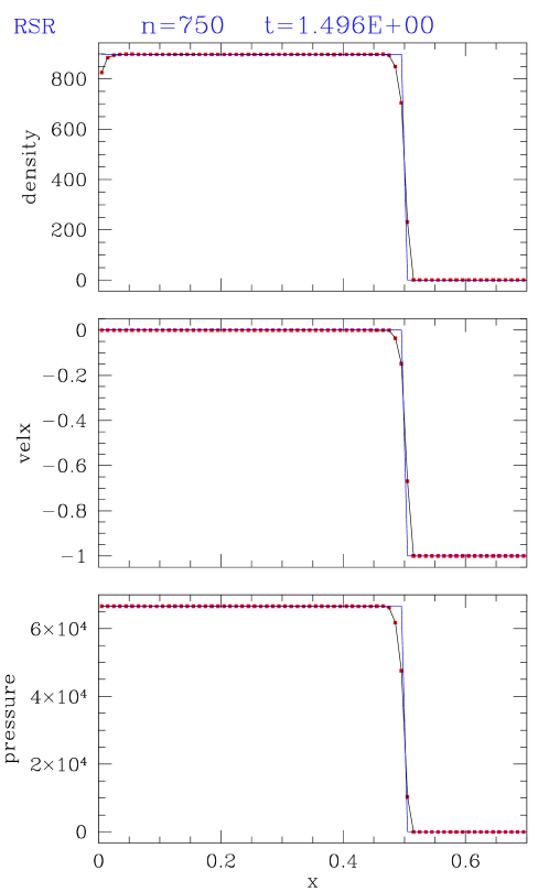
Figure 4: MPEG movie (only final frame of movie is displayed!) showing the evolution of the density distribution for the shock heating problem with an inflow velocity $v_{1}=-0.99999c$ in Cartesian coordinates. The reflecting wall is located at $x=0$. The adiabatic index of the gas is 4/3. For numerical reasons, the specific internal energy of the inflowing cold gas is set to a small finite value ($\varepsilon_{1}=10^{-7}\,W_{1}$). The final frame of the movie also shows the analytical solution (blue lines). The simulation has been performed on an equidistant grid of 100 zones.

The performance of a HRSC method based on a relativistic Riemann solver is illustrated by means of a MPEG movie (final frame of movie is displayed in Fig. 4) for the planar shock heating problem for an inflow velocity $v_{1}=-0.99999c$ ($W_{1}\approx 223$). These results are obtained with the relativistic PPM code of [106], which uses an exact Riemann solver based on the procedure described in Section 2.3.

The shock wave is resolved by three zones and there are no post–shock numerical oscillations. The density increases by a factor $\approx 900$ across the shock. Near $x=0$ the density distribution slightly undershoots the analytical solution (by $\approx 8\%$) due to the numerical effect of wall heating. The profiles obtained for other inflow velocities are qualitatively similar. The mean relative error of the compression ratio $\sigma_{\rm error}<10^{-3}$, and, in agreement with other codes based on a Riemann solver, the accuracy of the results does not exhibit any significant dependence on the Lorentz factor of the inflowing gas.

Some authors have considered the problem of shock heating in cylindrical or spherical geometry using adapted coordinates to test the numerical treatment of geometrical factors [153, 108, 182]. Aloy et al. [2] have considered the spherically symmetric shock heating problem in 3D Cartesian coordinates as a test case for both the directional splitting and the symmetry properties of their code GENESIS. The code is able to handle this test up to inflow Lorentz factors of the order of 700.

In the shock reflection test conventional schemes often give numerical approximations which exhibit a consistent $O(1)$ error for the density and internal energy in a few cells near the reflecting wall. This ’overheating’, as it is known in classical hydrodynamics [127], is a numerical artifact which is considerably reduced when Marquina’s scheme is used [42].

6.2 Propagation of relativistic blast waves

Riemann problems with large initial pressure jumps produce blast waves with dense shells of material propagating at relativistic speeds (see Fig. 5). For appropriate initial conditions, both the speed of the leading shock front and the velocity of the shell material approach the speed of light producing very narrow structures. The accurate description of these thin, relativistic shells involving large density contrasts is a challenge for any numerical code. Some particular blast wave problems have become standard numerical tests. Here we consider the two most common of these tests. The initial conditions are given in Table 5.

Figure 5: Generation and propagation of a relativistic blast wave (schematic). The large pressure jump at a discontinuity initially located at $r=05$ gives rise to a blast wave and a dense shell of material propagating at relativistic speeds. For appropriate initial conditions both the speed of the leading shock front and the velocity of the shell approach the speed of light producing very narrow structures.

Table 5: Initial data (pressure $p$, density $\rho$, velocity $v$) for two common relativistic blast wave test problems. The decay of the initial discontinuity leads to a shock wave (velocity $v_{\rm shock}$, compression ratio $\sigma_{\rm shock}$) and the formation of a dense shell (velocity $v_{\rm shell}$, time–dependent width $w_{\rm shell}$) both propagating to the right. The gas is assumed to be ideal with an adiabatic index $\gamma=5/3$.

	Problem 1		Problem 2
	Left	Right	Left	Right
$p$	13.33	0.00	1000.00	0.01
$\rho$	10.00	1.00	1.00	1.00
$v$	0.00	0.00	0.00	0.00
$v_{\rm shell}$	0.72		0.960
$w_{\rm shell}$	0.11 $t$		0.026 $t$
$v_{\rm shock}$	0.83		0.986
$\sigma_{\rm shock}$	5.07		10.75

Problem 1 was a demanding problem for relativistic hydrodynamic codes in the mid eighties [27, 75], while Problem 2 is a challenge even for today’s state-of-the-art codes. The analytical solution of both problems can be obtained with program RIEMANN (see Sect. 9.3).

6.2.1 Problem 1

In Problem 1, the decay of the initial discontinuity gives rise to a dense shell of matter with velocity $v_{\rm shell}=0.72$ ($W_{\rm shell}=1.38$) propagating to the right. The shell trailing a shock wave of speed $v_{\rm shock}=0.83$ increases its width, $w_{\rm shell}$, according to $w_{\rm shell}=0.11t$, i.e., at time $t=0.4$ the shell covers about 4% of the grid ($0\leq x\leq 1$). Tables 6,7 give a summary of the references where this test was considered for non-HRSC and HRSC methods, respectively.

Table 6: Summary of references where the blast wave Problem 1 (defined in Table 5) has been considered in 1D, 2D and 3D, respectively. Methods are described in Sects. 3 and 4 and their basic properties summarized in Sect. 5 (Tables 2,3).

References	Dim.	Method	Comments
Centrella & Wilson (1984) [27]	1D	AV-mono	Stable profiles without oscillations
			Velocity overestimated by $7\%$
Hawley et al. (1984) [75]	1D	AV-mono	Stable profiles without oscillations
			$\rho_{\rm shell}$ overestimated by $16\%$
Dubal (1991)a [44]	1D	FCT-lw	10-12 zones at the CD
			Velocity overestimated by 4.5%
Mann (1991) [99]	1D	SPH-AV-0,1,2	Sistematic errors in the rarefaction
			wave and the constant states
			Large amplitud spikes at the CD
			Excessive smearing at the shell
Laguna et al. (1993) [88]	1D	SPH-AV-0	Large amplitud spikes at the CD
			$\rho_{\rm shell}$ overestimated by $5\%$
van Putten (1993)b [175]	1D	van Putten	Stable profiles
			Excessive smearing, specially at the
			CD ($\approx 50$ zones)
Schneider et al. (1993) [157]	1D	SHASTA-c	Non monotonic intermediate states
			$\rho_{\rm shell}$ underestimated by $10\%$ with
			200 zones
Chow & Monaghan (1997) [29]	1D	SPH-RS-c	Stable profiles without spikes
			Excessive smearing at the CD and
			at the shock
Siegler & Riffert (1999) [160]	1D	SPH-cAV-c	Correct constant states
			Large amplitud spikes at the CD
			Excessive smearing at the shock
			transition ($\approx 20$ zones)

^a For a Riemann problem with slightly different initial conditions.
^b For a Riemann problem with slightly different initial conditions including a nonzero transverse magnetic field.

Table 7: Summary of references where the blast wave Problem 1 (defined in Table 5) has been considered in 1D, 2D and 3D, respectively. Methods are described in Sects. 3 and 4 and their basic properties summarized in Sect. 5 (Tables 2,3).

References	Dim.	Method	Commentsa
Eulderink (1993) [50]	1D	Roe-Eulderink	Correct $\rho_{\rm shell}$ with 500 zones
			4 zones at the CD
Schneider et al. (1993) [157]	1D	HLL-l	$\rho_{\rm shell}$ underestimated by $10\%$
			with 200 zones
Martí & Müller (1996) [106]	1D	rPPM	Correct $\rho_{\rm shell}$ with 400 zones
			6 zones at the CD
Martí et al. (1997) [108]	1D, 2D	MFF-ppm	Correct $\rho_{\rm shell}$ with 400 zones
			6 zones at the CD
Wen et al. (1997) [182]	1D	rGlimm	No difussion at discontinuities
Yang et al. (1997) [191]	1D	rBS	Stable profiles
Donat et al. (1998) [42]	1D	MFF-eno	Correct $\rho_{\rm shell}$ with 400 zones
			8 zones at the CD
Aloy et al. (1999) [2]	3D	MFF-ppm
Font et al. (1999) [59]	1D, 3D	MFF-l	Correct $\rho_{\rm shell}$ with 400 zones
			12-14 zones at the CD
	1D, 3D	Roe type-l	Correct $\rho_{\rm shell}$ with 400 zones
			12-14 zones at the CD
	1D, 3D	Flux split	$\rho_{\rm shell}$ overestimated by $5\%$
			8 zones at the CD

^a All the methods produce stable profiles without numerical oscillations. Comments correspond to 1D cases.

Using artificial viscosity techniques Centrella & Wilson [27] were able to reproduce the analytical solution with a 7% overshoot in $v_{\rm shell}$, whereas Hawley et al. [75] got a 16% error in the shell density.

The results obtained with early relativistic SPH codes [99] were affected by systematic errors in the rarefaction wave and the constant states, large amplitud spikes at the contact discontinuity and large smearing. Smaller systematic errors and spikes are obtained with Laguna et al. ’s (1993) code [88]. This code also leads to a large overshoot in the shell’s density. Much cleaner states are obtained with the methods of Chow & Monaghan (1997) [29] and Siegler & Riffert (1999) [160], both based on conservative formulations of the SPH equations. In the case of Chow & Monaghan’s (1997) method [29], the spikes at the contact discontinuity dissapear but at the cost of an excessive smearing. Shock profiles with relativistic SPH codes are more smeared out than with HRSC methods covering typically more than 10 zones.

Van Putten has considered a similar initial value problem with somewhat more extreme conditions ($v_{\rm shell}\approx 0.82c$, $\sigma_{\rm shock}\approx 5.1$) and with a transversal magnetic field. For suitable choices of the smoothing parameters his results are accurate and stable, although discontinuities appear to be more smeared than with typical HRSC methods (6–7 zones for the strong shock wave; $\approx 50$ zones for the contact discontinuity).

MPEG movie 2 (final frame of movie is displayed in Fig. 6) shows the Problem 1 blast wave evolution obtained with a modern HRSC method (the relativistic PPM method introduced in Section 3.1). The grid has 400 equidistant zones, and the relativistic shell is resolved by 16 zones. Because of both the high order accuracy of the method in smooth regions and its small numerical diffusion (the shock is resolved with 4–5 zones only) the density of the shell is accurately computed (errors less than 0.1%). Other codes based on relativistic Riemann solvers [51] give similar results (see Table 7). The relativistic HLL method [157] underestimates the density in the shell by about 10% in a 200 zone calculation.

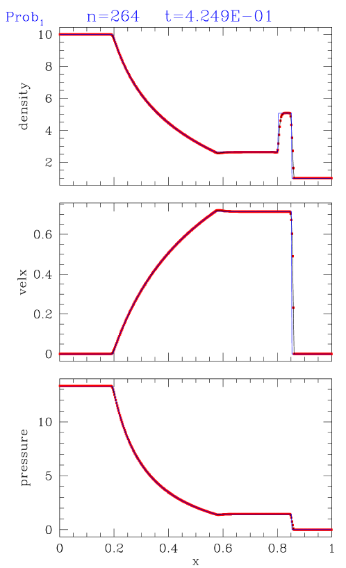
Figure 6: MPEG movie (only final frame of movie is displayed!) showing the evolution of the density distribution for the relativistic blast wave Problem 1 defined in Table 5. The final frame of the movie also shows the analytical solution (blue lines). The simulation has been performed with relativistic PPM on an equidistant grid of 400 zones.

6.2.2 Problem 2

Problem 2 was first considered by Norman & Winkler[128]. The flow pattern is similar to that of Problem 1, but more extreme. Relativistic effects reduce the post–shock state to a thin dense shell with a width of only about 1% of the grid length at $t=0.4$. The fluid in the shell moves with $v_{\rm shell}=0.960$ (i.e., $W_{\rm shell}=3.6$), while the leading shock front propagates with a velocity $v_{\rm shock}=0.986$ (i.e., $W_{\rm shock}=6.0$). The jump in density in the shell reaches a value of 10.6. Norman & Winkler [128] obtained very good results with an adaptive grid of 400 zones using an implicit hydro–code with artificial viscosity. Their adaptive grid algorithm placed 140 zones of the available 400 zones within the blast wave thereby accurately capturing all features of the solution.

Several HRSC methods based on relativistic Riemann solvers have used Problem 2 as a standard test [104, 103, 106, 55, 182, 42] (see Table 8).

Table 8: Summary of references where the blast wave Problem 2 (defined in Table 5) has been considered. Methods are described in Sects. 3 and 4 and their basic properties summarized in Sect. 5 (Tables 2,3).

References	Method	$\sigma/\sigma_{\rm exact}$
Norman & Winkler (1986) [128]	cAV-implicit	1.00
Dubal (1991) [44]a	FCT-lw	0.80
Martí et al. (1991) [104]	Roe type-l	0.53
Marquina et al. (1992) [103]	LCA-phm	0.64
Martí & Müller (1996) [106]	rPPM	0.68
Falle & Komissarov (1996) [55]	Falle-Komissarov	0.47
Wen et al. (1997) [182]	rGlimm	1.00
Chow & Monaghan (1997) [29]	SPH-RS-c	1.16b
Donat et al. (1998) [42]	MFF-phm	0.60

^a For a Riemann problem with slightly different initial conditions.
^b At $t=0.15$.

MPEG movie 3 (final frame of movie is displayed in Fig. 7) shows the Problem 2 blast wave evolution obtained with the relativistic PPM method introduced in Section 3.1) on a grid of 2000 equidistant zones. At this resolution the relativistic PPM code obtains a converged solution. The method of Falle & Komissarov [55] requires a seven–level adaptive grid calculation to achieve the same the finest grid spacing corresponding to a grid of 3200 zones. As their code is free of numerical diffusion and dispersion, Wen et al. [182] are able to handle this problem with high accuracy (see Fig 8). At lower resolution (400 zones) the relativistic PPM method only reaches 69% of the theoretical shock compression value (54% in case of the second–order accurate upwind method of Falle & Komissarov [55]; 60% with the code of Donat et al. [42]).

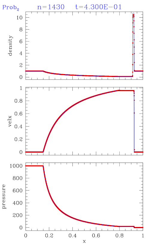
Figure 7: MPEG movie (only final frame of movie is displayed!) showing the evolution of the density distribution for the relativistic blast wave Problem 2 defined in Table 5. The final frame of the movie also shows the analytical solution (blue lines). The simulation has been performed with relativistic PPM on an equidistant grid of 2000 zones.

Figure 8: Results from [182] for the relativistic blast wave Problems 1 (left column) and 2 (right column), respectively. Relativistic Glimm’s method is only used in regions with steep gradients. Standard finite difference schemes are applied in the smooth remaining part of the computational domain. In the above plots, Lax and LW stand respectively for Lax and Lax-Wendroff methods; G refers to pure Glimm’s method.

Chow & Monaghan [29] have considered Problem 2 to test their relativistic SPH code. Besides a 15% overshoot in the shell’s density, the code produces a non–causal blast wave propagation speed (i.e., $v_{\rm shock}>1$).

6.2.3 Collision of two relativistic blast waves

The collision of two strong blast waves was used by Woodward & Colella [186] to compare the performance of several numerical methods in classical hydrodynamics. In the relativistic case, Yang et al. [191] considered this problem to test the high-order extensions of the relativistic beam scheme, whereas Martí & Müller [106] used it to evaluate the performance of their relativistic PPM code. In this last case, the original boundary conditions were changed (from reflecting to outflow) to avoid the reflection and subsequent interaction of rarefaction waves allowing for a comparison with an analytical solution. In the following we summarize the results on this test obtained by Martí & Müller in [106].

The initial data corresponding to this test, consisting in three constant states with large pressure jumps at the discontinuities separating the states (at $x=0.1$ and $x=0.9$), as well as the properties of the blast waves created by the decay of the initial discontinuities, are listed in Table 9. The propagation velocity of the two blast waves is slower than in the Newtonian case, but very close to the speed of light (0.9776 and $-0.9274$ for the shock wave propagating to the right and left, respectively). Hence, the shock interaction occurs later (at $t=0.420$) than in the Newtonian problem (at $t=0.028$). Top panel in Fig. 9 shows four snapshots of the density distribution including the moment of the collision of the blast waves at $t=0.420$ and $x=0.5106$. At the time of collision the two shells have a width of $\Delta x=0.008$ (left shell) and $\Delta x=0.019$ (right shell), respectively, i.e., the whole interaction takes place in a very thin region (about 10 times smaller than in the Newtonian case where $\Delta x\approx 0.2$).

Table 9: Initial data (pressure $p$, density $\rho$, velocity $v$) for the two relativistic blast wave collision test problem. The decay of the initial discontinuities (at $x=0.1$ and $x=0.9$) leads to the formation of two shock waves (velocities $v_{\rm shock}$, compression ratios $\sigma_{\rm shock}$) leading two dense shells (velocities $v_{\rm shell}$, time–dependent widths $w_{\rm shell}$) moving in opposite directions. The gas is assumed to be ideal with an adiabatic index $\gamma=1.4$.

	Left	Middle		Right
$p$	1000.00	0.01		100.00
$\rho$	1.00	1.00		1.00
$v$	0.00	0.00		0.00
$v_{\rm shell}$	0.957		$-$0.882
$w_{\rm shell}$	0.021 $t$		0.045 $t$
$v_{\rm shock}$	0.978		$-$0.927
$\sigma_{\rm shock}$	14.39		9.72

Figure 9: The top panel shows a sequence of snapshots of the density profile for the colliding relativistic blast wave problem up to the moment when the waves begin to interact. The density profile of the new states produced by the interaction of the two waves is shown in the bottom panel (note the change in scale on both axes with respect to the top panel).

The collision gives rise to a narrow region of very high density (see lower panel of Fig. 9) bounded by two shocks moving at speeds 0.088 (shock at the left) and 0.703 (shock at the right) and large compression ratios (7.26 and 12.06, respectively) well above the classical limit for strong shocks (6.0 for $\gamma=1.4$). The solution just described applies until $t=0.430$ when the next interaction takes place.

The complete analytical solution before and after the collision up to time $t=0.430$ can be obtained following Appendix II in [106].

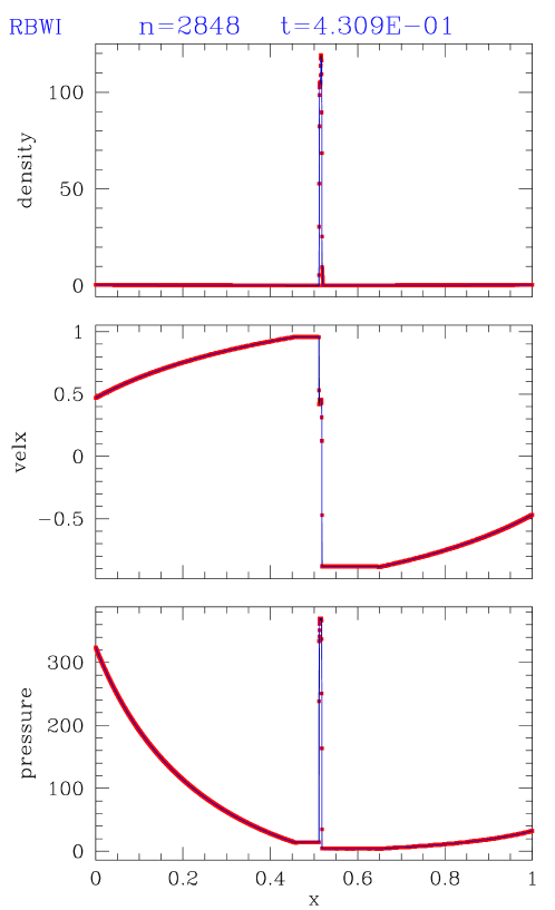
Figure 10: MPEG movie (only final frame of movie is displayed!) showing the evolution of the density distribution for the colliding relativistic blast wave problem up to the interaction of the waves. The final frame of the movie also shows the analytical solution (blue lines). The computation has been performed with relativistic PPM on an equidistant grid of 4000 zones.

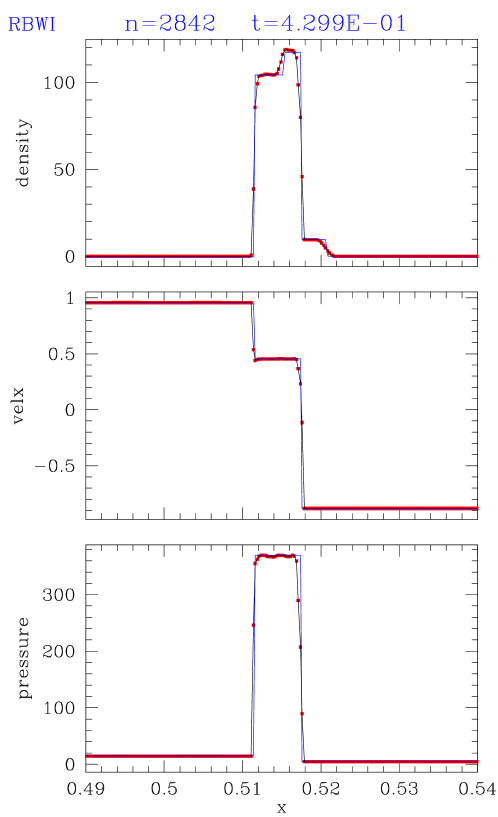
Figure 11: MPEG movie (only final frame of movie is displayed!) showing the evolution of the density distribution for the colliding relativistic blast wave problem around the time of interaction of the waves at an enlarged spatial scale. The final frame of the movie also shows the analytical solution (blue lines). The computation has been performed with relativistic PPM on an equidistant grid of 4000 zones.

MPEG movie 4 (final frame of movie is displayed in Fig. 10) shows the evolution of the density up to the time of shock collision at $t=0.4200$. The movie was obtained with the relativistic PPM code of Martí & Müller [106]. The presence of very narrow structures involving large density jumps requires very fine zoning to resolve the states properly. For the movie a grid of 4000 equidistant zones was used. The relative error in the density of the left (right) shell is always less than $2.0\%$ ($0.6\%$), and is about $1.0\%$ ($0.5\%$) at the moment of shock collision. Profiles obtained with the relativistic Godunov method (first–order accurate, not shown) show relative errors in the density of the left (right) shell of about $50\%$ ($16\%$) at $t=0.20$. The errors drop only slightly to about $40\%$ ($5\%$) at the time of collision ($t=0.420$).

MPEG movie 5 (final frame of movie is displayed in Fig. 11) shows the numerical solution after the interaction has occurred. Compared to MPEG movie 4 (final frame of movie is displayed in Fig.  10) a very different scaling for the x-axis had to be used to display the narrow dense new states produced by the interaction. Obviously, the relativistic PPM code resolves the structure of the collision region satisfactorily well, the maximum relative error in the density distribution being less than $2.0\%$. When using the first–order accurate Godunov method instead, the new states are strongly smeared out and the positions of the leading shocks are wrong.

7 APPLICATIONS

7.1 Astrophysical jets

The most compelling case for a special relativistic phenomenon are the ubiquitous jets in extragalactic radio sources associated with active galactic nuclei. In the commonly accepted standard model [10], flow velocities as large as 99% (in some cases even beyond) of the speed of light are required to explain the apparent superluminal motion observed in many of these sources. Models which have been proposed to explain the formation of relativistic jets, involve accretion onto a compact central object, such as a neutron star or stellar mass black hole in the galactic micro–quasars GRS 1915+105 [116] and GRO J1655-40 [169], or a rotating super massive black hole in an active galactic nucleus, which is fed by interstellar gas and gas from tidally disrupted stars.

Inferred jet velocities close to the speed of light suggest that jets are formed within a few gravitational radii of the event horizon of the black hole. Moreover, very–long–baseline interferometric (VLBI) radio observations reveal that jets are already collimated at subparsec scales. Current theoretical models assume that accretion disks are the source of the bipolar outflows which are further collimated and accelerated via MHD processes (see, e.g., [15]). There is a large number of parameters which are potentially important for jet powering: the black hole mass and spin, the accretion rate and the type of accretion disk, the properties of the magnetic field and of the environment.

At parsec scales the jets, observed via their synchrotron and inverse Compton emission at radio frequencies with VLBI imaging, appear to be highly collimated with a bright spot (the core) at one end of the jet and a series of components which separate from the core, sometimes at superluminal speeds. In the standard model [16], these speeds are interpreted as a consequence of relativistic bulk motions in jets propagating at small angles to the line of sight with Lorentz factors up to 20 or more. Moving components in these jets, usually preceded by outbursts in emission at radio wavelengths, are interpreted in terms of traveling shock waves.

Finally, the morphology and dynamics of jets at kiloparsec scales are dominated by the interaction of the jet with the surrounding extragalactic medium, the jet power being responsible for dichotomic morphologies (the so called Fanaroff–Riley I and II classes [56], FR I and FR II, respectively). Whereas current models [13, 90] interpret FR I morphologies as the result of a smooth deceleration from relativistic to non–relativistic, transonic speeds on kpc scales due to a slower shear layer, flux asymmetries between jets and counter–jets in the most powerful radio galaxies (FRII) and quasars indicate that relativistic motion extends up to kpc scales in these sources, although with smaller values of the overall bulk speeds [20].

Although MHD and general relativistic effects seem to be crucial for a successful launch of the jet (for a review see, e.g., [22]), purely hydrodynamic, special relativistic simulations are adequate to study the morphology and dynamics of relativistic jets at distances sufficiently far from the central compact object (i.e., at parsec scales and beyond). The development of relativistic hydrodynamic codes based on HRSC techniques (see Sections 3 and 4) has triggered the numerical simulation of relativistic jets at parsec and kiloparsec scales.

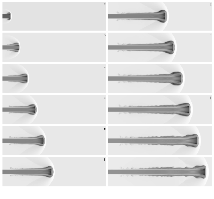
Figure 12: Time evolution of a light, relativistic (beam flow velocity equal to 0.99) jet with large internal energy. The logarithm of the proper rest–mass density is plotted in grey scale the maximum value corresponding to white and the minimum to black.

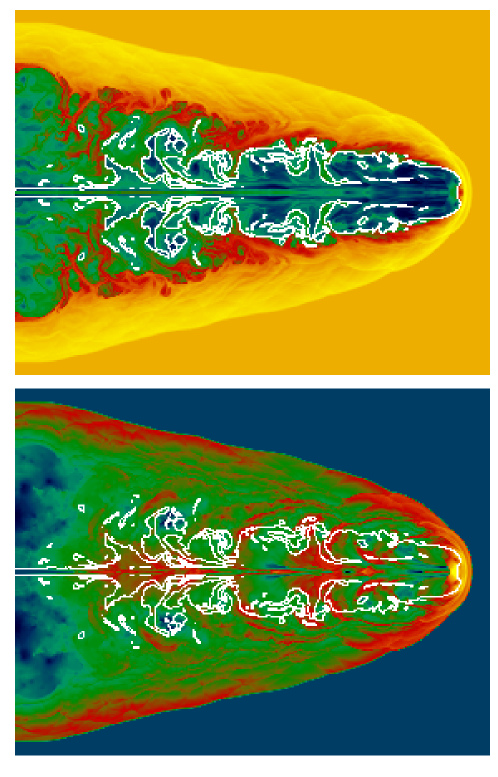
Figure 13: Logarithm of the proper rest–mass density and energy density (from top to bottom) of an evolved, powerful jet propagating through the intergalactic medium. The white contour encompasses the jet material responsible for the synchrotron emission.

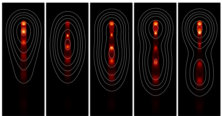
Figure 14: Computed radio maps of a compact relativistic jet showing the evolution of a superluminal component (from left to right). Two resolutions are shown: present VLBI resolution (white contours) and resolution provided by the simulation (black/white images).

At kiloparsec scales, the implications of relativistic flow speeds and/or relativistic internal energies for the morphology and dynamics of jets have been the subject of a number of papers in recent years [109, 46, 107, 108, 85]. Beams with large internal energies show little internal structure and relatively smooth cocoons allowing the terminal shock (the hot spot in the radio maps) to remain well defined during the evolution. Their morphologies resemble those observed in naked quasar jets like 3C273 [36]. Fig. 12 shows several snapshots of the time evolution of a light, relativistic jet with large internal energy. The dependence of the beam’s internal structure on the flow speed suggests that relativistic effects may be relevant for the understanding of the difference between slower, knotty BL Lac jets and faster, smoother quasar jets [60].

Highly supersonic models, in which kinematic relativistic effects due to high beam Lorentz factors dominate, have extended overpressured cocoons. These overpressured cocoons can help to confine the jets during the early stages of their evolution [107] and even cause their deflection when propagating through non–homogeneous environments [145]. The cocoon overpressure causes the formation of a series of oblique shocks within the beam in which the synchrotron emission is enhanced. In long term simulations (see Fig. 13), the evolution is dominated by a strong deceleration phase during which large lobes of jet material (like the ones observed in many FR IIs, e.g., Cyg A [24]) start to inflate around the jet’s head. These simulations reproduce some properties observed in powerful extragalactic radio jets (lobe inflation, hot spot advance speeds and pressures, deceleration of the beam flow along the jet) and can help to constrain the values of basic parameters (such as the particle density and the flow speed) in the jets of real sources.

The development of multidimensional relativistic hydrodynamic codes has allowed, for the first time, the simulation of parsec scale jets and superluminal radio components [68, 84, 115]. The presence of emitting flows at almost the speed of light enhances the importance of relativistic effects in the appearance of these sources (relativistic Doppler boosting, light aberration, time delays). Hence, one should use models which combine hydrodynamics and synchrotron radiation transfer when comparing with observations. In these models, moving radio components are obtained from perturbations in steady relativistic jets. Where pressure mismatches exist between the jet and the surrounding atmosphere reconfinement shocks are produced. The energy density enhancement produced downstream from these shocks can give rise to stationary radio knots as observed in many VLBI sources. Superluminal components are produced by triggering small perturbations in these steady jets which propagate at almost the jet flow speed. One example of this is shown in Fig. 14 (see also [68]), where a superluminal component (apparent speed $\approx 7$ times the speed of light) is produced from a small variation of the beam flow Lorentz factor at the jet inlet. The dynamic interaction between the induced traveling shocks and the underlying steady jet can account for the complex behavior observed in many sources [67].

The first magnetohydrodynamic simulations of relativistic jets have been already undertaken in 2D [81, 80] and 3D [125, 126] to study the implications of ambient magnetic fields in the morphology and bending properties of relativistic jets. However, despite the impact of these results in specific problems like ,e.g., , the understanding of the misalignement of jets between pc and kpc scales, these 3D simulations have not addressed the effects on the jet structure and dynamics of the third spatial degree of freedom. This has been the aim of the work undertaken by Aloy et al. [3].

Finally, Koide et al. [82] have developed a general relativistic MHD code and applied it to the problem of jet formation from black hole accretion disks. Jets are formed with a two-layered shell structure consisting of a fast gas pressure driven jet (Lorentz factor $\approx 2$) in the inner part and a slow magnetically driven outflow in the outer part both of which being collimated by the global poloidal magnetic field penetrating the disk.

7.2 Gamma-Ray Bursts (GRBs)

A second phenomenon which involves flows with velocities very close to the speed of light are gamma-ray bursts (GRBs). Although known observationally since over 30 years, until recently their distance (“local” or “cosmological”) has been, and their nature still is a matter of controversial debate [57, 112, 140, 141]. GRBs do not repeat except for a few soft gamma–ray repeaters. They are detected with a rate of about one event per day, and their duration varies from milliseconds to minutes. The duration of the shorter bursts and the temporal substructure of the longer bursts implies a geometrically small source (less than $\sim c\cdot 1{\rm msec}\sim 100\,$km), which in turn points towards compact objects, like neutron stars or black holes. The emitted gamma–rays have energies in the range 30 keV to 2 MeV.

Concerning the distance of GRB sources major progress has occured through the observations by the BATSE detector on board the Compton Gamma–Ray Observatory (GRO), which have proven that GRBs are distributed isotropically over the sky [111]. Even more important the detection and the rapid availability of accurate coordinates ($\sim$ arc minutes) of the fading X–ray counterparts of GRBs by the BeppoSAX spacecraft beginning in 1997 [33, 143] has allowed for subsequent successful ground based observations of faint GRB afterglows at optical and radio wavelength. In case of GRB 990123 the optical, X–ray and gamma–ray emission was detected for the first time almost simultaneously (optical observations began 22 seconds after the onset of the GRB) [21, 1]. From optical spectra thus obtained redshifts of several gamma–ray bursts have been determined, e.g., GRB 970508 ($z=0.835$ [113, 137]), GRB 971214 ($z=3.42$ [86]), GRB 980703 ($z=0.966$ [40]) and GRB 990123 ($1.60\leq z<2.05$ [5]), which confirm that (at least some) GRBs occur at cosmological distances. Assuming isotropic emission the inferred total energy of cosmological GRBs emitted in form of gamma–rays ranges from several $10^{51}\,$erg to $3\,10^{53}\,$erg (for GRB 971214) [25], and exceeds $10^{54}\,$erg for GRB 990123 [5, 21]. Updated information on GRBs localized with BeppoSAX, BATSE/RXTE(PCA) or BATSE/RXTE(ASM) can be obtained from a web site maintained by Greiner [71].

The compact nature of the GRB source, the observed flux and the cosmological distance taken together imply a large photon density. Such a source has a large optical depth for pair production. This is, however, inconsistent with the optically thin source indicated by the non–thermal gamma–ray spectrum, which extends well beyond the pair production threshold at 500 keV. This problem can be resolved by assuming an ultra-relativistic expansion of the emitting region, which eliminates the compactness constraint. The bulk Lorentz factor required are then $W>100$ (see, e.g., [141])

In April 1998 the pure cosmological origin of GRBs was challenged by the detection of the Type Ib/c supernova SN 1998bw [61, 62] within the 8 arc minute error box of GRB 980425 [161, 138]. Its explosion time is consistent with that of the GRB, and relativistic expansion velocities are derived from radio observations of SN 1998bw [87]. BeppoSAX detected two fading X–ray sources within the error box, one being positionally consistent with the supernova and a fainter one not consistent with the position of SN 1998bw [138]. Taken together these facts suggest a relationship between GRBs and SNe Ib/c, i.e., core collapse supernovae of massive stellar progenitors which have lost their hydrogen and helium envelopes [62, 78, 188]. As the host galaxy ESO 184-82 of SN 1998bw is only at a redshift of $z=0.0085$ [170] and as GRB 980425 was not extraordinarily bright, GRB–supernovae are more than four orders of magnitude fainter ($E{\rm tot}_{\gamma}=7\,10^{47}\,$erg for GRB 980425 [25]) than a typical cosmological GRB. However, the observation of the second fading X–ray source within the error box of GRB 980425 and unrelated with SN 1998bw still causes some doubts on the GRB supernova connection, although the probability of chance coincidence of GRB 980425 and SN 1998bw is extremely low [138].

In order to explain the energies released in a GRB various catastrophic collapse events have been proposed including neutron–star/neutron–star mergers [131, 69, 48], neutron–star/black–hole mergers [117], collapsars [187, 98] and hypernovae [132]. These models all rely on a common engine, namely a stellar mass black hole which accretes several solar masses of matter from a disk (formed during a merger or by a non–spherical collapse) at a rate of $\sim 1\,M_{\odot}\,$s^-1 [147]. A fraction of the gravitational binding energy released by accretion is converted into neutrino and anti–neutrino pairs, which in turn annihilate into electron–positron pairs. This creates a pair fireball, which will also include baryons present in the environment surrounding the black hole. Provided the baryon load of the fireball is not too large, the baryons are accelerated together with the e${}^{+}\,$e^- pairs to ultra-relativistic speeds with Lorentz factors $>10^{2}$ [26, 142, 141]. The existence of such relativistic flows is supported by radio observations of GRB 980425 [87]. It has been further argued that the rapid temporal decay of several GRB afterglows is inconsistent with spherical (isotropic) blast wave models, and instead is more consistent with the evolution of a relativistic jet after it slows down and spreads laterally [156]. Independent of the flow pattern the bulk kinetic energy of the fireball then is thought to be converted into gamma-rays via cyclotron radiation and/or inverse Compton processes (see, e.g., [112, 141]).

One–dimensional numerical simulations of spherically symmetric relativistic fireballs have been performed by several authors to model GRB sources [142, 133, 134]. Multi-dimensional modelling of ultra–relativistic jets in the context of GRBs has for the first time been attempted by Aloy et al. [4]. Using a collapsar progenitor model of MacFadyen & Woosley [98] they have simulated the propagation of an axisymmetric jet through the mantle and envelope of a collapsing massive star ($10\,M_{\odot}$) using the GENESIS special relativistic hydrodynamic code [2]. The jet forms as a consequence of an assumed energy deposition of $10^{51}\,$erg/sec within a 30 degree cone around the rotation axis. At break-out, i.e., when the jets reaches the surface of the stellar progenitor, the maximum Lorentz factor of the jet flow is about 20.

8 CONCLUSION

8.1 Evaluation of the methods

An assessment of the quality of the numerical methods should consider, at least, the following aspects: (i) accuracy and robustness in describing high Lorentz factor flows with strong shocks; (ii) effort required to extend to multi dimensions; (iii) effort required to extend to RMHD and GRHD. In Table (10) we have summarized these aspects of numerical methods for SRHD.

Since their introduction in numerical RHD at the beginning of nineties, HRSC methods have demonstrated their ability to describe accurately (stable and without excessive smearing) relativistic flows of arbitrarily large Lorentz factors and strong discontinuities reaching the same quality as in classical hydrodynamics. In addition (as it is the case for classical flows, too), HRSC methods show the best performance compared to any other method (e.g., artificial viscosity, FCT or SPH).

Despite of the latter fact, a lot of effort has been put into improving these non HRSC methods. Using a consistent formulation of artificial viscosity has significantly enhanced the capability of finite difference schemes [128] as well as of relativistic SPH [160] to handle strong shocks without spurious post–shock oscillations. However, this comes at the price of a large numerical dissipation at shocks. Concerning relativistic SPH recent investigations using a conservative formulation of the hydrodynamic equations [29, 160] have reached an unprecedented accuracy with respect to previous simulations, although some issues still remain. Besides the strong smearing of shocks, the description of contact discontinuities and of thin structures moving at ultrarelativistic speeds needs to be improved (see Sect. 6.2).

Concerning FCT techniques, those codes based on a conservative formulation of the RHD equations have been able to handle relativistic flows with discontinuities at all flow speeds, although the quality of the results is below that of HRSC methods in all cases [157].

The extension to multi dimensions is simple for most relativistic codes. Finite difference techniques are easily extended using directional splitting. Note, however, that HRSC methods based on exact solutions of the Riemann problem [106, 182] first require the development of a multidimensional version of the relativistic Riemann solver. The adapting–grid, artificial viscosity, implicit code of Norman & Winkler [128] and the relativistic Glimm method of Wen et al. [182] are restricted to one dimensional flows. Note that Glimm’s method produces the best results in all the tests analyzed in Sect. 6.

The symmetric TVD scheme proposed by Davis [37] and extended to GRMHD (see below) by Koide et al. [81] combines several characteristics making it very attractive. It is written in conservation form and is TVD, i.e., it is converging to the physical solution. In addition, it is independent of spectral decompositions, which allows for a simple extension to RMHD. Quite similar statements can be made about the approach proposed by van Putten [175]. In contrast to FCT schemes (which are also easily extended to general systems of equations), both Koide et al. ’s and van Putten’s method are very stable when simulating mildly relativistic flows (maximum Lorentz factors $\approx 4$) with discontinuities. Their only drawback is an excessive smearing of the latter. A comparison of Davis’ method with Riemann solver based methods would be desirable.

Table 10: Evaluation of numerical methods for SRHD. Methods have been categorized for clarity

Method	Ultrarelativistic	Handling of	Extension to several	Extension to
	regime	discontinuities a	spatial dimensions b	GRHD	RMHD
AV-mono	$\times$	O, SE	$\surd$	$\surd$	$\times$
cAV-implicit	$\surd$	$\surd$	$\times$	$\times$	$\times$
HRSC c	$\surd$	$\surd$	$\surd$ d	$\surd$ e	$\times$ f
rGlimm	$\surd$	$\surd$	$\times$	$\times$	$\times$
sTVD	$\surd$ g	D	$\surd$	$\surd$	$\surd$
van Putten	$\surd$ g	D	$\surd$	$\times$	$\surd$
FCT	$\surd$	O	$\surd$	$\times$	$\times$
SPH	$\surd$	D, O	$\surd$	$\surd$ h	$\times$ i

^a D: excessive dissipation; O: oscillations; SE: systematic errors.
^b all finite difference methods are extended by directional splitting.
^c contains all the methods listed in Table 2 with exception of rGlimm [182] and sTVD [81].
^d rPPM [106] requires an exact relativistic Riemann solver with non-zero transverse speeds.
^e there exist GRHD extensions of several HRSC methods based on linearized Riemann solvers. The procedure developed by Pons et al. [146] allows any SRHD Riemann solver to be applied to GRHD flows.
^f except HLL which requires spectral decomposition of RMHD equations or solution of RMHD Riemann problem. Van Putten [180] has studied the characteristic structure of the RMHD equations in (constraint free) divergence form as a first step to extend modern HRSC methods to RMHD. Komissarov [83] has developed a multidimensional RMHD code based on a linearized Riemann solver.
^g needs confirmation.
^h codes of refs. [88, 160].
ⁱ There is one code which considered such an extension [99], but the results are not completely satisfactory.

8.2 Further developments

The directions of future developments in this field of research are quite obvious. They can be divided into four main categories:

8.2.1 Incorporation of realistic microphysics

Up to now most astrophysical SRHD simulations have assumed matter whose thermodynamic properties can be described by an inviscid ideal equation of state with a constant adiabatic index. This simplification may have been appropriate in the first generation of SRHD simulations, but it clearly must be given up when aiming at a more realistic modelling of astrophysical jets, gamma–ray burst sources or accretion flows onto compact objects. For these phenomena a realistic equation of state should include contributions from radiation ($\gamma=4/3$ “fluid”), allow for the formation of electron–positron pairs at high temperatures, allow the ideal gas contributions to be arbitrarily degenerate and/or relativistic. Effects due to cooling, heat conduction, nuclear transmutations and viscosity may have to be considered, too. When simulating relativistic heavy ion collisions the use of a realistic equation of state is essential for an adequate description of the phenomenon. However, as these simulations have been performed with FCT based difference schemes (see, e.g., [162]), this poses no specific numerical problem. The simulation of flows obeying an elaborated microphysics with HRSC methods needs in some cases the extension of the present relativistic Riemann solvers to handle general equations of state. This is the case of the Roe-Eulderink method (extendable by the procedure developed in the classical case by Glaister [64]), and rPPM and rGlimm both relying on a exact solution of the Riemann problem for ideal gases with constant adiabatic exponent (which can also be extended following the procedure of Colella & Glaz [31] for classical hydrodynamics). We expect the second generation of SRHD codes being capable of treating general equations of state and various source/sink terms routinely.

8.2.2 Coupling of SRHD schemes with AMR

Modelling astrophysical phenomena often involves an enormous range of length scales and time scales to be covered in the simulations. In two and definitely in three spatial dimensions many such simulations cannot be performed with sufficient spatial resolution on a static equidistant or non–equidistant computational grid, but they will require dynamic, adaptive grids. In our opinion the most promising approach in this direction will be the coupling of SRHD solvers with the adaptive mesh refinement (AMR) techniques [12]. AMR automatically increases the grid resolution near flow discontinuities or in regions of large gradients (of the flow variables) until a prescribed accuracy of the difference approximation is achieved. A SRHD simulation of a relativistic jet based on a combined HLL–AMR scheme was performed by Duncan & Hughes [46]. Plewa et al. [145] have modelled the deflection of highly supersonic jets propagating through non–homogeneous environments using the HRSC scheme of Martí et al. [108] combined with the AMR implementation AMRA of Plewa [144]. Komissarov & Falle [84] have combined their numerical scheme with the adaptive grid code, Cobra, which has been developed by Mantis Numerics Ltd. for industrial applications [54], and which uses a hierarchy of grids with a constant refinement factor of two between subsequent grid levels.

8.2.3 General relativistic hydrodynamics (GRHD)

Up to now only very few attempts have been made to extend HRSC methods to GRHD and all of these have used linearized Riemann solvers [104, 51, 153, 9, 59]. In the most recent of these approaches Font et al. [59] have developed a 3D general relativistic HRSC hydrodynamic code where the matter equations are integrated in conservation form and fluxes are calculated with Marquina’s formula. A very interesting and powerful procedure has been proposed by Pons et al. [146], which allows one to exploit all the developments in the field of special relativistic Riemann solvers in general relativistic hydrodynamics. The procedure relies on a local change of coordinates at each zone interface such that the spacetime metric is locally flat. In that locally flat spacetime any special relativistic Riemann solver can be used to calculate the numerical fluxes, which are then transformed back. Finer grids and improved time advancing methods will be required in regions where large gradients or temporal variations of the gravitational field are encountered. The numerical implementation is simple and computationally inexpensive.

The characteristic formulations of the Einstein field equations are able to handle the long term numerical description of single black hole space times in vacuum [14]. In order to include matter in such an scenario, Papadopoulos & Font [135] have generalized HRSC methods to cope with the hydrodynamic equations in this null foliation.

Other developments in GRHD in the past included finite element methods for simulating spherically symmetric collapse in general relativity [101], general relativistic pseudo–spectral codes based on the (3+1) ADM formalism [7] for computing radial perturbations [70] and 3D gravitational collapse of neutron stars [18], and general relativistic SPH [99]. The potential of these methods for the future is unclear, as none of them is specifically appropriate for ultrarelativistic speeds and strong shock waves which are characteristic of most astrophysical applications.

Peitz & Appl [136] have addressed the difficult issue of non–ideal GRHD, which is of particular importance, e.g., for the simulation of accretion discs around compact objects, rotating relativistic fluid configurations, and the evolution of density fluctuations in the early universe. They have accounted for dissipative effects by applying the theory of extended causal thermodynamics, which eliminates the causality violating infinite signal speeds arising from the conventional Navier–Stokes equation. Peitz & Appl have not implemented their model numerically yet.

8.2.4 Relativistic magneto–hydrodynamics (RMHD)

The inclusion of magnetic effects is of great importance in many astrophysical flows. The formation and collimation process of (relativistic) jets most likely involves dynamically important magnetic fields and occurs in strong gravitational fields. The same is likely to be true for accretion discs around black holes. Magneto–relativistic effects even play a non negligible role in the formation of proto–stellar jets in regions close to the light cylinder [22]. Thus, relativistic MHD codes are a very desirable tool in astrophysics. The non-trivial task of developing such a kind of code is considerably simplified by the fact that because of the high conductivity of astrophysical plasmas one must only consider ideal RMHD in most applications.

Special relativistic 2D MHD test problems with Lorentz factors up to $\sim 3$ have been investigated by Dubal [44] with a code based on FCT tecniques (see Sect. 4). In a series of papers Koide and coworkers [81, 80, 125, 126, 82] have investigated relativistic magnetized jets using a symmetric TVD scheme (see Sect. 3). Koide, Nishikawa & Mutel [81] simulated a 2D RMHD slab jet, whereas Koide [80] investigated the effect of an oblique magnetic field on the propagation of a relativistic slab jet. Nishikawa et al. [125, 126] extended these simulations to 3D and considered the propagation of a relativistic jet with a Lorentz factor $W=4.56$ along an aligned and an oblique external magnetic field. The 2D and 3D simulations published up to now only cover the very early propagation of the jet (up to 20 jet radii) and are performed with moderate spatial resolution on an equidistant Cartesian grid (up to 101 zones per dimension, i.e., 5 zones per beam radius).

Van Putten [174, 175] has proposed a method for accurate and stable numerical simulations of RMHD in the presence of dynamically significant magnetic fields in two dimensions and up to moderate Lorentz factors. The method is based on MHD in divergence form using a 2D shock–capturing method in terms of a pseudo–spectral smoothing operator (see Sect. 4. He applied this method to 2D blast waves [177] and astrophysical jets [176, 179].

Steps towards the extension of linearized Riemann solvers to ideal RMHD have already been taken. Romero [154] has derived an analytical expression for the spectral decomposition of the Jacobian in the case of a planar relativistic flow field permeated by a transversal magnetic field (nonzero field component only orthogonal to flow direction). Van Putten [180] has studied the characteristic structure of the RMHD equations in (constraint free) divergence form. Finally, Komissarov [83] has presented a robust Godunov–type scheme for RMHD, which is based on a linear Riemann solver, has second–order accuracy in smooth regions, enforces magnetic flux conservation, and which can cope with ultrarelativistic flows.

We end with the simulations performed by Koide, Shibata & Kudoh [82] on magnetically driven axisymmetric jets from black hole accretion disks. Their GRMHD code is an extension of the special relativistic MHD code developed by Koide et al. [81, 80, 125]. The necessary modifications of the code were quite simple, because in the (nonrotating) black hole’s Schwarzschild spacetime the GRMHD equations are identical to the SRMHD equations in general coordinates, except for the gravitational force terms and the geometric factors of the lapse function. With the pioneering work of Koide, Shibata & Kudoh the epoch of exciting GRMHD simulations has just begun.

9 ADDITIONAL INFORMATION

9.1 Algorithms to recover primitive quantities

The expressions relating the primitive variables $(\rho,v^{i},p)$ to the conserved quantities $(D,S^{i},\tau)$ depend explicitly on the equation of state $p(\rho,\varepsilon)$ and simple expressions are only obtained for simple equations of state (i.e., ideal gas).

A function of pressure, whose zero represents the pressure in the physical state, can easily be obtained from Eqs. (8–10), (12) and (13):

$$f(\bar{p})=p\left(\rho_{\ast}(\bar{p}),\varepsilon_{\ast}(\bar{p})\right)-\bar{p}$$ (61)

with $\rho_{\ast}(\bar{p})$ and $\varepsilon_{\ast}(\bar{p})$ given by

$$\rho_{\ast}(\bar{p})=\frac{D}{W_{\ast}(\bar{p})}\,,$$ (62)

and

$$\varepsilon_{\ast}(\bar{p})=\frac{\tau+D\,[1-W_{\ast}(\bar{p})]+\bar{p}\,[1-W_{\ast}(\bar{p})^{2}])}{D\,W_{\ast}(\bar{p})}\,,$$ (63)

where

$$W_{\ast}(\bar{p})=\frac{1}{{\displaystyle\sqrt{1-v_{\ast}^{i}(\bar{p})v_{\ast\,i}(\bar{p})}}}\,$$ (64)

and

$$v_{\ast}^{i}(\bar{p})=\frac{S^{i}}{\tau+D+\bar{p}}\,.$$ (65)

The root of (61) can be obtained by means of a nonlinear root–finder (e.g., a one–dimensional Newton–Raphson iteration). For an ideal gases with a constant adiabatic exponent such a procedure has proven to be very successful in a large number of tests and applications [104, 106, 108]. The derivative of $f$ with respect to $\bar{p}$, $f^{\prime}$, can be approximated by [2]

$$f^{\prime}=v_{\ast}^{i}(\bar{p})v_{\ast\,i}(\bar{p})c_{s\,\ast}(\bar{p})^{2}-1\,,$$ (66)

where $c_{s\ast}$ is the sound speed which can efficiently be computed for any EOS. Moreover, approximation (66) tends to the exact derivative as the solution is approached.

Eulderink [50, 51] has also developed several procedures to calculate the primitive variables for an ideal EOS with a constant adiabatic index. One procedure is based on finding the physically admissible root of a fourth–order polynomial of a function of the specific enthalpy. This quartic equation can be solved analytically by the exact algebraic quartic root formula although this computation is rather expensive. The root of the quartic can be found much more efficiently using a one–dimensional Newton–Raphson iteration. Another procedure is based on the use of a six–dimensional Newton–Kantorovich method to solve the whole nonlinear set of equations.

Also for ideal gases with constant gamma, Schneider et al. [157] transform system (8–10), (12) and (13) algebraically into a fourth–order polynomial in the modulus of the flow speed, which can be solved analytically or by means of iterative procedures.

For a general EOS, Dean et al. [39] and Dolezal & Wong [41] proposed the use of iterative algorithms for $v^{2}$ and $\rho$, respectively.

9.2 Spectral decomposition of the 3D SRHD equations

The full spectral decomposition (right and left eigenvectors) of the Jacobian matrices associated to the SRHD system in 3D has been first derived by Donat et al. [42]. Previously, Martí et al. . [104] obtained the spectral decomposition in 1D SRHD and Eulderink [50] and Font et al. [58], the (eigenvalues and) right eigenvectors in 3D. The Jacobians are given by

$${\cal B}^{i}=\frac{\partial{\bf F}^{i}({\bf u})}{\partial\bf u\rm}\,,$$ (67)

where the state vector ${\bf u}$ and the flux vector ${\bf F}^{i}$ are defined in (6) and (7), respectively. In the following we explicitly give both the eigenvalues and the right and left eigenvectors of the Jacobi matrix ${\cal B}^{x}$ only (the cases $i=y,z$ are easily obtained by symmetry considerations).

The eigenvalues of matrix ${\cal B}^{x}({\bf u})$ are

$$\lambda_{\pm}=\frac{1}{1-v^{2}c_{s}^{2}}\left\{v^{x}(1-c_{s}^{2}){\pm}c_{s}\sqrt{(1-{\rm v}^{2})[1-v^{x}v^{x}-(v^{2}-v^{x}v^{x})c_{s}^{2}]}\right\}\,,$$ (68)

and

$$\lambda_{0}=v^{x}\mbox{\,\,\,\,(triple)}\,.$$ (69)

A complete set of right-eigenvectors is

$${\bf r}_{0,1}=\left({\displaystyle{\frac{{\cal K}}{hW}}},v^{x},v^{y},v^{z},1-{\displaystyle{\frac{{\cal K}}{hW}}}\right)$$ (70)

$${\bf r}_{0,2}=\left(Wv^{y},2hW^{2}v^{x}v^{y},h(1+2W^{2}v^{y}v^{y}),2hW^{2}v^{y}v^{z},2hW^{2}v^{y}-Wv^{y}\right)$$ (71)

$${\bf r}_{0,3}=\left(Wv^{z},2hW^{2}v^{x}v^{z},2hW^{2}v^{y}v^{z},h(1+2W^{2}v^{z}v^{z}),2hW^{2}v^{z}-Wv^{z}\right)$$ (72)

$${\bf r}_{\pm}=(1,hW{\cal A}_{\pm}{\lambda}_{\pm},hWv^{y},hWv^{z},hW{\cal A}_{\pm}-1)$$ (73)

where

$${\cal K}\equiv{\displaystyle{\frac{\tilde{\kappa}}{\tilde{\kappa}-c_{s}^{2}}}\,,\quad{\tilde{\kappa}}=\frac{\kappa}{\rho}}\,,\quad{\cal A}_{\pm}\equiv{\displaystyle{\frac{1-v^{x}v^{x}}{1-v^{x}{\lambda}_{\pm}}}}\,.$$ (74)

The corresponding complete set of left-eigenvectors is

$${\bf l}_{0,1}={\displaystyle{\frac{W}{{\cal K}-1}}}(h-W,Wv^{x},Wv^{y},Wv^{z},-W)$$

$${\bf l}_{0,2}={\displaystyle{\frac{1}{h(1-v^{x}v^{x})}}}(-v^{y},v^{x}v^{y},1-v^{x}v^{x},0,-v^{y})$$

$${\bf l}_{0,3}={\displaystyle{\frac{1}{h(1-v^{x}v^{x})}}}(-v^{z},v^{x}v^{z},0,1-v^{x}v^{x},-v^{z})$$

$${\bf l}_{\mp}=({\pm}1){\displaystyle{\frac{h^{2}}{\Delta}}}\left[\begin{array}[]{c}hW{\cal A}_{\pm}(v^{x}-{\lambda}_{\pm})-v^{x}-W^{2}(v^{2}-v^{x}v^{x})(2{\cal K}-1)(v^{x}-{\cal A}_{\pm}{\lambda}_{\pm})+{\cal K}{\cal A}_{\pm}{\lambda}_{\pm}\\ \\ 1+W^{2}(v^{2}-v^{x}v^{x})(2{\cal K}-1)(1-{\cal A}_{\pm})-{\cal K}{\cal A}_{\pm}\\ \\ W^{2}v^{y}(2{\cal K}-1){\cal A}_{\pm}(v^{x}-{\lambda}_{\pm})\\ \\ W^{2}v^{z}(2{\cal K}-1){\cal A}_{\pm}(v^{x}-{\lambda}_{\pm})\\ \\ -v^{x}-W^{2}(v^{2}-v^{x}v^{x})(2{\cal K}-1)(v^{x}-{\cal A}_{\pm}{\lambda}_{\pm})+{\cal K}{\cal A}_{\pm}{\lambda}_{\pm}\end{array}\right]$$

where $\Delta$ is the determinant of the matrix of right-eigenvectors, i.e.,

$$\Delta=h^{3}W({\cal K}-1)\,(1-v^{x}v^{x})\,({\cal A}_{+}{\lambda}_{+}-{\cal A}_{-}{\lambda}_{-})\,.$$ (75)

For an ideal gas equation of state ${\cal K}=h$, i.e., ${\cal K}>1$, and hence $\Delta\neq 0$ for $|v^{x}|<1$.

9.3 Program RIEMANN

PROGRAM RIEMANN
C C This program computes the solution of a 1D
c relativistic Riemann problem with
C initial data UL if X<0.5 and UR if X>0.5
C in the whole spatial domain [0, 1]
...
END

9.4 Basics of HRSC methods and recent developments

In this section we introduce the basic notation of finite differencing and summarize recent advances in the development of HRSC methods for hyperbolic systems of conservation laws. The content of this section is not specific to SRHD, but applies to hydrodynamics in general.

In order to simplify the notation and taking into account that most powerful results have been derived for scalar conservation laws in one spatial dimension, we will restrict ourselves to the initial value problem given by the equation

$$\frac{\partial u}{\partial t}+\frac{\partial f(u)}{\partial x}=0$$ (76)

with the initial condition $u(x,t=0)=u_{0}(x)$.

In hydrodynamic codes based on finite difference or finite volume techniques, equation (76) is solved on a discrete numerical grid $(x_{j},t^{n})$ with

$$x_{j}=(j-1/2)\Delta x,\,\,\,\,j=1,2,\ldots\,,$$ (77)

and

$$t^{n}=n\Delta t,\,\,\,\,n=0,1,2,\ldots\,,$$ (78)

where $\Delta t$ and $\Delta x$ are the time step and the zone size, respectively. A difference scheme is a time–marching procedure allowing one to obtain approximations to the solution at the new time, $u_{j}^{n+1}$, from the approximations in previous time steps. Quantity $u_{j}^{n}$ is an approximation to $u(x_{j},t^{n})$ but, in the case of a conservation law, it is often preferable to view it as an approximation to the average of $u(x,t)$ within a zone $[x_{j-1/2},x_{j+1/2}]$ (i.e., as a zone average), where $x_{j\pm 1/2}=(x_{j}+x_{j\pm 1})/2$. Hence

$$\bar{u}_{j}^{n}=\frac{1}{\Delta x}\int_{x_{j-1/2}}^{x_{j+1/2}}u(x,t^{n})dx\,,$$ (79)

which is consistent with the integral form of the conservation law.

Convergence under grid refinement implies that the global error $||E_{\Delta x}||$, defined as

$$||E_{\Delta x}||=\Delta x\sum_{j}|\bar{u}_{j}^{n}-u_{j}^{n}|,$$ (80)

tends to zero as $\Delta x\rightarrow 0$. For hyperbolic systems of conservation laws methods in conservation form are preferred as they guarantee that if the numerical solution converges, it converges to a weak solution of the original system of equations (Lax–Wendroff theorem [94]). Conservation form means that the algorithm can be written as

$$u_{j}^{n+1}=u_{j}^{n}-\frac{\Delta t}{\Delta x}\left(\hat{f}(u_{j-r}^{n},u_{j-r+1}^{n},\ldots,u_{j+q}^{n})-\hat{f}(u_{j-r-1}^{n},u_{j-r}^{n},\ldots,u_{j+q-1}^{n})\right)\,$$ (81)

where $q$ and $r$ are positive integers, and $\hat{f}$ is a consistent (i.e., $\hat{f}(u,u,\ldots,u)=f(u)$) numerical flux function.

The Lax–Wendroff theorem cited above does not establish whether the method converges. To guarantee convergence, some form of stability is required, as for linear problems (Lax equivalence theorem [150]). In this context the notion of total–variation stability has proven to be very successful, although powerful results have only been obtained for scalar conservation laws. The total variation of a solution at $t=t^{n}$, TV($u^{n}$), is defined as

$${\rm TV}(u^{n})=\sum_{j=0}^{+\infty}|u_{j+1}^{n}-u_{j}^{n}|\,.$$ (82)

A numerical scheme is said to be TV–stable, if TV($u^{n}$) is bounded for all $\Delta t$ at any time for each initial data. One can then prove the following convergence theorem for non–linear, scalar conservation laws [95]: For numerical schemes in conservation form with consistent numerical flux functions, TV–stability is a sufficient condition for convergence.

Modern research has focussed on the development of high–order, accurate methods in conservation form, which satisfy the condition of TV–stability. The conservation form is ensured by starting with the integral version of the partial differential equations in conservation form (finite volume methods). Integrating the PDE over a finite space–time domain $[x_{j-1/2},x_{j+1/2}]\times[t^{n},t^{n+1}]$ and comparing with (81), one recognizes that the numerical flux function $\hat{f}_{j+1/2}$ is an approximation to the time–averaged flux across the interface, i.e.,

$$\hat{f}_{j+1/2}\approx\frac{1}{\Delta t}\int_{t^{n}}^{t^{n+1}}f(u(x_{j+1/2},t))dt\,.$$ (83)

Note that the flux integral depends on the solution at the zone interface, $u(x_{j+1/2},t)$, during the time step. Hence, a possible procedure is to calculate $u(x_{j+1/2},t)$ by solving Riemann problems at every zone interface to obtain

$$u(x_{j+1/2},t)=u(0;u_{j}^{n},u_{j+1}^{n})\,.$$ (84)

This is the approach followed by an important subset of shock–capturing methods, called Godunov–type methods [74, 49] after the seminal work of Godunov [66], who first used an exact Riemann solver in a numerical code. These methods are written in conservation form and use different procedures (Riemann solvers) to compute approximations to $u(0;u_{j}^{n},u_{j+1}^{n})$. The book of Toro [171] gives a comprehensive overview of numerical methods based on Riemann solvers. The numerical dissipation required to stabilize an algorithm across discontinuities can also be provided by adding local conservative dissipation terms to standard finite–difference methods. This is the approach followed in the symmetric TVD schemes developed in [37, 152, 192].

High–order of accuracy is usually achieved by using conservative monotonic polynomial functions to interpolate the approximate solution within zones. The idea is to produce more accurate left and right states for the Riemann problem by substituting the mean values $u_{j}^{n}$ (that give only first–order accuracy) by better representations of the true flow near the interfaces, let say $u_{j+1/2}^{\rm L}$, $u_{j+1/2}^{\rm R}$. The FCT algorithm [19] constitutes an alternative procedure where higher accuracy is obtained by adding an anti–diffusive flux term to the first–order numerical flux. The interpolation algorithms have to preserve the TV–stability of the scheme. This is usually achieved by using monotonic functions which lead to the decrease of the total variation (total–variation–diminishing schemes, TVD [72]). High–order TVD schemes were first constructed by van Leer [172], who obtained second–order accuracy by using monotonic piecewise linear slopes for cell reconstruction. The piecewise parabolic method (PPM) [32] provides even higher accuracy. The TVD property implies TV–stability, but can be too restrictive. In fact, TVD methods degenerate to first–order accuracy at extreme points [130]. Hence, other reconstruction alternatives have been developed where some growth of the total variation is allowed. This is the case for the total–variation–bounded (TVB) schemes [158], the essentially non-oscillatory (ENO) schemes [73] and the piecewise–hyperbolic method (PHM) [102].

9.5 Newtonian SPH equations

Following Monaghan [120] the SPH equation of motion for a particle $a$ with mass $m$ and velocity ${\mathbf{v}}$ is given by

$${d{\mathbf{v}}_{a}\over dt}=-\sum_{b}m_{b}\left({p_{a}\over\rho_{a}^{2}}+{p_{b}\over\rho_{b}^{2}}+{\mathbf{\Pi}}_{ab}\right)\nabla_{a}W_{ab}\;,$$ (85)

where the summation is over all particles other than particle $a$, $p$ is the pressure, $\rho$ is the density, and $d/dt$ denotes the Lagrangian time derivative. ${\mathbf{\Pi}}_{ab}$ is the artificial viscosity tensor, which is required in SPH to handle shock waves. It poses a major obstacle in extending SPH to relativistic flows (see, e.g., [77, 29]). $W_{ab}$ is the interpolating kernel, and $\nabla_{a}W_{ab}$ denotes the gradient of the kernel taken with respect to the coordinates of particle $a$.

The kernel is a function of $|{\mathbf{r}}_{a}-{\mathbf{r}}_{b}|$ (and of the SPH smoothing length $h_{\rm SPH}$), i.e., its gradient is given by

$$\nabla_{a}W_{ab}={\mathbf{r}}_{ab}F_{ab}\;,$$ (86)

where $F_{ab}$ is a scalar function which is symmetric in $a$ and $b$, and ${\mathbf{r}}_{ab}$ is a shorthand for $({\mathbf{r}}_{a}-{\mathbf{r}}_{b})$. Hence, the forces between particles are along the line of centers.

Various types of spherically symmetric kernels have been suggested over the years [118, 11]. Among those the spline kernel of Monaghan & Lattanzio [121], mostly used in current SPH–codes, yields the best results. It reproduces constant densities exactly in 1D, if the particles are placed on a regular grid of spacing $h_{\rm SPH}$, and has compact support.

In the Newtonian case ${\mathbf{\Pi}}_{ab}$ is given by [120]

$${\mathbf{\Pi}}_{ab}=-\alpha\,\frac{h_{\rm SPH}\,{\mathbf{v}}_{ab}\cdot{\mathbf{r}}_{ab}}{\overline{\rho}_{ab}\,|{\mathbf{r}}_{ab}|^{2}}\left(\overline{c}_{ab}-2\,\frac{h_{\rm SPH}\,{\mathbf{v}}_{ab}\cdot{\mathbf{r}}_{ab}}{|{\mathbf{r}}_{ab}|^{2}}\right)$$ (87)

provided ${\mathbf{v}}_{ab}\cdot{\mathbf{r}}_{ab}<0$, and ${\mathbf{\Pi}}_{ab}=0$ otherwise. Here ${\mathbf{v}}_{ab}={\mathbf{v}}_{a}-{\mathbf{v}}_{b}$, $\overline{c}_{ab}=\frac{1}{2}(c_{a}+c_{b})$ is the average sound speed, $\overline{\rho}_{ab}=\frac{1}{2}(\rho_{a}+\rho_{b})$, and $\alpha\sim 1.0$ is a parameter.

Using the first law of thermodynamics and applying the SPH formalism one can derive the thermal energy equation in terms of the specific internal energy $\varepsilon$ (see, e.g., [119]). However, when deriving dissipative terms for SPH guided by the terms arising from Riemann solutions, there are advantages to use an equation for the total specific energy $E\equiv{\mathbf{v}}^{2}/2+\varepsilon$, which reads [120]

$${dE_{a}\over dt}=-\sum_{b}m_{b}\left(\frac{p_{a}{\mathbf{v}}_{b}}{\rho_{a}^{2}}+\frac{p_{b}{\mathbf{v}}_{a}}{\rho_{b}^{2}}+{\mathbf{\Omega}}_{ab}\right)\cdot\nabla_{a}W_{ab}\;,$$ (88)

where ${\mathbf{\Omega}}_{ab}$ is the artificial energy dissipation term derived by Monaghan [120]. For the relativistic case the explicit form of this term is given in Section (4.2).

In SPH calculations the density is usually obtained by summing up the individual particle masses, but a continuity equation may be solved instead, which is given by

$${d\rho_{a}\over dt}=-\sum_{b}m_{b}({\mathbf{v}}_{a}-{\mathbf{v}}_{b})\,\nabla_{a}W_{ab}\;.$$ (89)

The capabilities and limits of SPH have been explored, e.g., in [164, 167]. Steinmetz & Müller [164] conclude that it is possible to handle even difficult hydrodynamic test problems involving interacting strong shocks with SPH provided a sufficiently large number of particles is used in the simulations. SPH and finite volume methods are complementary methods to solve the hydrodynamic equations each having its own merits and defects.

References

- [1] Akerlof, C., Balsano, R., Barthelmy, S., Bloch, J., Butterworth, P., et al. (1999), Nature , in press; and astro-ph/9903271
- [2] Aloy, M.A., Ibáñez, J.M, Martí, J.M and Müller, E. (1999), Astrophys. J. Suppl. , in press
- [3] Aloy, M.A., Ibáñez, J.M, Martí, J.M, Gómez, J.L. and Müller, E. (1999), Astrophys. J. , submitted
- [4] Aloy, M.A., Müller, E., Ibáñez, J.M, Martí, J.M and MacFadyen, A. (1999), in preparation
- [5] Andersen, M.I. (1999), Science 283, 2075
- [6] Anile, A.M. (1989), Relativistic Fluids and Magnetofluids, Cambridge University Press, Cambridge
- [7] Arnowitt, R., Deser, S. and Misner, C.W. (1962), in Gravitation: An Introduction to Current Research, ed. L. Witten, Wiley, New York
- [8] Balsara, D.S. (1994), J. Comp. Phys. 114, 284
- [9] Banyuls, F., Font, J.A., Ibáñez, J.M, Martí, J.M and Miralles, J.A. (1997), Astrophys. J. 476, 221
- [10] Begelman, M.C., Blandford, R.D. and Rees, M.J., 1984, Rev. Mod. Phys., 56, 255
- [11] Benz, W. (1990), in The Numerical Modelling of Nonlinear Stellar Pulsations, Problems and Prospects, ed. J.R. Buchler, Kluwer, Dordrecht, 269
- [12] Berger, M.J. and Colella, P. (1989), J. Comp. Phys. 82, 64
- [13] Bicknell, G.V. (1996), in Energy Transport in Radio Galaxies and Quasars, eds. P.E. Hardee, A.H. Bridle and J.A. Zensus., ASP Conference Series, Vol. 100, p. 253
- [14] Bishop, N., Gómez, R., Lehner, L., Maharaj, M. and Winicour, J. (1997), Phys. Rev., D56, 6298
- [15] Blandford, R.D. (1990), in Saas–Fee Advanced Course 20: Active Galactic Nuclei, eds. T. J.–L. Courvoisier and M. Mayor, Springer, Berlin, p. 161
- [16] Blandford, R.D. and Königl, A. (1979), Astrophys. J. 232, 34
- [17] Blandford, R.D. and McKee, C.F. (1976), Phys. Fluids, 19, 1130
- [18] Bonazzola, S., Frieben, J., Gourgoulhon, E. and Marck, J.A. (1996), in ICOSAHOM’95: Proc. 3rd Internatl. Conf. on Spectral and High Order Methods, Houston Journal of Mathematics, Univ. Houston
- [19] Boris, J.P. and Book, D.L. (1973), J. Comp. Phys. 11, 38
- [20] Bridle, A.H., Hough, D.H., Lonsdale, C.J., Burns, J.O., and Laing, R.A. (1994), Astronom. J. 108, 766
- [21] Briggs, M.S., Band, D.L., Kippen, R.M., Preece, R.D., Kouveliotou, C., et al. (1999), Astrophys. J. , submitted; and astro-ph/9903274
- [22] Camenzind, M. (1998), in Relativistic Astrophysics, eds. H. Riffert, H. Ruder, H.-P. Nollert and F.W. Hehl, Vieweg-Verlag, Weinheim, p. 82
- [23] Canuto, C., Hussaini, M.Y., Quarteroni, A. and Zang, T.A. (1988), Spectral Methods in Fluid Dynamics, Springer, Berlin
- [24] Carilli, C.L., Perley, R.A., Bartel, N., and Dreher, J.W. (1996), in Cygnus–A, Study of a Radio Galaxy, eds. C.L. Carilli and D.E. Harris, Cambridge University Press, Cambridge, p. 76
- [25] Castro-Tirado, A.J. (1999), astro-ph/9903187
- [26] Cavallo, G. and Rees, M.J. (1978), Mon. Not. Roy. Astronom. Soc. 183, 359
- [27] Centrella, J. and Wilson, J.R. (1984), Astrophys. J. 54, 229
- [28] Chorin, A.J. (1976), J. Comp. Phys. 22, 517
- [29] Chow, E. and Monaghan, J.J. (1997), J. Comp. Phys. 134, 296
- [30] Colella, P. (1982), SIAM J. Sci. Comput. 3, 76
- [31] Colella, P. and Glaz, H.M. (1985), J. Comp. Phys. 59, 264
- [32] Colella, P. and Woodward, P.R. (1984), J. Comp. Phys. 54, 174
- [33] Costa, E., et al. (1997), Nature 387, 783
- [34] Courant, R. and Friedrichs, K.O. (1976), Supersonic Flows and Shock Waves, Springer, Berlin
- [35] Dai, W. and Woodward, P.R. (1997), SIAM J. Sci. Comput. 18, 982
- [36] Davis, R.J., Muxlow, T.W.B. and Conway, R.G. (1985), Nature 318, 343
- [37] Davis, S.F. (1984), ICASE Report No. 84–20
- [38] Dean, D.J., Bottcher, C. and Strayer, M.R. (1993), Int. J. Mod. Phys., C4, 1023
- [39] Dean, D.J., Bottcher, C., Strayer, M.R., Wells, J.C., von Keitz, A., Pürsün, Y., Rischke, D.-H. and Maruhn, J.A. (1994), Phys. Rev., E49, 1726
- [40] Djorgovski, S.G., Kulkarni, S.R., Bloom, J.S., Goddrich, R., Frail, D.A., Piro, L. and Palazzi, E. (1998), Astrophys. J. 508, L17
- [41] Dolezal, A. and Wong, S.S.M. (1995), J. Comp. Phys. 120, 266
- [42] Donat, R., Font, J.A., Ibáñez, J.M and Marquina A. (1998), J. Comp. Phys. 146, 58
- [43] Donat, R. and Marquina, A. (1996), J. Comp. Phys. 125, 42
- [44] Dubal, M.R. (1991), Comput. Phys. Commun. 64, 221
- [45] Dukowicz, J.K. (1985), J. Comp. Phys. 61, 119
- [46] Duncan, G.C. and Hughes, P.A. (1994), Astrophys. J. 436, L119
- [47] Duncan, G.C., Hughes, P.A. and Opperman, J. (1996), in Energy Transport in Radio Galaxies and Quasars, eds. P.E. Hardee, A.H. Bridle and J.A. Zensus, ASP Conference Series, Vol. 100, p. 143
- [48] Eichler, D., Livio, M., Piran, T. and Schramm, D.N., 1989, Nature 340, 126
- [49] Einfeldt, B. (1988), SIAM J. Numer. Anal. 25, 294
- [50] Eulderink, F. (1993), Ph.D. thesis, Rijksuniverteit te Leiden
- [51] Eulderink, F. and Mellema, G. (1995), Astron. Astrophys. Suppl. 110, 587
- [52] Evans, C.R. (1986), in Dynamical Space–Times and Numerical Relativity, ed. J. Centrella, Cambridge University Press, Cambridge, p. 3
- [53] Falle, S.A.E.G. (1991), Mon. Not. Roy. Astronom. Soc. 250, 581
- [54] Falle, S.A.E.G. and Giddings, J.R. (1993), in Numerical Methods for Fluid Dynamics 4, eds. K.W. Morton and M.J. Baines, Clarendon Press, Oxford, p. 335
- [55] Falle, S.A.E.G. and Komissarov, S.S. (1996), Mon. Not. Roy. Astronom. Soc. 278, 586
- [56] Fanaroff, B. L. and Riley, J. M. (1974), Mon. Not. Roy. Astronom. Soc. 167, 31
- [57] Fishman, G. and Meegan, C. (1995), Ann. Rev. Astron. Astrophys. 33, 415
- [58] Font, J.A., Ibáñez, J.M, Martí, J.M and Marquina A. (1994), Astron. Astrophys. 282, 304
- [59] Font, J.A., Miller, M., Suen, W.-M. and Tobias, M. (1999), Phys. Rev. D, in press; and gr-qc/9811015; see also http://wugrav.wustl.edu/Codes/GR3D
- [60] Gabuzda, D.C., Mullan, C.M., Cawthorne, T.V., Wardle, J.F.C. and Roberts, D.H. (1994), Astrophys. J. 435, 140
- [61] Galama, T.J., Vreeswijk, P.M., Pian, E., Frontera, F., Doublier, V. and Gonzalez, J.-F. (1998), IAU Circ., 6985
- [62] Galama, T.J., Vreeswijk, P.M., van Paradijs, J. Kouveliotou, C., Augusteijn, T., et al. . (1998), Nature 395, 670
- [63] Gingold, R.A. and Monaghan, J.J. (1977), Mon. Not. Roy. Astronom. Soc. 181, 375
- [64] Glaister, P. (1988), J. Comp. Phys. 74, 382
- [65] Glimm, J. (1965), Comm. Pure Appl. Math. 18, 697
- [66] Godunov, S.K. (1959), Mat. Sb., 47, 271
- [67] Gómez, J.L., Marscher, A.P., Alberdi, A., Martí, J.M and Ibáñez, J.M (1998), Astrophys. J. 499, 221
- [68] Gómez, J.L., Martí, J.M, Marscher, A.P., Ibáñez, J.M, and Alberdi, A. (1997), Astrophys. J. 482, L33; see also http://www.iaa.es/ jlgomez/jets.html
- [69] Goodman, J. (1986), Astrophys. J. 308, L47
- [70] Gourgoulhon, E. (1992), Class. Quant. Grav. 9, 117
- [71] Greiner, J. (1999), http://www.obs.aip.de/jcg/grbgen.html
- [72] Harten, A. (1984), SIAM J. Numer. Anal. 21, 1
- [73] Harten, A, Engquist, B., Osher, S. and Chakravarthy, S. (1987), J. Comp. Phys. 71, 231
- [74] Harten, A., Lax, P.D. and van Leer, B. (1983), SIAM Rev., 25, 35
- [75] Hawley, J.F., Smarr, L.L. and Wilson, J.R. (1984), Astrophys. J. Suppl. 55, 211
- [76] Hernquist, L. and Katz, N. (1989), Astrophys. J. Suppl. 70, 419
- [77] Israel, W. (1987), in Relativistic Fluid Dynamics, eds. A. Anile and Y. Choquet-Bruhat, Springer, Berlin, 152
- [78] Iwamoto, T.J., Mazzali, P.A., Nomoto, K., Umeda, H., Nakamura, T., et al. (1998), Nature 395, 672
- [79] Kheyfets, A., Miller, W.A. and Zurek, W.H. (1990), Phys. Rev. D 41, 451
- [80] Koide, S. (1997), Astrophys. J. 487, 66
- [81] Koide, S., Nishikawa, K.-I. and Muttel, R.L. (1996), Astrophys. J. 463, L71
- [82] Koide, S., Shibata, K. and Kudoh, T. (1998), Astrophys. J. 495, L63
- [83] Komissarov, S.S. (1999), Mon. Not. Roy. Astronom. Soc. 303, 343
- [84] Komissarov, S.S. and Falle, S.A.E.G. (1997), Mon. Not. Roy. Astronom. Soc. 288, 833
- [85] Komissarov, S.S. and Falle, S.A.E.G. (1998), Mon. Not. Roy. Astronom. Soc. 297, 1087
- [86] Kulkarni, S.R., Djorgovski, S.G., Ramaprakash, A.N., Goodrich, R., Bloom, J.S., Adelberger, K.L., Kundic, T., Lubin, L., Frail, D.A., Frontera, F., Feroci, M., Nicastro, L., Barth, A.J., Davis, M., Filippenko, A.V. and Newman, J. (1998), Nature 393, 35
- [87] Kulkarni, S.R., Frail, D.A., Wieringa, M.H., Ekers, R.D., Sadler, E.M., Wark, R.M., Higdon, J.L., Phinney, E.S. and Bloom, J.S. (1998), Nature 395, 663
- [88] Laguna, P., Miller, W.A. and Zurek, W.H. (1993), Astrophys. J. 404, 678
- [89] Lahy, N.K. (1989), it A Particle Method for Relativistic Fluid Dynamics, M.Sc. Thesis, Monash University, 1989
- [90] Laing, R.A. (1996), in Energy Transport in Radio Galaxies and Quasars, eds. P.E. Hardee, A.H. Bridle and J.A. Zensus, ASP Conference Series, Vol. 100, p. 241
- [91] Landau, L.D. and Lifshitz, E.M. (1987), Fluid Mechanics, Pergamon, New York.
- [92] Laney, C.B. (1998), Computational Gasdynamics, Cambridge University Press, Cambridge, UK.
- [93] Lattanzio, J.C., Monaghan, J.J. Pongracic, H. and Schwarz, H.P. (1986), SIAM J. Sci. Comput. 7, 591
- [94] Lax, P.D. and Wendroff, B. (1960), Comm. Pure Appl. Math. 13, 217
- [95] LeVeque, R.J. (1992), Numerical Methods for Conservation Laws, 2nd. Edition. Birkhäuser, Basel.
- [96] LeVeque, R.J. (1998), in Computational Methods for Astrophysical Fluid Flow, Saas-Fee Advanced Course 27, eds. O. Steiner and A. Gautschy, Springer, Berlin, p. 1
- [97] Lucy, L.B. (1977), Astronom. J. 82, 1013
- [98] MacFadyen, A. and Woosley, S.E. (1999), Astrophys. J. , in press; and astro-ph/9810274
- [99] Mann, P.J. (1991), Comput. Phys. Commun. 67, 245
- [100] Mann, P.J. (1993a), Comput. Phys. Commun. 107, 188
- [101] Mann, P.J. (1993b), Comput. Phys. Commun. 75, 10
- [102] Marquina, A. (1994), SIAM J. Sci. Comput. 15, 892
- [103] Marquina, A., Martí, J.M, Ibáñez, J.M, Miralles, J.A. and Donat, R. (1992), Astron. Astrophys. 258, 566
- [104] Martí, J.M, Ibáñez, J.M and Miralles, J.A. (1991), Phys. Rev., D43, 3794
- [105] Martí, J.M and Müller, E. (1994), J. Fluid Mech., 258, 317
- [106] Martí, J.M and Müller, E. (1996), J. Comp. Phys. 123, 1
- [107] Martí, J.M, Müller, E., Font, J.A. and Ibáñez, J.M (1995), Astrophys. J. 448, L105
- [108] Martí, J.M, Müller, E., Font, J.A., Ibáñez, J.M and Marquina A. (1997), Astrophys. J. 479, 151
- [109] Martí, J.M, Müller, E., and Ibáñez, J.M, 1994, Astron. Astrophys. 281, L9
- [110] McAbee, T.L., Wilson, J.R., Zingman, J.A. and Alonso, C.T. (1989), Mod. Phys. Lett. A, 4, 983
- [111] Meegan, C.A., Fishman, G.J., Wilson, R.B., Horack, J.M., Brock, M.N., Paciesas, W.S., Pendleton, G.N. and Kouveliotou, C. (1992), Nature 355, 143
- [112] Mèszáros, P., 1995, in Proc. of the 17th Texas Symp. on Relativistic Astrophysics and Cosmology, eds. H. Böhringer, G.E. Morfill and J.E. Trümper, N. Y. Acad. Sci., p. 440
- [113] Metzger, M.R., Djorgovski, S.G., Kulkarni, S.R., Steidel, C.C., Adelberger, K.L., Frail, D.A., Costa, E. and Frontera, F. (1997), Nature 387, 878
- [114] Miller, W.A. and Zurek, W.H. (1990),
- [115] Mioduszewski, A.J., Hughes, P.A., and Duncan, G.C. (1997), Astrophys. J. 476, 649
- [116] Mirabel, I.F. and Rodriguez, L.F. (1994), Nature 371, 46
- [117] Mochkovitch, R., Hernanz, M., Isern, J. and Martin, X. (1993), Nature 361, 236
- [118] Monaghan, J.J. (1985), Comput. Phys. Rep. 3, 71
- [119] Monaghan, J.J. (1992), Ann. Rev. Astron. Astrophys. 30, 543
- [120] Monaghan, J.J. (1997), J. Comp. Phys. 136, 298
- [121] Monaghan, J.J. and Lattanzio, J.C. (1985), Astron. Astrophys. 149, 135
- [122] Nakamura, T. (1981), Prog. Theor. Phys. 65, 1876
- [123] Nakamura, T., Maeda, K., Miyama, S. and Sasaki, M. (1980), Prog. Theor. Phys. 63, 1229
- [124] Nakamura, T. and Sato, H. (1982), Prog. Theor. Phys. 67, 1396
- [125] Nishikawa, K.-I., Koide, S., Sakai, J.-I., Christodoulou, D.M., Sol, H. and Mutel, R.L. (1997), Astrophys. J. 483, L45
- [126] Nishikawa, K.-I., Koide, S., Sakai, J.-I., Christodoulou, D.M., Sol, H. and Mutel, R.L. (1998), Astrophys. J. 498, 166
- [127] Noh, W.F. (1987), J. Comp. Phys. 72, 78
- [128] Norman, M.L. and Winkler, K.-H.A. (1986), in Astrophysical Radiation Hydrodynamics, eds. M.L. Norman and K.-H.A. Winkler, Reidel, Dordrecht, p. 449
- [129] Oran, E.S. and Boris, J.P. (1987), Numerical Simulations of Reactive Flow, Elsevier, New York
- [130] Osher, S. and Chakravarthy, S. (1984), SIAM J. Numer. Anal. 21, 995
- [131] Pacyński, B. (1986), Astrophys. J. 308, L43
- [132] Pacyński, B. (1998), Astrophys. J. 494, L45
- [133] Panaitescu, A. and Mészáros, P. (1998), Astrophys. J. ???, ???
- [134] Panaitescu, A. and Mészáros, P. (1999), Astrophys. J. , in press; and astro-ph/9810258
- [135] Papadopoulos, P. and Font, J.A. (1999), Phys. Rev. D, in press; and gr-qc/9902018
- [136] Peitz, J. and Appl, S. (1998), Mon. Not. Roy. Astronom. Soc. 296, 231
- [137] Pian, E., Fruchter, A.S., Bergeroni, L.E., Thorsett, S.E., Frontera, F., Tavani, M., Costa, E., Feroci, M., Halpern, J., Lucas, R.A., Nicastro, L., Palazzi, E., Piro, L., Sparks, W., Castro-Tirado, A.J., Gull, T., Hurley, K. and Pedersen, H. (1998), Astrophys. J. 492, L103
- [138] Pian, E., Amati, L., Antonelli, L.A., Butler, R.C., Costa, E., et al. (1999), Astron. Astrophys. , submitted; and astro-ph/9903113
- [139] Piran, T. (1980), J. Comp. Phys. 35, 254
- [140] Piran, T. (1997), in Unsolved Problems in Astrophysics, eds. J.N. Bahcall and J.P. Ostriker, Princeton University Press, p. 343
- [141] Piran, T. (1999), Physics Reports, in press; and astro-ph/9810256
- [142] Piran, T., Shemi, A. and Narayan, R. (1993), Mon. Not. Roy. Astronom. Soc. 263, 861
- [143] Piro, L., Heise, J., Jager, R., Costa, E., Frontera, F., Feroci, M., Muller, J.M., Amati, L., Cinti, M.N., dal Fiume, D., Nicastro, L., Orlandini, M. and Pizzichini, G. (1998), Astron. Astrophys. 329, 906
- [144] Plewa, T., http://www.camk.edu.pl/ tomek/RJET/index.html
- [145] Plewa, T., Martí, J.M, Müller, E., Różycka, M. and Sikora, M., 1997, in Relativistic Jets in AGNs, eds. M. Ostrowski, M. Sikora, G. Madejski and M. Begelman, Jagiellonian University, Cracow, p. 104; see also http://www.camk.edu.pl/ tomek/RJET/index.html
- [146] Pons, J.A., Font, J.A., Ibáñez, J.M, Martí, J.M, Miralles, J.A. (1998), Astron. Astrophys. , in press; and astro-ph/9807215
- [147] Popham, R., Woosley, S.E. and Fryer, C., 1998, Astrophys. J. , submitted; and astro-ph/9807028
- [148] Potter, D. (1977), Computational Physics, Wiley, Chichester
- [149] Quirk, J. (1994), Intl. J. Meth. Fluids, 18, 555
- [150] Richtmyer, R.D. and Morton, K.W. (1967) Difference Methods for Initial–value Problems, Wiley–Interscience, New York
- [151] Roe, P.L. (1981), J. Comp. Phys. 43, 357
- [152] Roe, P.L. (1984), ICASE Report No. 84–53
- [153] Romero, J.V., Ibáñez, J.M, Martí, J.M and Miralles, J.A. (1996), Astrophys. J. 462, 839
- [154] Romero, R., Ibáñez, J.M, Martí, J.M and Miralles, J.A. (1996), in Some Topics on General Relativity and Gravitational Radiation, eds. J.A. Miralles, J.A. Morales, D. Sáez, Editions Frontières, Paris, 145
- [155] Sanders, R.H. and Prendergast, K.H. (1974), Astrophys. J. 188, 489
- [156] Sari, R., Piran, T. and Halpern, J.P. (1999), Astrophys. J. submitted; and astro-ph/9903339
- [157] Schneider, V., Katscher, U., Rischke, D.H., Waldhauser, B., Maruhn, J.A. and Munz, C.-D. (1993), J. Comp. Phys. 105, 92
- [158] Shu, C.W. (1987), Math. Comp., 49, 105
- [159] Shu, C.W. and Osher, S.J. (1989), J. Comp. Phys. 83, 32
- [160] Siegler, S. and Riffert, H. (1999), Astrophys. J. submitted; and astro-ph/9904070
- [161] Soffitta, P., Feroci, M., Pior, L., In’tzand, J., Heise, J., DiCiolo, L., Muller, J.M., Palazzi, E. and Frontera, F. (1998), IAU Circ., 6884
- [162] Sollfrank, J., Huovinen, P., Kataja, M., Ruuskanen, P.V., Prakash, M. and Venugopalan, R. (1997), Phys. Rev., C55, 392
- [163] Stark, R.F. and Piran, T. (1987), Comput. Phys. Rep. 5, 221
- [164] Steinmetz, M. and Müller, E. (1993), Astron. Astrophys. 268, 391
- [165] Swegle, J.W., Hicks, D.L. and Attaway, S.W. (1995), J. Comp. Phys. 116, 123
- [166] Taub, A.H. (1978), Ann. Rev. Fluid Mech. 10, 301
- [167] Thacker, R.J, Tittley, E.R., Pearce, F.R., Couchman, H.M.P. and Thomas, P.A. (1998), Mon. Not. Roy. Astronom. Soc. , in press; and astro/ph9809221
- [168] Thompson, K.W. (1986), J. Fluid Mech., 171, 365
- [169] Tingay, S.J., Jauncey, D.L., Preston, R.A., Reynolds, J.E., Meier, D.L., et al. (1995), Nature 374, 141
- [170] Tinney, C., Stathakis, R. and Cannon, R. (1998), IAU Circ., 6896
- [171] Toro, E.F. (1997), Riemann Solvers and Numerical Methods for Fluid Dynamics, Springer, Berlin
- [172] van Leer, B. (1979), J. Comp. Phys. 32, 101
- [173] van Putten, M.H.P.M. (1991), Commun. Math. Phys., 141, 63
- [174] van Putten, M.H.P.M. (1992), MHD in divergence form: A computational method for astrophysical flow, Ph. D. Thesis, California Institute of Technology, Pasadena, CA
- [175] van Putten, M.H.P.M. (1993a), J. Comp. Phys. 105, 339
- [176] van Putten, M.H.P.M. (1993b), Astrophys. J. 408, L21
- [177] van Putten, M.H.P.M. (1994), Internatl. J. Bifur. Chaos Appl. Sci., 4, 57
- [178] van Putten, M.H.P.M. (1995), SIAM J. Numer. Appl., 32, 1504
- [179] van Putten, M.H.P.M. (1996), Astrophys. J. 467, L57
- [180] van Putten, M.H.P.M. (1998), astro-ph/9804139
- [181] von Neumann, J. and Richtmyer, R.D. (1950), J. Appl. Phys., 21, 232
- [182] Wen, L., Panaitescu, A. and Laguna, P. (1997), Astrophys. J. 486, 919
- [183] Wilson, J.R. (1972), Astrophys. J. 173, 431
- [184] Wilson, J.R. (1979), in Sources of Gravitational Radiation, ed. L.L. Smarr, Cambridge University Press, Cambridge, p. 423
- [185] Wilson, J.R. and Mathews, G.J. (1988), in Frontiers in Numerical Relativity, eds. C.R. Evans, S. Finn and D. Hobill, World Scientific, p. 306
- [186] Woodward, P.R. and Colella, P. (1984), J. Comp. Phys. 54, 115
- [187] Woosley, S.E. (1993), Astrophys. J. 405, 273
- [188] Woosley, S.E., Eastman, R.G. and Schmidt, B.P. (1998), Astrophys. J. , submitted; and astro-ph/9806299
- [189] Yang, J.Y. and Hsu, C.A. (1992), AIAA J. 30, 658
- [190] Yang, J.Y., Huang, J.C. and Tsuei, L. (1995), Proc. Roy. Soc. Lond. A 448, 55
- [191] Yang, J.Y., Chen, M.H., Tsai, I-N. and Chang, J.W. (1997), J. Comp. Phys. 136, 19
- [192] Yee, H.C. (1987), J. Comp. Phys. 68, 151
- [193] Yee, H.C. (1989), in VKI Lecture Notes in Computational Fluid Dynamics, von Karman Institute for Fluid Dynamics