Galaxy Modelling — I. Spectral Energy Distributions from Far–UV to Sub–mm Wavelengths

Abstract

We present STARDUST, a new self–consistent modelling of the spectral energy distributions (SEDs) of galaxies from far–UV to radio wavelengths. In order to derive the SEDs in this broad spectral range, we first couple spectrophotometric and (closed–box) chemical evolutions to account for metallicity effects on the spectra of synthetic stellar populations. We briefly compare the UV/visible/near–IR colours and magnitudes predicted by our code with those of other codes available in the literature and we find an overall agreement, in spite of differences in the stellar data. We then use a phenomenological fit for the metal–dependent extinction curve and a simple geometric distribution of the dust to compute the optical depth of galaxies and the corresponding obscuration curve. This enables us to calculate the fraction of stellar light reprocessed in the infrared range. In a final step, we define a dust model with various components and we fix the weights of these components in order to reproduce the IRAS correlation of IR colours with total IR luminosities. This allows us to compute far–IR SEDs that phenomenologically mimic observed trends. We are able to predict the spectral evolution of galaxies in a broad wavelength range, and we can reproduce the observed SEDs of local spirals, starbursts, luminous infrared galaxies (LIRGs) and ultra luminous infrared galaxies (ULIRGs). This modelling is so far kept as simple as possible and depends on a small number of free parameters, namely the initial mass function (IMF), star formation rate (SFR) time scale, gas density, and galaxy age, as well as on more refined assumptions on dust properties and the presence (or absence) of gas inflows/outflows. However, these SEDs will be subsequently implemented in a semi–analytic approach of galaxy formation, where most of the free parameters can be consistently computed from more general assumptions for the physical processes ruling galaxy formation and evolution.

1 Introduction

Our knowledge of galaxies is essentially based upon the light they emit, so that anyone interested in studying such objects has to address the obvious — but nevertheless complex — issue of their spectrophotometric evolution. This becomes even more difficult if one is interested in handling their luminosity budget properly. Part of the light emitted by stars is reprocessed in the mid/far–IR window by the dust these very same stars produce, so that our knowledge of the star formation history of an individual galaxy (and a fortiori the overall star formation history of the universe) crucially depends on our ability to estimate the shape of its spectrum from the far–UV to the submm wavelength range. The purpose of this paper is to compute SEDs in the broadest wavelength range, that can be used to analyze the increasing amount of multiwavelength observations targetting high-z galaxies.

As a matter of fact, several pieces of evidence are now converging to give a novel view of forming galaxies’ luminosity budget. This can be summarized as follows.

The discovery of the cosmic infrared background (CIRB) by the COBE satellite, is the first evidence that high-z galaxies strongly emit in the IR/submm range, and that dust played an important role in the luminosity budget of these galaxies (Puget et al. Puget et al. (1996); Guiderdoni et al. Guiderdoni et al. (1997); Fixsen et al. Fixsen et al. (1998), Schlegel et al. Schlegel et al. (1998), Hauser et al. Hauser et al. (1998)). Though the exact level of the CIRB is still a matter of debate Lagache et al. (1999), it appears to be 5-10 times higher than the no-evolution prediction based on the IRAS local luminosity function, and 2 times more intense than the cosmic optical background Pozzetti et al. (1998).

At 850 $\mu$m, the background has been broken into its components by SCUBA at the JCMT (Smail et al. Smail et al. (1997), Hughes et al. Hughes et al. (1998), Barger et al. Barger et al. (1998), Eales et al. Eales et al. (1998)). The same work has been achieved respectively by ISOPHOT at 175 $\mu$m (Kawara et al. Kawara et al. (1998), Puget et al. Puget et al. (1999), Dole et al. Dole et al. (1999)), and ISOCAM at 15 $\mu$m (Oliver et al. Oliver et al. (1997), Elbaz et al. Elbaz et al. (1998),Elbaz et al. (1999)), both on board the ISO satellite. Although getting theoretical identifications and redshifts of such objects is not an easy task (Lilly et al. Lilly et al. (1999), Barger et al. Barger et al. (1999)), the sources seem to be the high–redshift analogs of the local “luminous” and “ultraluminous infrared galaxies” (LIRGs and ULIRGs). However, there are uncertainties on the properties of high-redshift dust, and on the mechanism that is responsible for dust heating (starbursts versus active galactic nuclei). In local LIRGs and ULIRGs samples, starbursts dominate, except in the brightest sources, with $L>3\times 10^{12}L_{\odot}$ (Genzel et al. Genzel et al. (1998), Lutz et al. Lutz et al. (1998)). We will hereafter assume that starbursts are the component that dominates dust heating and we will neglect the influence of the AGNs.

Optical studies are also showing that high-z galaxies selected from their optical properties, and in particular the LBGs at $z=$ 3 and 4 (Steidel et al. Steidel et al. (1996), Madau et al. Madau et al. (1996)), are so heavily extinguished that probing their properties requires multi-wavelength observations. Current estimates (Flores et al. Flores et al. (1999), Steidel et al. Steidel et al. (1999), Meurer et al. Meurer et al. (1999)) give extinction factors $0.1<E(B-V)<0.4$, with a large scatter and the trend that the brightest objects are also the more extinguished ones. The net effect is that the SFR estimated from UV fluxes are too low by a factor 3 – 5 on average. Observations seem to show that dust is present at redshifts beyond 4 since it is seen, for instance, by its extinction of a gravitationally lensed galaxy at z=4.92 (Soifer et al. Soifer et al. (1998)) and by its mm emission in radio galaxies and quasars (e.g. BR1202-0725 at z=4.69, McMahon et al. McMahon et al. (1994)).

So there is clearly a need for models of SEDs that take the extinction and emission effects of dust into account in a consistent way. Since the pioneering work by Tinsley Tinsley (1972), Searle et al. Searle et al. (1973) and Huchra Huchra (1977), where the photometric evolution was restricted to the visible wavelength range, stellar population synthesis models were designed Bruzual (1983) and extended to include the nebular component and extinction Guiderdoni and Rocca-Volmerange (1987). These models were driven by the need to reproduce observed spectrophotometric properties of local as well as more distant galaxies from the far–UV to the near–IR wavelength range. Spectrophotometric evolution models were then improved (Bruzual and Charlot, 1993; Fioc and Rocca–Volmerange, 1997) to include tracks with various metallicities, and late stages of stellar evolution. They also gained a better time resolution thanks to the isochrone scheme Charlot and Bruzual (1991). Work was also achieved to couple chemical and spectrophotometric models self–consistently Arimoto (1989).

Other models were designed, where, in addition to chemical evolution, the photometric evolution of stellar populations which heat the dust is taken into account (Franceschini et al. Franceschini et al. (1991), Franceschini et al. (1994) and Fall, Charlot and Pei Fall et al. (1996), Silva et al. Silva et al. (1998)). They all assume a simple relationship between the dust content and the heavy–element abundance of the gas (for details on the complex processes of dust grain creation and destruction, see e.g. Dwek Dwek (1998) and references therein) and do not have a detailed modelling of the re-processing of starlight by dust grains. On the other hand, models restricted to galaxy emission at IR/submm wavelengths have been developed (see eg. Rowan-Robinson and Crawford Rowan-Robinson and Crawford (1989), Maffei Maffei (1994), Guiderdoni et al. Guiderdoni et al. (1998)) but none of them describe in a self–consistent and detailed way the stellar source that powers the emission. We would like to emphasize the need for models which explicitly connect both UV/optical and IR/submm windows, because they are the only ones capable of correctly handling the luminosity budget of galaxies and hence their star formation histories. As a matter of fact, these two windows are naturally linked together. For it is dust, which partially absorbs starlight coming out in the UV/optical window and re–emits it in the far–IR.

In this paper, we present such a model, STARDUST, which contains up–to–date spectrophotometric modelling self–consistently coupled to chemical evolution and dust absorption (following the same guideline as Guiderdoni and Rocca–Volmerange Guiderdoni and Rocca-Volmerange (1987), Franceschini et al. Franceschini et al. (1994) and Guiderdoni et al. Guiderdoni et al. (1998)). We further describe a new dust emission model following the lines of a model developed by Maffei Maffei (1994). Our approach differs from the one of Silva et al. Silva et al. (1998) in the sense that we empirically adjust our SEDs in the IR in order to match average IRAS colors, instead of trying to derive them from basic physical arguments. What is lost in the understanding of the complicated physical processes involving dust is gained in the smaller number of parameters required by the model. Bearing this in mind, the model allows one to make consistent predictions for the SEDs of galaxies in a very broad wavelength range.

More specifically, most of the free parameters necessary to obtain such SEDs can be self–consistently computed in the explicit cosmological framework of semi–analytic models of galaxy formation and evolution (SAMs). However, we defer to a companion paper Devriendt and Guiderdoni (1999) a discussion of the results obtained by implementing our SEDs in such SAMs. In Section 2, we briefly describe the spectro-photometric model. Section 3 deals with chemical evolution, Section 4 with the dust. In Section 5 we put the pieces together to build the complete spectral energy distribution of the galaxies. Section 6 sketches out what a “dusty” high–redshift universe might look like, and we eventually draw conclusions in Section 7.

2 Computing Spectra of the Stellar Component

2.1 Numerical Scheme

The goal is to compute the stellar $F^{*}_{\lambda}(t)$ flux contribution to the galactic spectrum at time $t$. Such a flux can be written as follows:

$$F^{*}_{\lambda}(t)=\int^{t}_{0}\int^{m_{u}}_{m_{d}}\psi_{*}(t-\tau)\phi(m)f_{\lambda}(m,\tau){\rm d}m\,{\rm d}\tau\,\,,$$ (1)

where $m_{d}$ is the minimal star mass, $m_{u}$ is the upper mass cutoff (respectively $0.1M_{\odot}$, and $120M_{\odot}$ here), $\psi_{*}(t-\tau)$ is the number of $M_{\odot}$ of gas that gets turned into stars at time $(t-\tau)$ per time unit, $\phi(m)\propto m^{-x}$ (in the following we take $x=1.35$ for $m$ in $[m_{d},m_{u}]$ Salpeter (1955)) is the IMF normalized to 1 $M_{\odot}$, and $f_{\lambda}(m,\tau)$ is the flux of a star of initial mass $m$ at wavelength $\lambda$ and age $\tau$ ($\tau=0$ corresponds to the zero age main sequence, and $f_{\lambda}(m,\tau)=0$ if $\tau>t_{*}(m)$ where $t_{*}(m)$ is the life time of a star of mass $m$). We shall neglect the nebular component in the following.

The straightforward solution consists in discretizing this double integral, but leads to oscillations in the resulting flux mainly due to the rapidly evolving stellar stages Charlot and Bruzual (1991). The natural method to get around this, the so–called “isomass scheme” only discretizes the integral over mass Guiderdoni and Rocca-Volmerange (1987). However, the problem with such an approach is that it requires a very fine mass grid in order to achieve a good overlap of equivalent evolutionary stages for consecutive masses. Therefore, it is computer time consuming Fioc (1997). The other solution that leads to the same results but is much more computationally tractable is called the “isochrone scheme” and is based upon the discretization of the integral over time Charlot and Bruzual (1991). It has the advantage of being directly comparable to color–magnitude diagrams of star clusters. The isochrones are of course carefully picked in order not to miss any stage of stellar evolution. We use such a scheme in the model presented here.

Figure 1: Spectral evolution of an instantaneous burst of star formation with solar metallicity. The IMF is Salpeter, and the flux level corresponds to a $1\leavevmode\nobreak\ M_{\odot}$ galaxy.

2.2 Library of Stellar Tracks

Our model is mainly based on the so-called “Geneva tracks” (Schaller et al. Schaller et al. (1992), Schaerer et al. Schaerer et al. (1993a) , Charbonnel et al. Charbonnel et al. (1993), Schaerer et al. Schaerer et al. (1993b)) ($Z=$ 0.001, 0.004, 0.008, 0.02, 0.04 and 0.8 $\leq M/M_{\odot}\leq$ 120 ). For stars less massive than $1.7M_{\odot}$, these tracks stop at the Giant Branch tip. Hence more recent grids of models, based on Geneva tracks and covering the evolution of low mass stars (0.8 to 1.7 $M_{\odot}$) from the zero age main sequence up to the end of the early-AGB, are included for $Z=$ 0.001 and $Z=$ 0.02 Charbonnel et al. (1996). For the late stages of other metallicities (horizontal branch, earlt AGB), we either interpolate or extrapolate $\log L_{\mathrm{bol}}$, $\log T_{\mathrm{eff}}$ and $\log t$ versus $\log Z$ from the available tracks (Meynet private communication). The final stages of the stellar evolution (thermally pulsing-AGB and post-AGB) are not included.

The main motivation for choosing the Geneva Group tracks library is the possibility to use $Z$-dependent stellar yields (Maeder Maeder (1992), Maeder Maeder (1993)) which insures consistency when spectrophotometric and chemical evolutions are coupled. The initial helium content of the gas from which stars form is computed starting with an initial helium fraction $Y=$ 0.24 after primordial nucleosynthesis and assuming an enrichment rate compared to metals of $\frac{\Delta Y}{\Delta Z}=3$ (so that $Y=$ 0.3 for solar metallicity).

2.3 Stellar Spectra

An obvious advantage of using theoretical instead of empirical stellar spectra, is that the 3-parameter space of the theoretical spectra ($\log T_{\mathrm{eff}}$, $\log L_{\mathrm{bol}}$ (or $\log R$) and $\log g$), is similar to the one of the HR diagram. This avoids the use of the transformations of bolometric luminosity $\log L_{\mathrm{bol}}$ to visual magnitude $M_{V}$, and of $\log T_{\mathrm{eff}}$ to spectral types and luminosity classes, which are rather uncertain for the hottest and coldest stars.

Here we use the theoretical fluxes grid of Kurucz Kurucz (1992) (hereafter K92) which covers all metallicities from $\log Z/Z_{\odot}=+1.0$ to $\log Z/Z_{\odot}=-5.0$ and 61 temperatures from 3500 K to 50 000 K. Each spectrum spans a wavelength range between 90 $\rm\AA$ and 160 $\mu$m, with a mean resolution of 20 $\rm\AA$. For the coldest stars (K and M-type stars) with $T\leq$ 3750 K, K92 models fail to reproduce the observed spectra. Therefore, we prefer to use models coming from different sources. For M–giants, the Bessel et al. Bessell et al. (1989),Bessell et al. (1991b),Bessell et al. (1991a), Bessell et al. (1991c) (hereafter BBSW) models have been used. The wavelength range of BBSW fluxes is restricted to 0.49–5 $\mu$m. We have added a blackbody tail to the red end part of the spectra. On the other hand, BBSW M–giants present a spurious spike around 5000 $\rm\AA$, which we correct for, using the following procedure: we replace the BBSW fluxes downward of 0.6 $\mu$m by a handful of Gunn and Stryker Gunn and Stryker (1983) M giants fluxes. To do this, we recompute the Gunn and Stryker spectra of known spectral type and V–K colour for the effective temperature of BBSW spectra. Then we add a blackbody tail redward of 0.7 $\mu$m Worthey (1994). As noted by this author, Gunn and Stryker fluxes are not suitable downward from 0.36 $\mu$m. We thus attach a blackbody for shorter wavelengths. In a similar manner, the M dwarf sequence of BBSW is adopted (with $\log g=$ 4.5–5) but instead of adding Gunn and Stryker spectra at the position of the spike, we use M dwarf models computed by Brett Brett (1995a) Brett (1995b). Blackbody tails are added to complete the flux library.

For both BBSW and Brett models, we rebin the spectra using the same wavelength grid as in K92. Furthermore, BBSW and K92 grids cover overlapping metallicity ranges which we interpolate to the five metallicities imposed by the Geneva tracks.

2.4 Post–Starburst Evolution

With the material that has been described in the previous sections, one can build the spectrum of what is called a simple stellar population (SSP). This simply means that at time $t$=0, one turns all the gas ($1M_{\odot}$ here) into stars which are distributed over the mass range $[m_{d},m_{u}]$ according to the Salpeter IMF and one lets them evolve passively. Such a time evolution is shown in Fig. 1.

Figure 2: Same as Fig. 1 but for a ${1\over 20}Z_{\odot}$ burst.

What is noticeable at first sight is the huge decrease of the flux with time which is all the more important when the wavelength is short, and simply reflects the fact that the most luminous stars are the most massive ones and also the first ones to die. The second point is that one can clearly see the red super giant stars (RSG) population building up in the infrared longward of 1 $\mu$m between 0.01 and 0.06 Gyr.

These RSG stars are very sensitive to the metallicity of the initial gas from which they were born, in the sense that the higher the metallicity of this gas, the higher the flux emitted in the near-IR by the RSGs. This is clearly illustrated in Fig. 2 for which the stars formed from a metal– poor gas. At $t=$ 0.01 Gyr, the flux at wavelengths greater than 1 $\mu$m is about an order of magnitude lower than the flux for an identical population of stars that formed from initial gas with solar metallicity (Fig. 1). Comparing the two figures also allows one to check the well–known trend that the higher the metallicity of the initial gas, the fainter the B band magnitude for $t\geq 1$ Gyr.

If order to compare such spectra directly with color data, one just has to convolve the SED with filters used to observe real galaxies. Color and magnitude evolutions are obtained for instantaneous bursts of star formation. This is shown in Fig. 3. A typical application for such a model is the study of globular clusters.

Figure 3: Magnitude and color evolution of an instantaneous burst with a Salpeter IMF. The solid curve corresponds to solar, the dotted line to twice solar, short–dashes to 2/5 solar, long-dashes to 1/5 solar and the dot–dashed line to 1/20 solar metallicities. Magnitudes are normalized to $1\leavevmode\nobreak\ M_{\odot}$.

2.5 Comparing Codes

The next interesting step is to see how our code compares to other population synthesis codes. Readers interested in more detailed comparisons (although on older versions of similar codes) are referred to Charlot et al. Charlot et al. (1996) and the reviews by Arimoto Arimoto (1996) and Charlot Charlot (1996). In Fig.4 and 5, we show a comparison of the photometry predicted by three different codes for three different metallicities. For the three codes, a similar standard Salpeter IMF has been used to distribute the stars in an instantaneous burst of star formation that takes place at $t$=0.

The PÉGASE code Fioc (1997) uses the Padova tracks Bressan et al. (1993) for stellar evolution, with an initial helium fraction $Y=$ 0.23 and an enrichment of $\frac{\Delta Y}{\Delta Z}=2.5$, up to the end of the early AGB phase. It also includes the thermally– pulsing AGB Groenewegen and De Jong (1993), and the post–AGB stages from Schönberner Schönberner (1983) and Blöcker Blöcker (1995). The spectral libraries are from Lejeune et al. Lejeune et al. (1997). The GISSEL code (version 1998) uses tracks from Padova up to the early AGB phase which are completed till the end of the white dwarf cooling sequence and includes the thermally–pulsing, the post–AGB stages, as well as carbon stars (Charlot, private communication). The spectral libraries are the same as for PÉGASE.

Figure 4: Comparison of GISSEL (version 1998) (dotted line) (Bruzual and Charlot, 1993), PÉGASE (dashed line) (Fioc and Rocca–Volmerange, 1997), and our STARDUST (solid line) for an instantaneous burst with solar metallicity (lowest curve), 2/5 solar (middle curve), and 1/5 solar (upper curve) in the different wavelength bands indicated on the panels. For a better visualization the 1/5 solar and 2/5 solar metallicities have been shifted by 2 and 4 magnitudes respectively.

Figure 5: Same as Fig. 4.

As can be seen in the different panels of Fig. 4 and 5, models give very similar results in all bands, from the far–UV to the near–IR, although they use different stellar tracks and spectra. Most of the time, the differences are minor (around 0.1 magnitude), especially for colors and metallicities close to the solar value. However there are some discrepancies for early stages of evolution ($t\leq 3$Myr), in the far–UV for $t\geq 1$Gyr, and in the near–IR (mainly the K band).

As far as the early evolution is concerned, although we are in fair agreement (better than 0.3 magnitudes) with the PÉGASE and GISSEL models for all metallicities and wavebands, the uncertainties in the early evolutionary stages of massive stars (essentially mass loss) are responsible for the larger flux difference between the models.

In the far–UV, after about 1 Gyr, differences are due to the uncertainties in the contribution of intermediate to low mass stars to the flux at short wavelengths. This is not relevant as long as one does not try to analyze E/SO galaxy spectra in this wavelength range, because, as mentioned e.g. by Rocca–Volmerange and Guiderdoni Rocca-Volmerange and Guiderdoni (1987), the level of such a flux is negligible compared to the far–UV flux produced by even a small amount of star formation.

In the near–IR, the discrepancies (more pronounced for low metallicity bursts where they can attain 0.5 magnitude ) are due to the modelling of the final stages of stellar evolution (thermally– pulsing AGB and post–AGB) that are taken into account in PÉGASE and GISSEL but not in our model. The thermally– pulsing AGB stars are responsible for the excess of flux of PÉGASE and GISSEL in the near–IR (K band) and the redder V-K color from about 100 Myr to 1 Gyr.

We want to emphasize the point that the comparison we have done here is by no means extensive, and is likely to depend on the IMF that one picks. Nevertheless, the remarkably good agreement observed in this specific case between the three totally independent codes is fairly encouraging.

3 Chemical Evolution

As previously mentioned, we use the Z-dependent stellar yields of Maeder Maeder (1992) with moderate mass loss for high mass stars. For intermediate mass stars, we use yields given by Renzini and Voli Renzini and Voli (1981). We also include type Ia supernova whose modelling and yields respectively follow Ferrini et al. Ferrini et al. (1992) and Nomoto et al. Nomoto et al. (1995).

Our chemical evolution model is a simple closed box model (see e.g. Tinsley Tinsley (1972)), where we assume that the sum of the mass of stars $M_{*}(t)$ and gas $M_{g}(t)$ remains constant through time:

$$M_{g}(t)+M_{*}(t)=M_{tot}\leavevmode\nobreak\ ,\leavevmode\nobreak\ \,M_{tot}=\mathrm{C^{st}}$$ (2)

We do not make the assumption of instantaneous recycling but we track metals ejected by stars at each time step and let new stars form out of the enriched gas, assuming instantaneous mixing of the metals. In other words, we solve at each time step the following equation :

$$\frac{d(Z_{g}M_{g})(t)}{dt}=-Z_{g}(t)\psi_{*}(t)+\mathcal{E}_{Z}(t)$$ (3)

where $Z_{g}$ is the mass percentage of element Z in the gas, $\psi_{*}(t)$ is the amount of gas consumed by star formation, i.e. the SFR and is taken to be:

$$\psi_{*}(t)=\frac{M_{g}(t)}{t_{*}}$$ (4)

where $t_{*}$ is referred to as the characteristic time scale for star formation.

Finally, $\mathcal{E}_{Z}(t)$ is the ejection rate of element Z at time t:

$$\mathcal{E}_{Z}(t) = \int_{m_{t}}^{m_{u}}d(\log m)\psi_{*}(t-t(m))\phi(m)$$ (5)

$$\times \left\{(m-w(m))Z(t-t(m))+mY_{Z}(m)\right\},$$

where $m_{t}$ is the minimum possible star mass ( i.e. the mass of a star having a lifetime of $t$).

The first term between curly braces, $(m-w(m))Z(t-t_{m})$, is the ejected mass of initially present metals ( i.e. the difference between the initial mass of the star and the remnant mass, times the initial metallicity), the $(t-t(m))$ argument being due to the fact that stars of mass $m$ which die at time $t$ were born at $(t-t(m))$. The second term in these braces, $mY_{Z}(m)$, is the percentage of the initial star mass transformed into new elements Z (i.e. the stellar nucleosynthesis). $Y_{Z}(m)$ is referred to as the stellar yield.

The results of such a chemical evolution model for star formation histories with various $t_{*}$ are shown in the upper left panels of Fig. 6, where we plot the time evolution of the gas fraction $g(t)$ defined as $g(t)\equiv M_{g}(t)/M_{tot}$ and the gas metallicity $Z(t)$.

Figure 6: The left–hand side panel shows time evolution of the gas fraction, metallicity and optical depth for the closed box model respectively described by equations 2, 3 and 6. Coding for the different curves is given in the top panel. $t_{*}$ stands for the characteristic time scale for star formation as defined in equation 4. The right–hand side panel represents snapshots of mean face-on (z-axis) optical depth as a function of wavelength for a galaxy with a star formation time scale of 0.1 Gyr according to formula 6. The different lines represent the different snapshots at the time mentioned in the panel. All the curves of both panels are computed with $f_{\rm H}=1$.

4 Computing Dust Spectra

4.1 Absorption

To estimate the stellar flux absorbed by the ISM in a galaxy, one first needs to compute its optical depth. As in Guiderdoni and Rocca–Volmerange Guiderdoni and Rocca-Volmerange (1987), and Franceschini et al. Franceschini et al. (1991), Franceschini et al. (1994), we will assume that the mean face-on (z-axis) optical depth of the average gaseous disk at wavelength $\lambda$ and time $t$ is:

$$\tau_{\lambda}^{\mathrm{z}}(t)=\left({A_{\lambda}\over A_{\mathrm{V}}}\right)_{Z_{\odot}}\left({Z_{g}(t)\over Z_{\odot}}\right)^{s}\left({\langle N_{\sc\rm H}(t)\rangle\over 2.1\leavevmode\nobreak\ 10^{21}{\rm\leavevmode\nobreak\ at\leavevmode\nobreak\ cm^{-2}}}\right)\,,$$ (6)

where the mean H column density (accounting for the presence of helium) is written:

$$\langle N_{\mathrm{H}}(t)\rangle\simeq 6.8\leavevmode\nobreak\ 10^{21}g(t)f_{\mathrm{H}}\,\,\mathrm{atoms\,cm^{-2}}\,\,.$$

As noted by Guiderdoni Guiderdoni (1987), a galaxy with $g\simeq 20\,\%$ has $\langle N_{\mathrm{H}}\rangle\simeq 1.4\leavevmode\nobreak\ 10^{21}$ atoms cm^-2,which is in fair agreement with the observational value for late–type disks, so that $f_{\mathrm{H}}\simeq 1$ for normal spirals (corresponding to $r_{g}/r_{25}\simeq 1.6$, see Guiderdoni and Rocca–Volmerange Guiderdoni and Rocca-Volmerange (1987) for details). This is the value we will adopt in the “standard” case, but we will allow ourselves the possibility to increase the H column density to model ULIRGs for instance. In order to do this, we will just multiply the column density by a “concentration” factor $f_{\mathrm{H}}$ which is inversely proportional to the surface occupied by the gas and accounts for the fact that star formation is more concentrated in starbursts, than in normal spiral disks. Of course this is not completely satisfactory, and $\langle N_{\mathrm{H}}\rangle$ should be physically linked to the size and mass of the gaseous disk in order to get rid of $f_{\mathrm{H}}$. The way we estimate sizes and masses of gas disks will be detailed in a companion paper Devriendt and Guiderdoni (1999).

In equation 2, the extinction curve depends on the gas metallicity $Z_{g}(t)$ according to power–law interpolations based on the Solar Neighbourhood and the Large and Small Magellanic Clouds, with $s=1.35$ for $\lambda<2000$ Å  and $s=1.6$ for $\lambda>2000$ Å  (see Guiderdoni and Rocca–Volmerange Guiderdoni and Rocca-Volmerange (1987) for details). The extinction curve for solar metallicity $(A_{\lambda}/A_{\mathrm{V}})_{Z_{\odot}}$ is taken from Mathis et al. Mathis et al. (1983) .

Examples of the behavior of the average face–on optical depth as computed using equation 2 can be read from Fig. 6. We note that with $f_{\rm H}=$1, the disks are optically thin during most of their evolution.

4.2 Geometry

Once one has computed the average face–on optical thickness of a galaxy, one needs to assume a given geometric distribution for the ISM, in order to compute dust obscuration from dust extinction properties.

As in Dwek and Városi Dwek and Városi (1996), we model a galaxy as an oblate ellipsoid where absorbers (dust) and sources (stars) are homogeneously mixed. Assuming a homogeneous absorption of the medium results in an overestimate of the absorption of the UV photons and is discussed in more details in Devriendt et al. Devriendt et al. (1998). Following the former authors we assume that the “thickness-to-diameter” ratio of our disk–shaped galaxies is $\simeq 0.02$.

For spherical galaxies, Lucy et al. Lucy et al. (1989) generalized the analytic formula giving obscuration as a function of optical depth $\tau_{\lambda}^{\mathrm{sph}}(t)$ Osterbrock (1989) to the case where scattering is taken into account via the dust albedo $\omega_{\lambda}$. Using Monte-Carlo simulations, Dwek and Városi were able to show that the same formula is still valid provided one takes $\tau_{\lambda}(t)\simeq 0.193\,\tau_{\lambda}^{\mathrm{sph}}(t)\simeq 2.619\,\tau_{\lambda}^{\mathrm{z}}(t)$ as the effective optical thickness of the disks at wavelength $\lambda$ and time $t$. The internal dust obscuration, i.e. the effective extinction, (averaged over inclination angle $i$) is then given by:

$$\langle A_{\lambda}(t)\rangle_{i} = -2.5\log_{10}\left[{a_{\lambda}\over 1-\omega_{\lambda}+\omega_{\lambda}a_{\lambda}}\right],$$ (7)

where

$$a_{\lambda}(t) = \left[\frac{3}{4\tau_{\lambda}}\left(1-\frac{1}{2\tau_{\lambda}^{2}}+(\frac{1}{\tau_{\lambda}}+\frac{1}{2\tau_{\lambda}^{2}})\exp(-2\tau_{\lambda})\right)\right].$$

Figure 7: Time evolution of the obscuration for a galaxy with different geometries for the distribution of dust and stars. The star formation time scale is 0.1 Gyr. For panels on the left hand side $f_{\rm H}=1$, whereas on the right hand side, $f_{\rm H}=100$ (see text for a definition of $f_{\rm H}$). The thick dot-dashed curve is the polynomial fit given by Calzetti et al. (1994), rescaled to our Q(5500).

Figure 7 shows the comparison of $\langle A_{\lambda}(t)\rangle_{i}$ in our model with the commonly–used “slab” geometry. In a slab geometry, stars and dust are just distributed in the same infinite plane layer with the same vertical scale, so that $\langle A_{\lambda}(t)\rangle_{i}$ is just given by:

$$\langle A_{\lambda}(t)\rangle_{i} = -2.5\log_{10}\langle\left[{1-\exp(-\sqrt{1-\omega_{\lambda}}\tau_{\lambda}^{\mathrm{z}}/\cos i)\over\sqrt{1-\omega_{\lambda}}\tau_{\lambda}^{\mathrm{z}}/\cos i}\right]\rangle_{i}$$

where the albedo is phenomenologically taken into account through $\sqrt{1-\omega_{\lambda}}$ Guiderdoni and Rocca-Volmerange (1987). We also computed the absorption in a “screen” geometry, where the dust layer is in front of the stars, and in the “sandwich” one, where the dust layer is sandwiched between two star layers. We do not show results for these two alternative cases, because, as shown by Franceschini & Andreani Franceschini and Andreani (1995), and Andreani & Franceschini Andreani and Franceschini (1996) for a sample of LIGs and normal spirals, these geometries result in too much and not enough starlight absorption respectively. On the other hand, the slab geometry (and the oblate ellipsoidal one which we use as our standard in what follows) seems to yield absorptions which are more in accordance with the data.

As can be noticed in figure 7, the results derived with the oblate ellipsoid model are quite similar to the ones obtained from a slab model. For a concentration factor $f_{\mathrm{H}}=1$, i.e. for the so called “standard” model which corresponds to the average obscuration of normal spiral disks, the agreement to the observational fit of Calzetti et al. Calzetti et al. (1994) is fairly good in the optical/near–IR wavelength range (4000 to 8000 Å). But both models overestimate the UV extinction by quite a large factor ( about 1 magnitude at 1500 Å), as can be seen on the left hand side of Fig. 7. This is due to the fact that the shape of the obscuration curve observed by Calzetti et al. Calzetti et al. (1994) is not a direct measurement of the extinction in a galaxy, but includes geometrical effects. It just represents the relative obscurations (obscurations at other wavelengths are compared to the obscuration at 5500 Å). For different geometries, these relative obscurations scale differently with the optical depth. For instance, in the school case of the sandwich model only a maximum value of half of the emitted light can be absorbed, corresponding to a maximum value $\langle A_{\lambda}(t)\rangle_{i}=0.75$. Therefore, if absorption is already maximal at 5500 Å, half of the light emitted at 2000 Å    will also be absorbed, even though the optical depth is much larger at this wavelength! To sum things up, the global effect is very much geometry dependent, and if one picks the “right” geometry for the distribution of dust and stars, one can either reduce the relative obscurations and smooth out any feature on the absorption curve (“sandwich like” effect), or increase the relative obscurations and enhance the features (“screen like” effect).

This effect is illustrated on the right–hand panels of Fig. 7, where the same models of absorption are run, but with $f_{\mathrm{H}}=100$ which simply means that the optical depth is multiplied by 100 at all wavelengths (see eq. 2). One can see in Fig. 7 that the “slab” geometry exhibits a clear proclivity to reduce the relative extinction between 5500 Å  and shorter wavelengths, thus leading to a natural smearing of the extinction curve features (carbon bump at 2000 Å) and to a better agreement (on the entire wavelength range) with the fit given by Calzetti et al. Calzetti et al. (1994) for a sample of obscured starbursts. On the other hand, for the oblate ellipsoid geometry, the relative absorption in the same range remains quite insensitive to the value of the absolute optical depth. Considering our crude knowledge of the extinction curve of even close–by optically thin objects, and the sensitivity of absorption to geometry illustrated above, we adopt the oblate ellipsoid geometry in what follows, keeping in mind that it might overestimate absorption at wavelengths shorter than 3000 Å.

4.3 Dust Model

In the previous section we have shown how to compute the total stellar luminosity absorbed by the ISM. Next step is to re–distribute this luminosity in the IR/submm window.

In order to be able to compute such an emission spectrum, what one needs is to model the dust in the ISM. Our multi–component dust model is mainly based upon the model by Désert et al. Desert et al. (1990). This model includes contributions from polycyclic aromatic hydrocarbons (PAHs), very small grains (VSGs) and big grains (BGs).

Because of their small size ($\leq$ 1 nm), PAH molecules are out of thermal equilibrium when excited by a UV/visible radiation field. Their temperature fluctuates and can reach a value well above the equilibrium temperature, naturally producing the bands at 3.3, 6.2, 7.7, 8.6 and 11.3 $\mu$m. Both VSGs and BGs are made of carbon and silicates. The main difference between these grains is a size difference, though VSGs are probably dominated by carbon whereas BGs seem to be dominated by silicates. VSGs have sizes between 1 and 10 nm. As a consequence, along with PAH molecules, they never reach thermal equilibrium. Therefore, their emission spectrum is much broader than a modified black body spectrum at a single equilibrium temperature. On the other hand, BGs, which have sizes between 10 nm and 0.1 $\mu$m (almost) reach thermal equilibrium and can be reasonably described by a modified black body $\epsilon_{\nu}B_{\nu}(T_{\mathrm{BG}})$ with emissivity $\epsilon_{\nu}\propto\nu^{m}$ ( where the index $m$ is such that $1\leq m\leq 2$) and temperature $T_{\rm BG}$. Hereafter we take $m=2$.

In contrast with Maffei Maffei (1994), we assume that the population of BG is divided in two components:

• a cold component, with a fixed temperature $T_{\mathrm{BG}}=17$ K

• a “starburst” component which has the same shape as the modified black body described above, but a higher $T_{\mathrm{BG}}$ to account for the fact that BGs receive extra heating from the radiation field in the star forming region. This component finds its justification in observations of e.g. the typical local starburst galaxy M82 Hughes et al. (1994), where the shape of the far–IR spectrum can be explained by a higher temperature (up to 40 K instead of 17 K) of BGs in thermal equilibrium with the radiation field.

Contrary to Maffei Maffei (1994), we do not take into account the possible fluorescence of PAH molecules at wavelengths shorter than 3 microns.

4.4 Assembling the Dust Puzzle

The submm emission of galaxies, very sensitive to the spectral characteristics of dust, is more poorly known than the FIR. Submm fluxes of only a few tens of galaxies are available throughout the literature, and estimates of the amount of energy released in this range are strongly discrepant (e.g. Chini et al. Chini et al. (1986); Stark et al. Stark et al. (1989); Eales et al. Eales et al. (1989); Chini and Krügel Chini and Kruegel (1993)). However, Stickel et al. Stickel et al. (1998) have shown that data from the ISOPHOT shallow survey at 175 $\mu$m are inconsistent with a large population of cold galaxies undetected by IRAS.

Guided by all these data, one can compute emission spectra of galaxies over the whole wavelength range (near–IR to radio). We do this by adding the different contributions from the populations of dust grains (see previous subsection) to the corresponding post–absorption synthetic stellar spectra. The dust dominated part of the spectra is picked among the spectral library (see previous subsection) following a method similar to the one developed by Maffei Maffei (1994).

Figure 8: Spectral energy distribution in the IR window for galaxies with different total infrared luminosities ranging from $10^{6}L_{\odot}$ (bottom spectrum) to $10^{14}L_{\odot}$ (top spectrum). Solid line is our model, and the dotted curve is the model of Maffei (1994).

This method consists in using the observational correlations of the IRAS flux ratios 12$\mu$m/60$\mu$m, 25$\mu$m/60$\mu$m and 100$\mu$m/60$\mu$m with $L_{\mathrm{IR}}$ Soifer and Neugebauer (1991) to determine the contribution of each component of the dust model. These correlations are extended to low $L_{\mathrm{IR}}$ with the samples of Smith et al. Smith et al. (1987) and especially Rice et al. Rice et al. (1988). We would like the reader to bear in mind that these samples are rather small, so that the colour–luminosity correlation is somewhat looser. At submm wavelengths, the samples of Rigopoulou et al. Rigopoulou et al. (1996) and Andreani and Franceschini Andreani and Franceschini (1996) are used to derive a correlation of the 350$\mu$m/60$\mu$m flux ratio with $L_{\mathrm{IR}}$. As a result, we have now four color ratios which we use to calibrate our four components.

In Fig. 8, we show the SEDs predicted by our model as a function of total infrared luminosity. First of all, we notice an overall robustness of the derived SEDs for $L_{\mathrm{IR}}\geq 10^{8}L_{\odot}$, in the sense that the shapes and emission maxima of our SEDs are very similar to those first derived by Maffei Maffei (1994). We have slightly more flux at wavelengths between 200 and 2000 $\mu$m for galaxies with $L_{\mathrm{IR}}\leq 10^{12}L_{\odot}$ which is the effect of our different modelling of the BGs. As a matter of fact, the cold part of the BG component is responsible for the excess of flux (about a factor $\simeq 2$ at 850 $\mu$m) that is seen in Fig. 8. For galaxies with $L_{\mathrm{IR}}\leq 10^{7}L_{\odot}$ we also have less PAH emission and more mid–IR to submm emission due to the VSGs and BGs.

To further extend the wavelength range, synchrotron radiation is added to the spectra. This non–thermal emission is strongly correlated with stellar activity and, as a consequence, with IR luminosity (see e.g. Helou et al. Helou et al. (1985)). According to observations at 1.4 GHz, this correlation is $L_{\nu}(1.4\leavevmode\nobreak\ GHz)=L_{\mathrm{IR}}/(3.75\leavevmode\nobreak\ 10^{12}\times 10^{q})$, where $L_{\mathrm{IR}}$ is in W, $\nu_{80}=3.75\leavevmode\nobreak\ 10^{12}$ Hz is the frequency at 80 $\mu$m and $q\simeq 2.16$ is determined from observations. Then we assume that we can extrapolate from 21 cm down to $\sim$ 1 mm with a single average slope 0.7, so that $L_{\nu}=L_{\nu}(1.4\leavevmode\nobreak\ GHz)(\nu/1.4\leavevmode\nobreak\ GHz)^{-0.7}$.

This is the way we proceed for “normal” infrared galaxies as well as for the models that are presented here unless the contrary is mentioned. For the sample of ULIRGs of Rigopoulou et al. Rigopoulou et al. (1996) we notice that the average slope is somewhat shallower, around 0.46 and the parameter $q$ is more like $q\simeq 2.85$. As the sample is not large enough for this correlation to be firmly established, we fit each ULIRG individually with specific $q$ parameter and slope, in order to reproduce the observed radio flux. We also note that a steeper slope for some objects in the sample (e.g. Mrk 273) probably indicates a non-negligible contribution in the radio flux coming from an active nucleus. Nevertheless, we assume that the dominant contribution in all the galaxies of this sample comes from the star forming region, thus neglecting a possible pollution by the active nucleus. This indeed seems to be a good approximation, in view of results derived from a recent study of a sample of 60 ULIRGs by Lutz et al. Lutz et al. (1998), as we expect 80 % of the objects to be powered by star formation in the IR.

5 Building the Full Synthetic Spectra

Now that we have shown how to compute both the stellar spectra and the dust spectra and how to link these two components in a self–consistent way, we just piece them together in order to obtain the full galaxy spectra from the far–UV to radio wavebands. This is shown in figures 9, 10 and 11, for different types of galaxies (normal spirals and starbursts with normal and high extinction) and for different kinds of geometries.In these figures, we also overplot the original spectra as they come out from the spectral synthesis models without extinction.

Figure 9: Snapshot of the full wavelength range synthetic spectrum of a typical spiral galaxy with a star formation time scale of 3 Gyr and $f_{\rm H}=1$ taken at time $t=10$ Gyr, corresponding to $\tau_{V}^{\mathrm{z}}\simeq 1$ (see bottom left panel of Fig. 6). The initial gas mass available for star formation has been renormalized to $M_{g}(0)=M_{tot}=1\leavevmode\nobreak\ M_{\odot}$ (see eq 2), the real initial value (which has a direct influence on the IR spectrum) being $M_{g}(0)=10^{10}\leavevmode\nobreak\ M_{\odot}$. The different curves represent different geometries of dust and stars. Thick solid line is the homogeneous oblate ellipsoid mix, and thick dot–dashed line assumes a screen geometry. As a guideline, we also plot (thin dashed curve) the spectrum without any absorption.

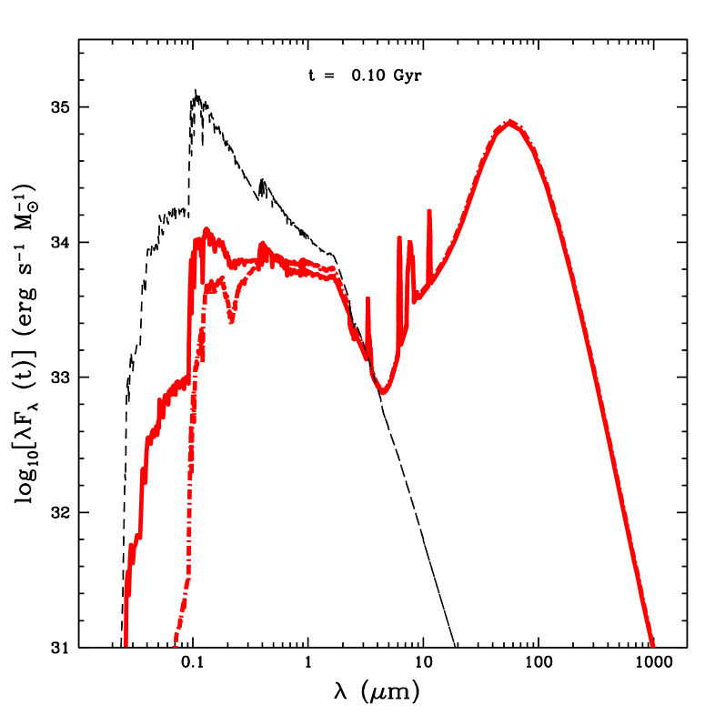
Figure 10: Snapshot of the full wavelength range synthetic spectrum of a typical starburst galaxy with a star formation time scale of 0.1 Gyr and $f_{\rm H}=1$ taken at time $t=10$ Gyr and corresponding to $\tau_{V}^{\mathrm{z}}\simeq 1$ (see bottom left panel of Fig. 6). The initial gas mass available for star formation has been renormalized to $M_{g}(0)=M_{tot}=1\leavevmode\nobreak\ M_{\odot}$ (see eq 2), the real initial value being $M_{g}(0)=10^{12}\leavevmode\nobreak\ M_{\odot}$. The line coding is the same as in Fig. 9.

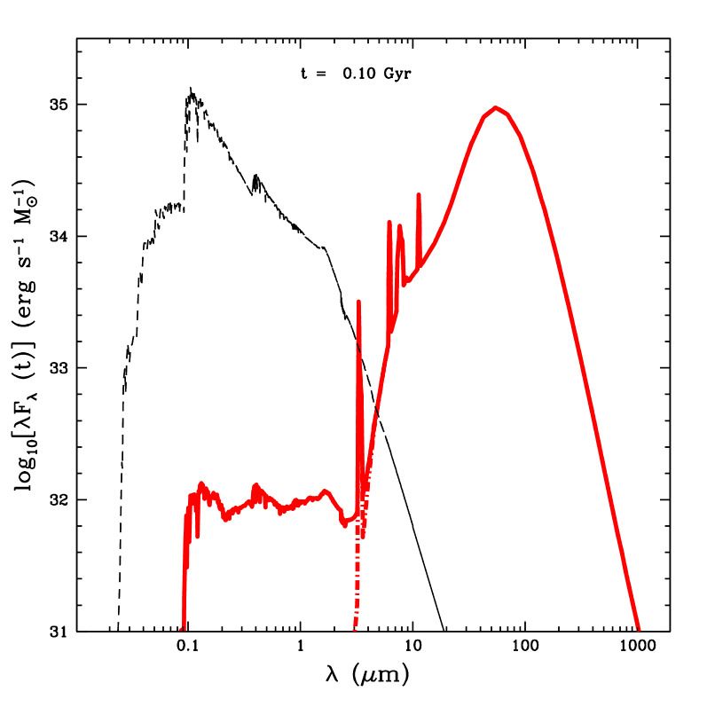
Figure 11: Same spectrum as in Fig. 10 but for $f_{\mathrm{H}}=100$ thus corresponding to $\tau_{V}^{\mathrm{z}}\simeq 100$. The real initial gas mass available for star formation is still $M_{g}(0)=M_{tot}=10^{12}\leavevmode\nobreak\ M_{\odot}$ (see eq 2). For the screen geometry (dot–dashed line), the level of the flux below 2 $\mu$m is negligible.

The important thing to notice is that for normal spirals, the amount of luminosity absorbed by dust is about half the luminosity produced by star formation, whereas for a starburst where the optical depth is calculated with the same prescription, the luminosity released in the IR is already twice as large as the luminosity emitted in the optical. This is mainly due to the fact that, in starbursts, star formation takes place on a time scale which is much shorter than in normal spirals, so that the stellar population has less time to grow old and it emits most of its flux in the UV/optical window where absorption is higher. The other important point to notice is that, when the objects remain marginally optically thin (with $\tau_{\lambda}^{\mathrm{z}}\mathrel{\hbox{\hbox to0.0pt{\hbox{\lower 4.0pt\hbox{$\sim$}}\hss}\hbox{$<$}}}1$), which is the case for the objects plotted in Fig. 9 and 10, the UV/near–IR SEDs (except maybe at wavelengths $<2000$ Å) are fairly robust as they do not depend sensitively on the geometry of the distribution of stars and dust.

For compact starbursts, the optical depth can increase by about two dex (we model these objects by putting our concentration factor $f_{\mathrm{H}}=100$), and, as shown in Fig. 11, two important things happen. First of all, the ratio of the far–IR to optical fluxes is multiplied by a hundred, which was to be expected. Second, and less trivial is that, depending on the geometry adopted, the shape of the optical spectrum can undergo drastic changes. For instance, if one compares figures 10 and 11, it is obvious that, for an oblate ellipsoid geometry, the shape of the stellar spectrum is quite independent of the value of the concentration parameter $f_{\mathrm{H}}$, and the optical SED just undergoes an attenuation of a couple of dex. On the contrary, for an extreme geometry like the screen model, the change is so drastic that the stellar spectrum that was present with $f_{\mathrm{H}}=1$, has totally disappeared for $f_{\mathrm{H}}=100$. Of course, this is purely a test case, for which the radiative transfer can be solved analytically, and the absorption (neglecting inclination) varies exponentially with the optical depth, but nevertheless, it is very illustrative of the sensitivity of the optical spectrum to the dust distribution relative to stars. The explanation of this dependency is that in the case of the oblate ellipsoid geometry, we have a homogeneous mix of dust and stars, so when the optical depth increases we still see the light coming from the stars contained in the “outer peel” of the galaxy. On the contrary, for the screen geometry, the wall of dust in front of the stars just thickens, and does not let any light go through at all.

Figure 12: Time evolution of the luminosities and colors of a galaxy with different star formation time scales and $f_{\rm H}=1$. Coding for the lines is the same as in Fig. 6, top left panel. The initial gas mass available for star formation is $M_{g}(0)=M_{tot}=10^{12}\leavevmode\nobreak\ M_{\odot}$ renormalized to $1\leavevmode\nobreak\ M_{\odot}$, and $L_{\odot}$ stands for solar bolometric luminosity.

Another point we would like to emphasize is the robustness of the dust emission spectrum. As a matter of fact, the level of flux for all wavelengths $>10\mu$m differs by less than 20% between “compact” starbursts (Fig. 10) and “normal” starbursts (Fig. 11) even if the absorption of the starlight is two dex higher for a compact starburst. This is due to the fact that the starlight is absorbed in a narrow wavelength range (typically 3 $\mu$m wide) and re–emitted over a much larger wavelength range (typically 1000 $\mu$m wide). Moreover, the extra quantity of starlight absorbed by the compact starburst represents a very small fraction of the bolometric luminosity $L_{\mathrm{bol}}$ of the object (and hence a very small fraction of the total $L_{\mathrm{IR}}\simeq 2/3L_{\mathrm{bol}}$). These combined effects have the dramatic consequence that one cannot predict the visible spectrum of an ULIRG! However, one should be aware that the shape of the IR/submm SED is very likely to be altered in compact starbursts, due to absorption of dust re–processed photons by other dust grains. When the optical depth reaches values as high as $\approx$ 100 in the V band, one can expect it to still be of the order of 10 at 3 $\mu$m, and more or less of the same value up to 30 $\mu$m because of the silicate absorption features around 10 and 25 $\mu$m (see Fig. 6). Our simple model does not account for such self–absorption explicitly, although one could argue that in principle it is more or less naturally accounted for, simply because of the way we build our spectral library from the phenomenological colors of IRAS galaxies. To sum things up, this effect should result in an important decrease of the strength of PAH features in highly obscured starbursts, which emit more than 90 $\%$ of their luminosity in the far–IR, and for this reason, it should be present in IRAS observations of ULIRGs which we use to build our spectral library. We therefore believe that our conclusion about the overall robustness of the IR SEDs still holds when dust self–absorption is explicitly taken into account.

Figure 13: Same as in Fig. 12 but with $f_{\rm H}=100$.

In Fig. 12 and 13, we quantify these changes a bit further by plotting integrated quantities and broad band colors. As expected, before 3 Myr, there is no IR flux, because no stars have yet exploded. So the ISM is not enriched with metals yet, and there is no dust. After 3 Myr, the metallicity starts growing, along with the dust content and the IR luminosity of the galaxy, while in the same time more gas gets turned into stars. As the optical depth is a function of both the metallicity and gas content, the IR luminosity reaches a maximum and then decreases. In fact, things are more complicated because this behavior depends on the stellar emission spectrum. But, as shown in the same plot (Fig. 12), the optical luminosity has a similar evolution, which is the result of a competition between stars forming at a rate which decreases with time because it is proportional to the gas content of the galaxy, and the ageing of these same stars.

What one notices at first glance when one compares Fig.  12 and 13, is that the global behavior is similar to what has previously been mentioned. The shapes of the spectra are very much alike (mainly because the oblate ellipsoid geometry does not alter significantly the features and the extinction curve as previously discussed) in the sense that the colors (especially B-V) are not noticeably different. Otherwise, the variations of the plotted variables are those expected when one boosts extinction: the IR luminosity increases, the optical luminosity drops, and the absolute magnitudes in B and K increase.

The next step after checking the self–consistency of the model consists in testing the spectra against real data in the full wavelength range.

Figure 14: Flux ratio IRX= $\log_{10}$ (FIR/F220W) as a function of UV spectral slope $\beta$. Data is from Meurer et al. (1997) and Kinney et al. (1994). Galaxies with different star formation time scales are overplotted. Coding for the lines on top panel is : solid for $t_{*}=0.1$ Gyr (thin line $f_{\rm H}=1$ and thick line $f_{\rm H}=100$), dotted line for $t_{*}=1.0$ Gyr, and dashes for $t_{*}=10.0$ Gyr (the thickness coding remaining the same). For the bottom panel, isochrones are plotted for different $t_{*}$ ranging from $0.1$ to $10$ Gyr. Coding for times at which isochrones are taken is indicated in the panel. Once again a thin line stands for $f_{\rm H}=1$ and a thick line for $f_{\rm H}=100$. See text for more details and figure 15 to estimate the starting values of $\beta$ and IRX in the bottom panel.

Fig. 14 and 15 show how the models compare to observations in the UV and far–IR simultaneously. The InfraRed eXcess (IRX) — which is just the decimal logarithm of the ratio of the far–IR flux (as estimated from IRAS observations) and the flux measured in the F220W filter of the Hubble Space Telescope (see Meurer et al. Meurer et al. (1995)) —, is shown both as a function of time (Fig. 15) and as a function of the UV spectral slope $\beta$ — which is defined as the power law index of the UV continuum $F_{\lambda}(\lambda)\propto\lambda^{\beta}$ between 1250 Å  and 2600 Å  , (see Calzetti et al. Calzetti et al. (1994) for details) — (Fig. 14).

Figure 15: Time evolution of the flux ratio IRX and UV spectral slope $\beta$ of galaxies with different star formation time scales. Coding for the lines on both panels is as follows: solid line stands for $t_{*}=0.1$ Gyr, dotted line for $t_{*}=1.0$ Gyr and dashes are for $t_{*}=10.0$ Gyr. In the top panel, the thin line represents models without extinction, the thick line, models with $f_{\rm H}=1$ and the very thick line, models with $f_{\rm H}=100$. Obviously, for the bottom panel, there is no thin curve, but the thickness coding remains the same in the other two cases.

There are a few important things to notice on these figures. In particular, (upper panel of Fig. 15), one can see that, for our geometry (oblate ellipsoid), the UV spectral slope remains negative whatever the value of $f_{\rm H}$, and that, in order to get (almost) flat spectra in the UV (i.e. $\beta\simeq 0$) for starbursts, we need to invoke a higher extinction by setting $f_{\rm H}=100$.

It is striking that it is almost impossible to obtain positive values of $\beta$ with reasonable values of the star formation rate and extinction. Of course, this statement depends on the geometry as well as on the IMF, but one would have to come up with a very ad–hoc combination of these two parameters in order to change the sign of $\beta$. Furthermore, as shown on the same figure (bottom panel), higher values of $\beta$ are not correlated with a strong IRX. They are reached before the IRX attains its maximum level. This just means that if one demands that the geometry be the homogeneous oblate ellipsoid and the IMF be Salpeter, one would have to advocate a column density at least a 1000 times larger in starbursts than in normal spirals (the metallicity dependence becomes second order due to the fact that the peak in the time evolution of $\beta$ appears very early) in order for the extinction to be sufficient to change the sign of $\beta$ ($f_{\rm H}=1000$ in this case, and $\beta$ reaches a maximum value of 0.27).

However, as can be read in Fig. 14, the vast majority of galaxies have negative UV continuum slopes, and therefore, the models are able to span the whole data range quite naturally. As a matter of fact, the spectral slope of the extinction–free starburst is $\beta\simeq-2.8$ for $t<0.02$ Gyr , in agreement with what is generically used Steidel et al. (1999). Furthermore, the predicted reddening is $0.04<E(B-V)<0.4$ (mainly depending on $f_{\rm H}$) for $t<$0.1 Gyr, in fair agreement with what is derived in LBGs under the assumption of a universal (averaged over 0.1 Gyr) $\beta\simeq-2.5$ Steidel et al. (1999).

Figure 16: Best fit model (see text for details) for galaxies extracted from a sub-sample of the Virgo Cluster Catalogue (Boselli et al., 1998), and ULIRGs taken from the sample described in Rigopoulou et al. (1996). As mentioned in the text, this is illustrative of the ability of the model to capture the characteristic features of the objects and there is an important degeneracy between the different parameters ($t_{*}$ and $t$) of the fit. Objects are ordered with increasing $L_{\rm IR}$ from top to bottom and from left to right.

5.1 Fitting Observed Galaxies

The next step is to test the ability of our models to describe multi–wavelength flux measurements of a broad class of objects, from normal galaxies that emit approximatively $30$ % of their bolometric luminosity in the IR, to monsters which have $L_{\mathrm{IR}}/L_{\rm B}\simeq 100$.

To achieve this comparison, we simply select from the literature a sample of galaxies for which fluxes in the UV, optical, IR and submm are available. We also pick the sample in order to have galaxies with total IR luminosities (as estimated from IRAS observations, see e.g. Sanders and Mirabel Sanders and Mirabel (1996)). All the galaxies we show here are taken from samples described in Rigopoulou et al. Rigopoulou et al. (1996) for ULIRGs, and Boselli et al. Boselli et al. (1998) for normal spirals. We also add to the list the close–by LIRG M82 for which our multi–wavelength data availability criterion is fulfilled (see Hughes et al. Hughes et al. (1994) and references therein). We sum up the properties of the selected objects in table 1.

Table 1: Properties of the different objects for which individual fits were achieved. Values given for the absolute magnitudes are derived from the best fit spectrum, i.e. the spectrum of the galaxy which age $t$ and characteristic star formation timescale $t_{*}$ minimize the $\xi^{2}$. For $L_{\mathrm{IR}}$, values reported are obtained by integrating the spectra between 3 $\mu$m and 1000 $\mu$m, whereas, for $L_{\mathrm{OPT}}$, we have integrated the spectra between 100 Å  and 3 $\mu$m. SFR and $\tau_{\mathrm{V}}$ are indicative values that are derived from the best fit model.

Object Name	$t_{*}$ (yr)	$t$ (yr)	D (Mpc)	$M_{B}$	$M_{K}$	$L_{\mathrm{IR}}$ ($L_{\odot}$)	$L_{\mathrm{OPT}}$ ($L_{\odot}$)	SFR ($M_{\odot}$ yr-1)	$\tau_{\mathrm{V}}$
VCC 0836	109	6.7 109	17	-14.7	-18.9	1.7 108	3.0 108	1.0 10-2	0.6
VCC 1003	109	1.4 1010	17	-14.2	-18.2	2.1 107	1.8 108	2.3 10-3	0.1
VCC 1043	109	1.4 1010	17	-14.5	-18.5	4.1 107	2.4 108	3.0 10-3	0.1
VCC 1554	1010	3.2 109	17	-16.0	-18.8	6.9 108	5.2 108	1.0 10-1	0.6
VCC 1690	109	9.3 109	17	-14.8	-18.8	7.8 107	3.1 108	5.8 10-3	0.3
VCC 1727	109	1.1 1010	17	-14.5	-18.6	5.0 107	2.5 108	3.8 10-3	0.2
VCC 1972	1010	3.4 109	17	-15.4	-18.4	3.1 108	3.2 108	6.0 10-2	0.6
VCC 1987	1010	3.3 109	17	-15.3	-18.2	2.7 108	2.9 108	5.4 10-2	0.6
M 82	5 108	9.0 107	4.2	-19.3	-22.9	6.0 1010	1.6 1010	9.1 100	2.2
Arp 220	108	5.0 107	108	-19.4	-23.7	1.6 1012	2.2 1010	2.7 102	75
Mrk 273	108	3.0 107	222	-20.7	-25.0	2.6 1012	7.1 1010	4.2 102	34
UGC 05101	108	2.0 107	240	-20.9	-25.3	1.7 1012	9.3 1010	3.0 102	15
IRAS 05189-2524	108	3.0 107	256	-21.3	-26.1	2.7 1012	1.6 1011	4.6 102	34
IRAS 08572+3915	108	2.0 107	349	-20.7	-23.8	2.4 1012	4.7 1010	4.5 102	15
IRAS 12112+0305	108	5.0 107	435	-20.4	-24.6	3.4 1012	5.1 1010	6.6 102	56
IRAS 14348-1447	108	3.0 107	495	-20.9	-25.0	4.0 1012	7.8 1010	6.5 102	34
IRAS 15250+3609	108	3.0 107	319	-20.2	-24.4	2.0 1012	4.3 1010	3.3 102	34

The parameters that we consider free when we perform the fit are the star formation characteristic time–scale $t_{*}$, and the age of the galaxy $t$. The fits are obtained by a standard $\chi^{2}$ minimization procedure, although we are aware that it has not much statistical significance, mainly because the number of data points used to perform the fit is too small (at most 17 fluxes at different wavelengths). Moreover, the assumption that errors are distributed normally in the statistical sense (which is a requirement for a real $\chi^{2}$ procedure to be valid) probably does not hold. Typical values of the parameters $t$ and $t_{*}$ for the objects represented in the different panels of Fig. 16 can be read in table 1, along with typical properties derived from the best fit model. For the remaining objects of table 1, spectra are available from the authors upon request.

The results of the method we use to obtain the fit can be summarized in the following way, depending on the nature of the fitted objects:

• In the case of the ULIRG sample (in which we include M82 which is not an ULIRG), we find that for most objects, an old population (with a typical age of 10 Gyrs) with the same extinction as the starburst population ($f_{\rm H}=100$) is required to account for the excess of flux in the near–IR (around 1-2 $\mu$m). This is due to the fact that even in our simple modelling, we cannot assume that the measured flux is entirely due to the burst, and we have to take into account the previous star formation history of the galaxy. Clearly, in some cases, there is a degeneracy between $t_{*}$ and this population. This can be understood if one keeps in mind that increasing $t_{*}$ simply means that the stellar population builds up more slowly, and consequently has time to grow old and therefore emits more flux in the near–IR.
  

• For the sample of normal spirals, we allow the same parameters $t_{*}$ and $t$ to vary, but we take $f_{\rm H}=1$. We then add in a few cases a heavily extinguished starburst ($f_{\rm H}=100$) to account for the missing far–IR flux. Once again, this is due to the fact that having just one characteristic time scale for star formation in our model implicitly assumes that, for these objects, all the measured flux comes from the quiescent continuous star formation history of the galaxy, which might describe the average properties of a sample of galaxies, but is too crude when one deals with individual objects in an IR–selected sample.

From all the individual objects fitted, we were then able to extract a sequence of galaxies with different total IR luminosities. This is shown in Fig. 17 (in the spirit of Sanders & Mirabel Sanders and Mirabel (1996)) .

Figure 17: Sequence of galaxies taken from our best fit models (see table 1) with different total IR luminosities as in Sanders and Mirabel 1996. Distances to spiral galaxies in the Virgo Cluster are taken to be 17 Mpc. For the ULIRGs, distances are estimated by Sanders et al. (1988), rescaled to $H_{o}=$ 50 km s^-1 Mpc^-1. Coding for the lines gives the name of each object: thin solid line: VCC 1003; thin short–dashed line: VCC 1727; thin dotted line: VCC 1554; thin long–dashed line: VCC 1987; thick dot–dashed line: M82; thick short–dashed line: Arp 220; thick dotted line: IRAS 15250+3609; and thick solid line: IRAS 12112+0305.

One can see in this figure that, as the IR luminosity increases, the near–IR to UV spectral slope becomes shallower, and the characteristic features like the 4000 Å  break are smeared out. This is the result of a combination of lower absorption and older stellar population for the sample of normal spirals as opposed to higher extinction and younger stellar population for the ULIRGs. However, the figure is somewhat misleading, because one could also see a luminosity sequence in the UV/near–IR SEDs that correlates with $L_{\mathrm{IR}}$. As pointed out earlier in the text, there is no such sequence, for the simple reason that the UV/near–IR SED is extremely sensitive to the relative distribution of stars and dust in heavily obscured objects. For instance, Arp 220 has a SED in this wavelength range similar to M82 and its $L_{\mathrm{IR}}$ is about 100 times larger (see table 1). Finally, the peak of the infrared emission gets shifted towards higher temperatures or equivalently towards shorter wavelengths as the total IR luminosity of the object increases.

6 A Guide to High–z Galaxies

The model described in the previous sections is designed to match available multi–wavelength data of local galaxies. In this section, we use the template spectra derived from the model to make predictions for objects which look like these local galaxies.

Figure 18: Observer– frame spectrum of best fit model of the ULIRG galaxy IRAS 14348-1447 at increasing redshifts, for a cosmology where $H_{o}=$ 50 km s^-1 Mpc^-1, $\Omega_{o}=1$ and $\Omega_{\Lambda}=0$.

More specifically, we show in Fig. 18 how the brightest ULIRG from our sample would look at different redshifts. We would like to draw the attention of the reader to the crucial effect of the so–called negative k–correction at submm wavelengths which makes such objects as luminous at $z\simeq 5$ as at $z\simeq 0.5$ for wavelengths ranging between 400 and 900 $\mu$m.

Figure 19: Apparent magnitude for 3 objects, the “normal” spiral VCC 836 of the Virgo Cluster (solid line), the close–by LIRG M82 (dotted line), and the ULIRG IRAS 14348-1447 (dashed line), as a function of redshift, for an Einstein–de Sitter cosmology where $H_{o}=$ 50 km s^-1 Mpc^-1, $\Omega_{o}=1$ and $\Omega_{\Lambda}=0$. Symbols are galaxies from table 1. Dot–dashed line is a model spiral with $t_{*}=3$ Gyr and an initial gas mass available for star formation of $M_{g}=10^{10}\leavevmode\nobreak\ M\odot$ that formed at redshift 5, and for which the evolution correction is included.

In Fig. 19 and 20, we show optical/near–IR properties that various classes of local objects (from small normal spirals to bright ULIRGs) would have, if they were located at high redshift. The two different pictures represent two different cosmologies (Standard CDM and $\Lambda$CDM, see figure captions for details), and the differences induced by this are of the order of 0.5 magnitudes in the various filters. Also the dot–dashed line shows the evolution effects one expects to measure on the spectrum of a spiral galaxy which forms at redshift 5 with an initial gas mass $M_{g}(0)=10^{10}\,M_{\odot}$.

Figure 20: Same as Fig. 19 for a flat cosmology where $H_{o}=$ 65 km s^-1 Mpc^-1, $\Omega_{o}=0.3$ and $\Omega_{\Lambda}=0.7$.

Fig. 21 and 22 are far–IR/submm properties of the same classes of objects. Here again, the important thing to notice is that the change in fluxes due to the different cosmologies is quite small (less than 30 %) at any wavelength.

Figure 21: Apparent flux for the same objects in different IR/submm wavebands, as a function of redshift for the Einstein–de Sitter cosmology. Coding for the lines is the same as in Fig. 19

.

Figure 22: Same than Fig. 21 for the flat cosmology with a non–zero cosmological constant. Coding for the lines is the same as in Fig. 19.

Eventually, Fig. 23 shows the time evolution of UV luminosities $\lambda_{2800}L_{\lambda_{2800}}$, $\lambda_{1600}L_{\lambda_{1600}}$ (left panel) and IR luminosity $L_{\rm IR}$ (right panel), considered as functions of the star formation rate. We remind the reader that the SFR time evolution is driven by equation 4, and that our galaxies are considered as isolated objects (“closed box” approximation). The interesting thing to note is the tightness of the correlation between $L_{\rm IR}$ and SFR over the five orders of magnitudes spanned by the galaxies we picked.

Figure 23: Star formation rate against luminosity at 2800 Å  and 1600 Å  (left panel), and total infrared luminosity (right panel). Symbols represent quantities derived from our best fit models, some of which can be read from table 1. For clarity, both these quantities and curves at 1600 Å  have been arbitrarily shifted up by two decades. Coding for the lines is the following: solid for a galaxy with initial gas mass $M_{g}(0)=10^{8}\,M_{\odot}$, $t_{*}=1$ Gyr and $f_{\mathrm{H}}=1$; dotted line for a galaxy with initial gas mass $M_{g}(0)=10^{10}\,M_{\odot}$, $t_{*}=0.5$ Gyr and $f_{\mathrm{H}}=10$; dashed line for a galaxy with initial gas mass $M_{g}(0)=10^{11}\,M_{\odot}$, $t_{*}=0.1$ Gyr and $f_{\mathrm{H}}=100$. The curves show time evolution for the above mentioned objects for ages ranging from $t=$ 0.01 (maximum star formation rate and luminosities) to 15 Gyr (minimum star formation rate and luminosities). The straight lines represent least square fits with values for parameters given in the text.

One could point out that there seems to be a correlation between the UV luminosities and SFR too, but, looking carefully at Fig. 23, this holds only for SFR smaller than a few $M_{\odot}$ yr^-1. This is obviously due to the high extinction of all the objects that are massively forming stars (SFR $>$ 100 $M_{\odot}$ yr^-1): their UV luminosities are not significantly different from objects with more normal SFRs (up to 10 $M_{\odot}$ yr^-1). However, we emphasize that this should be viewed as a theoretical correlation, because the points plotted on Fig. 23 are deduced from the best fit model. Nevertheless, the mathematical expression we get from simply fitting this “data” with a power law is $L_{\rm IR}\leavevmode\nobreak\ (L_{\odot})\leavevmode\nobreak\ =\leavevmode\nobreak\ 7.7\leavevmode\nobreak\ \times\leavevmode\nobreak\ 10^{9}\leavevmode\nobreak\ ({\rm SFR}\leavevmode\nobreak\ /\leavevmode\nobreak\ M_{\odot}\leavevmode\nobreak\ {\rm yr}^{-1})^{0.95}$ where the exponent of the SFR is remarkably close to 1. The same fitting method for the UV luminosities yields : $\lambda_{2800}\leavevmode\nobreak\ L_{\lambda_{2800}}\leavevmode\nobreak\ (L_{\odot})\leavevmode\nobreak\ =\leavevmode\nobreak\ 2.0\leavevmode\nobreak\ \times\leavevmode\nobreak\ 10^{8}\leavevmode\nobreak\ ({\rm SFR}\leavevmode\nobreak\ /\leavevmode\nobreak\ M_{\odot}\leavevmode\nobreak\ {\rm yr}^{-1})^{0.62}$ and $\lambda_{1600}\leavevmode\nobreak\ L_{\lambda_{1600}}\leavevmode\nobreak\ (L_{\odot})\leavevmode\nobreak\ =\leavevmode\nobreak\ 2.4\leavevmode\nobreak\ \times\leavevmode\nobreak\ 10^{8}\leavevmode\nobreak\ ({\rm SFR}\leavevmode\nobreak\ /\leavevmode\nobreak\ M_{\odot}\leavevmode\nobreak\ {\rm yr}^{-1})^{0.58}$ with exponents fairly different from unity. Furthermore the scatter is definitely more important. All this points out that it is indeed very important to have a fair estimate of the $L_{\rm IR}$ of high–redshift galaxies if one wants to derive realistic values for their SFRs.

7 Conclusions

In this paper, we have described a simple model which enables us to reproduce the far–UV to submm SEDs of observed galaxies, with a possible extension to radio wavelengths. The specificity of our model is the fact that it self–consistently links starlight and light reprocessed by dust to derive the global spectra of galaxies. We hereafter summarize the main assumptions of our work that attempts to be as phenomenological as possible.

To obtain SEDs of synthetic stellar populations, we couple spectrophotometric and chemical evolutions in a simple way, under the assumptions of a constant IMF (we take Salpeter IMF) and no gas inflows/outflows (closed–box). Once stellar SEDs are computed, we use a phenomenological extinction curve that reproduces the observed metal–dependent trend in the SMC ($Z=1/5\,Z_{\odot}$), LMC ($Z=1/3\,Z_{\odot}$) and Milky Way ($Z=\,Z_{\odot}$). The optical thickness can be computed e.g. under the assumption of no gas inflows/outflows. A simple oblate geometry where stars and dust are homogeneously mixed finally gives the obscuration curve. The absorbed luminosity is redistributed at IR/submm wavelengths with a phenomenological model involving various dust components that reproduce the local correlation of IRAS and submm flux ratios with IR luminosity. The stellar and dust SEDs are then coupled. In this simple approach, the predictions depend on the SFR timescale, galaxy age, and size of gas disk that is simply parameterized with the fudge factor $f_{\mathrm{H}}$.

We have shown that the results derived separately for the UV/optical part of the spectrum and the far–IR/submm luminosity distribution are robust in the sense that they are very close to the results obtained independently by other authors. The predicted stellar SEDs are in good overall agreement with other predictions available in the literature, in spite of different origins for the stellar data. The differences are mainly due to the fact that the late stages of stellar evolution (TP–AGB and post–AGB) are not included in our modelling. The dust SEDs are in good agreement with those of Maffei Maffei (1994), who does not use submm data and takes slightly different components for the dust. The differences amount to at most a factor 2, and decrease with increasing luminosity.

Furthermore, we have demonstrated that the results of the observational and theoretical works on extinction by Calzetti et al. Calzetti et al. (1994) and Meurer et al. Meurer et al. (1995) can be naturally interpreted in the framework of our model as geometrical effects in the relative dust/star distributions. Indeed, in the optically–thick regime with optical depth $\tau_{\mathrm{V}}^{z}\simeq 100$, we observe a flattening and smearing of the $\langle A_{\lambda}\rangle_{i}$ curve — as reported by Calzetti et al. Calzetti et al. (1994) — that depends on the way dust and stars are distributed. The obscuration curve is in good agreement with Calzetti’s, though it is less “grey”. A possible explanation is that Calzetti’s starbursts are more metal–rich on average, than our model starbursts that start from zero metallicity. The spectral slope of the extinction–free starburst is $\beta\simeq-2.8$ for $t<0.02$ Gyr , in agrement with what is generically used Steidel et al. (1999). The predicted reddening is $0.04<E(B-V)<0.4$ for $t<$0.1 Gyr, in fair agreement with what is derived in LBGs under the assumption of a universal $\beta\simeq-2.5$ Steidel et al. (1999) for the UV slope of galactic spectra without extinction. The relation of the IRX to $\beta$ reproduces the observed trend, provided $f_{\rm H}=$ 100 for the most extinguished starburts, and points towards an age of $t=$ 0.01 Gyr for the bursts, though part of the scatter can be interpreted as larger ages.

The synthetic SEDs that are produced illustrate the large range of IR/optical luminosity ratios. A striking but obvious result is that the optical spectrum of a LIRG or ULIRG–type galaxy is extremely sensitive to the details of the dust distribution. This makes the predictions on the optical counterparts of high-z dusty objects difficult to assess.

We have gathered a small sample of nearby galaxies that have been extensively observed at several wavelengths in the optical/IR/submm/radio range. The fit of the overall continuum with our SEDs provides us with a way of interpolating between the data points under assumptions that have a physical meaning. We then generate a sequence of galaxies with IR luminosities that span several orders of magnitude. The spectral trend is very similar to what has been shown by e.g. Sanders & Mirabel Sanders and Mirabel (1996) on a smaller sample. We have established that there is a very good correlation between the star formation rate and the bolometric infrared luminosity, and we have calibrated the relation. In contrast, the UV fluxes in these objects are strongly affected by extinction. Template spectra of the 17 objects listed in table 1 generated with STARDUST, are available upon e–mail request ( devriend@iap.fr or guider@iap.fr ) and can be used for studies of local and distant samples.

We defer the study of high–z sources to forthcoming papers. These SEDs have been explicitly designed to be implemented into SAMs of galaxy formation and evolution where the basic free parameters ($t_{*}$, $t$, and the gas column densities) can be computed from general assumptions of the physical processes ruling galaxy formation. The remaining uncertainties are due to the possibility that dust properties at high z can scale differently with metallicity, that perhaps the IMF is not constant, and that gas inflows/outflows can strongly affect galaxy evolution. In a companion paper Devriendt and Guiderdoni (1999), we will implement all this in a simple but explicit cosmological framework to try to derive global properties of galaxies and trace their evolution. But the final goal is to work with more realistic codes of galaxy formation and evolution, especially those which take into account the merging histories of dark matter halos (e.g. Kauffmann et al. Kauffmann et al. (1993), Baugh et al. Baugh et al. (1996), Somerville and Primack Somerville and Primack (1999), Ninin et al. Ninin et al. (1999)).