Mass estimation in the outer regions of galaxy clusters

Abstract

We present a technique for estimating the mass in the outskirts of galaxy clusters where the usual assumption of dynamical equilibrium is not valid. The method assumes that clusters form through hierarchical clustering and requires only galaxy redshifts and positions on the sky. We apply the method to dissipationless cosmological $N$-body simulations where galaxies form and evolve according to semi-analytic modelling. The method recovers the actual cluster mass profile within a factor of two to several megaparsecs from the cluster centre. This error originates from projection effects, sparse sampling, and contamination by foreground and background galaxies. In the absence of velocity biases, this method can provide an estimate of the mass-to-light ratio on scales $\sim 1-10h^{-1}$ Mpc where this quantity is still poorly known.

1 INTRODUCTION

At scales $\la 1h^{-1}$ Mpc, dynamics of galaxy groups and of the central region of clusters give mass-to-light ratios $M/L\sim 20-30\%$ of that required to close the Universe (e.g. ?; ?). Observations of light curves of Type Ia supernovae at redshifts $z<1$ confirm that there might not be indeed enough mass to close the Universe (?; ?; ?). On the other hand, from the analysis of velocity fields on mildly non-linear scales ($\ga 10h^{-1}$ Mpc), we can measure the quantity $\beta=\Omega_{0}^{0.6}/b$ (e.g. ?) where $\Omega_{0}$ is the mean mass density of the Universe and $b$, assumed independent of scale, is the bias parameter, the ratio between the galaxy and the mass overdensity fields. Recent estimates yield $\beta\sim 0.5-1.1$ (e.g. ?; ?). If galaxies cluster more than mass ($b>1$), this result implies large values of $\Omega_{0}$.

At intermediate scales, $\sim 1-10h^{-1}$ Mpc, estimating the mass-to-light ratio is particularly difficult. These scales correspond to the immediate surroundings of rich clusters, the largest non-linear systems forming at the present epoch. Matter is falling onto the cluster for the first time. Therefore, neither dynamical equilibrium nor linear theory are valid descriptions of the dynamics of this falling matter: at these scales, clusters are already in the non-linear regime although not yet virialized.

We can derive constraints on $\Omega_{0}$ from the dynamics of these infall regions on a statistical basis, by modelling the galaxy-cluster cross correlation function (e.g. ?). On a single cluster basis, however, using the spherical infall model to extract information on $\Omega_{0}$ (?) seems impractical, because in hierarchical clustering scenarios random motions are an important component of the velocity field (van Haarlem & van de Weygaert 1993). Nonetheless, the galaxy distribution in redshift space still contains information about the cluster mass (?, DG hereafter).

DG suggest a method for measuring the mass profile at radii larger than the virial radius of galaxy clusters. DG show that, if the redshift space coordinates of the dark matter particles were measurable, we could estimate the mass profile with a $\sim 30\%$ accuracy, independently of the mass and the dynamical state of the halo.

Here, we present an operational method for extracting the mass profile from the redshift space distribution of galaxies within real clusters. This mass estimator relies on kinematic data alone. Thus, the mass estimate is independent of the relative distribution of mass and light, unless galaxies are not good tracers of the velocity field in the infall region. Detailed modelling suggests that velocity bias is very weak on these scales (?; ?). We apply the method to catalogues of galaxies formed and evolved using semi-analytic procedures within the dark matter halos of dissipationless $N$-body simulations. We show that it is indeed possible to measure the mass of clusters to large radii. Because a few hundred galaxy redshifts are required to give reliable results, this measurement is feasible only on rather massive clusters. This method enables us to estimate the value of the mass-to-light ratio on scales $\sim 1-10h^{-1}$ Mpc.

Sections 2 and 3 review the DG interpretation of the galaxy density distribution in the redshift diagram of clusters and the assumptions of their mass estimation method. Section 4 outlines the operational method of extracting the mass profile from the redshift diagram, and Section 6 shows some applications to galaxy clusters extracted from two cosmological models (Section 5). In Appendix A we also describe a method of locating the centre of a galaxy cluster from a list of galaxies with redshift space coordinates.

2 INTERPRETING THE REDSHIFT DIAGRAM

Observations provide three out of the six phase space coordinates of a galaxy. Define the redshift diagram as the plane $(r,v)$, where $r$ is the galaxy angular separation from the cluster centre and $v$ is its line-of-sight velocity relative to the cluster centre of mass.

The spherical infall model predicts the existence of two curves in this plane where the galaxy number density is infinite (?). These caustics define a characteristic “trumpet” shape and enclose galaxies which are, in real space, at distances both smaller and larger than the turnaround radius from the cluster centre. Galaxies outside the caustics are only at distances larger than the turnaround radius. We define the amplitude ${\cal A}(r)$ of these caustics in redshift space as half the difference between the upper and the lower caustic. The sphericall infall model predicts a dependence of ${\cal A}(r)$ on the cosmological density parameter $\Omega_{0}$ (?; DG).

A clean contrast between the regions interior and exterior to the caustics seem indeed evident in the redshift diagrams of some real clusters (?; ?; Geller, Diaferio & Kurtz 1999a; ?). However, it is a challenge to identify the location of the caustics reliably (e.g. ?; ?). ? were the first to use $N$-body simulations of dark matter halos formed in hierarchical clustering scenarios to show that (1) even in redshift diagrams of dark matter particles the caustics can be poorly determined, and (2) the amplitude of the plausible caustics is usually larger than the amplitude predicted by the spherical infall model for a given cosmology. They concluded correctly that the identification of caustics in cluster redshift diagrams is not a reliable method of estimating $\Omega_{0}$.

? did not clarify, however, what ultimately produces the caustics in the redshift diagram of real clusters. DG suggest a heuristic argument to explain both the presence and the amplitude of the caustics. In hierarchical clustering scenarios non-radial motions and substructure obscure the pure radial motion predicted by the spherical infall model and inflate the predicted amplitude of the caustics. How much do random motions inflate this amplitude? In the infall region of a cluster, a galaxy with a large enough velocity can escape the cluster gravitational field in a time shorter than the age of the Universe. We may therefore expect only a few escaping galaxies lying outside the caustic region in the redshift diagram; this fact rapidly decreases the galaxy number density outside the caustics. Thus, the appearence of the “caustics” is related to the local escape velocity rather than to the cosmological density parameter. In other words, the caustic amplitude is a measure of the cluster gravitational potential at a particular distance from the cluster centre.

Of course, we do not have a correlation between caustic amplitude and cluster gravitational potential when a galaxy system falling onto the central cluster has a mass comparable to that of the cluster; in this case, the amplitude of the caustics is related to the gravitational potential of this falling system rather than the cluster itself.

In order to relate the caustic amplitude ${\cal A}(r)$ to the cluster gravitational potential $\phi(r)$ we proceed as follows (DG). Regardless of the stability of the cluster, at any particular shell of radius $r$ the maximum allowed velocity is the escape velocity $v_{\rm e}^{2}(r)=-2\phi(r)$. The line-of-sight component of this escape velocity sets the location and the amplitude of the caustics in the redshift diagram.

Figure 1: Geometry of the problem. An observer $O$ views the cluster centre $C$ along the line of sight $OC$ and the galaxies $A$ and $B$ along the line of sight $OAB$ at angular separation $\psi$ from the cluster centre. The longitudinal angles of $A$ and $B$ are $\theta+\gamma$ and $\theta$, respectively.

We now compute this expected maximum observable velocity. The line-of-sight component of $v_{\rm e}(r)$ at any given angular separation $r_{\perp}$ from the cluster centre is (see e.g. point $B$ in Fig. 1)

$$v_{\rm e,los}(r|r_{\perp})=v_{{\rm e},\theta}(r){r_{\perp}\over r}-v_{{\rm e},r}(r){(r^{2}-r_{\perp}^{2})^{1/2}\over r},$$ (3)

where the longitudinal angle $\theta$ is the angle between the galaxy position vector ${\bf r}$ centered on the cluster and the line-of-sight to the cluster centre. The equation $\partial v_{\rm e,los}(r|r_{\perp})/\partial r=0$ yields the maximum observable velocity along the line-of-sight at fixed angular separation $r_{\perp}$. The radius $r=r_{M}$, where this maximum occurs, generally differs from $r_{\perp}$ and depends on the velocity profiles $v_{{\rm e},r}(r)$ and $v_{{\rm e},\theta}(r)$, i.e. the gravitational potential $\phi(r)$ and the tidal field determining the non-radial component of the velocity field.

We seek an expression for the expected amplitude ${\cal A}(r_{\perp})$ of the caustics which is independent of the form of the escape velocity profiles. Consider the cluster velocity anisotropy parameter $\beta(r)=1-\langle v_{\theta}^{2}+v_{\phi}^{2}\rangle/2\langle v_{r}^{2}\rangle$, where $v_{\phi}$ is the azimuthal component of a galaxy velocity ${\bf v}$, and the angle brackets indicate an average over the velocities of all the galaxies within the volume $d^{3}{\bf r}$ centered on position ${\bf r}$. If the cluster rotation is negligible, $\langle v_{\theta}^{2}+v_{\phi}^{2}\rangle=2\langle v_{\theta}^{2}\rangle=\langle v^{2}\rangle-\langle v_{r}^{2}\rangle$ and we can write $\langle v_{{\rm e}}^{2}(r_{\perp})\rangle$, the mean of the square of the escape velocity on the shell of radius $r_{\perp}$, by combining its line of sight component $v_{\rm e,los}^{2}(r_{\perp})=v_{{\rm e},\theta}^{2}(r_{\perp})$ (equation 3) and $\beta(r_{\perp})$:

$$\langle v_{{\rm e},\theta}^{2}(r_{\perp})\rangle=\langle v_{\rm e}(r_{\perp})^{2}\rangle{1-\beta(r_{\perp})\over 3-2\beta(r_{\perp})}.$$ (4)

Now, define the quantities

$$g(\beta)\equiv{3-2\beta(r_{\perp})\over 1-\beta(r_{\perp})},\quad\quad\phi_{\beta}(r_{\perp})\equiv{2|\phi(r_{\perp})|\over g(\beta)};$$ (5)

$g(\beta)$ contains the information about the anisotropy of the velocity field governed by the infall and the tidal field; $\phi_{\beta}(r_{\perp})$ combines $g(\beta)$ with the potential $\phi(r_{\perp})$ determined by the mass distribution alone. By assuming $2|\phi(r_{\perp})|\simeq\langle v_{\rm e}^{2}(r_{\perp})\rangle$, we can rewrite equation (4) as

$$\phi_{\beta}(r_{\perp})\simeq\langle v_{{\rm e},\theta}^{2}(r_{\perp})\rangle=\langle v_{{\rm e,los}}^{2}(r_{\perp})\rangle.$$ (6)

When $r_{M}\neq r_{\perp}$, $v_{\rm e,los}^{2}(r=r_{M}|r_{\perp})>v_{\rm e,los}^{2}(r=r_{\perp}|r_{\perp})$. Thus, a priori, the true amplitude $\langle v_{\rm e,los}^{2}(r=r_{M}|r_{\perp})\rangle$ of the caustics is larger than $\phi_{\beta}(r_{\perp})$. Moreover, the measured ${\cal A}(r_{\perp})$ can be larger or smaller than $\langle v_{\rm e,los}^{2}(r=r_{M}|r_{\perp})\rangle$ depending on the presence or absence of escaping galaxies in the redshift diagram. However, comparisons with clusters in $N$-body simulations indicate that $\phi_{\beta}(r_{\perp})$, computed with the full phase space information, agrees, within the uncertainties, with the amplitude ${\cal A}^{2}(r_{\perp})$ computed from the redshift diagram (DG; see also Section 6). We can therefore consider ${\cal A}^{2}(r_{\perp})$ as a measure of $\phi_{\beta}(r_{\perp})$

$$\phi_{\beta}(r_{\perp})\rightarrow{\cal A}^{2}(r_{\perp}).$$ (7)

The equation above represents our physical interpretation of the caustic amplitude ${\cal A}(r_{\perp})$ in the redshift diagram of clusters.

Equation (5) clearly shows that non-radial motion is the fundamental ingredient of this interpretation of the caustic amplitude ${\cal A}(r_{\perp})$. In fact, if orbits were radial, $\beta(r_{\perp})=1$, and equation (5) would predict an uncorrect $\phi_{\beta}(r_{\perp})=0$. On the other hand, random motions dominate the velocity field of the virialized region of the cluster. Thus, this interpretation holds both in the central and in the infall region of the cluster.

In conclusion, in redshift diagrams of real systems, we expect a concentration of galaxies around the cluster redshift at any fixed angular separation. Because of infall, we expect a somewhat clear separation between falling galaxies and unrelated galaxies which are more distant than the turnaround radius. Because of random motions, this separation is not as sharp as predicted by the spherical infall model, but it is still apparent, and it is indeed observed (?). Finally, the cluster gravitational potential determines the amplitude of the caustics.

3 ESTIMATING THE INTERIOR MASS

Suppose we have a method to measure ${\cal A}(r)$ and $g(\beta)$. By assuming ${\cal A}^{2}(r)=\phi_{\beta}(r)$, equation (5) readily yields, for the cumulative cluster mass $GM(<r)=r^{2}d\phi/dr$,

$$GM(<r)=-{r\over 2}{\cal A}^{2}(r)g(\beta)\left({d\ln{\cal A}^{2}\over d\ln r}+{d\ln g\over d\ln r}\right).$$ (8)

The two logarithmic derivatives in equation (8) are comparable. Recently, ?  $\!(\!\!$?) has shown that $\beta(r)$ could actually be measured by detecting $N\ga 50$ galaxy wakes in the X-ray emission of clusters. Bent lobes of radio galaxies might also be used to cross-check these measurements; these galaxies will not be useful for actual measurements, however, because the expected number of these galaxies is not larger than $\sim 5$ per cluster (?). In any case, even if we had a measure of $\beta(r)$, a serious problem occurs independently of the method we use to estimate ${\cal A}^{2}(r)$: sparse sampling and background and foreground galaxies will yield a very noisy ${\cal A}^{2}(r)$; therefore its differentiation is not practical even after substantial smoothing (DG).

Nevertheless, a measure of ${\cal A}(r)$ alone can still be used to estimate the cluster mass. DG suggest casting the relation between ${\cal A}(r)$ and $M(<r)$ in the form

$$GM(<r)-GM(<r_{0})=\int_{r_{0}}^{r}{\cal A}^{2}(x){\cal F}_{\beta}(x)dx$$ (9)

where

$${\cal F}_{\beta}(r) = -2\pi G{\rho(r)r^{2}\over\phi(r)}{3-2\beta(r)\over 1-\beta(r)}$$ (10)

$$\equiv {\cal F}(r)g(\beta),$$ (11)

$\rho(r)$ is the cluster mass density profile and

$$\phi(r)=-{GM(<r)\over r}-4\pi G\int_{r}^{\infty}\rho(x)xdx$$ (12)

is the gravitational potential generated by the cluster.

Equation (9) integrates the estimated ${\cal A}^{2}(r)$ rather than differentiating it, thus averaging out its un-physical rapid variations. However, the crucial property of equation (9) is that the function ${\cal F}_{\beta}(r)$ is slowly varying at large radii in hierarchical clustering scenarios, as we will show below. This property is of major importance, because we may assume ${\cal F}_{\beta}(r)={\rm const}\equiv{\cal F}_{\beta}$. Equation (9) then becomes

$$GM(<r)-GM(<r_{0})={\cal F}_{\beta}\int_{r_{0}}^{r}{\cal A}^{2}(x)dx.$$ (13)

Thus, we make the mass estimation method independent of any scale length, implicitly assumed in the function ${\cal F}_{\beta}(r)$, although still dependent on the unknown ${\cal F}_{\beta}$. Of the three equations (8), (9) and (13), only equation (13) turns out to be of practical relevance. We emphasize that equation (13) is justified only in hierarchical clustering scenarios.

Note that the similarity between equation (9) and equation (13) might suggest using an iterative procedure: equation (13) provides the first mass profile from which we can estimate ${\cal F}_{\beta}(r)$ and we can then use equation (9) until convergence is achieved. Unfortunately, ${\cal F}_{\beta}(r)$ contains information on both the mass distribution and the velocity field (equation 11), whereas equations (9) and (13) return information on the mass profile alone. Therefore, we should still make an assumption about $g(\beta)$. However, even in this case, the improvement in the mass estimate is likely to be insufficient to reduce the uncertainty which is introduced by projection effects. These effects actually dominate the problem, as we will show in Section 6.

To justify ${\cal F}_{\beta}(r)={\cal F}(r)g(\beta)={\rm const}$ in hierarchical clustering cosmogonies, first consider the function ${\cal F}(r)=-2\pi G\rho(r)r^{2}/\phi(r)$, and a density profile approximated piecewise by power laws $\rho(r)\propto r^{-\alpha(r)}$. Provided the mass is finite at $r=0$ ($\alpha(r)<3$, when $r\to 0$), and $\phi(r)$ converges at large radii ($\alpha(r)>2$, when $r\to\infty$), we obtain ${\cal F}(r)\propto r^{2-\alpha(r)}/[M(<r)r^{-1}+r^{2-\alpha(r)}]$. At large radii, ${\cal F}(r)$ behaves differently depending on the behavior of $M(<r)\propto r^{3-\alpha(r)}$. If the mass is finite ($\alpha(r)>3$, when $r\to\infty$), ${\cal F}(r)$ decreases as a power law, ${\cal F}(r)\propto r^{-|\alpha(r)-3|}$. If the mass diverges ($2<\alpha(r)<3$, $r\to\infty$), ${\cal F}(r)\sim{\rm const}$. This is the case of interest here.

Figure 2: Filling function ${\cal F}_{\rm NFW}(r)$ for the NFW density profile (equation 14). The bold line is ${\cal F}_{\rm NFW}(r/r_{s})$. Thin lines are ${\cal F}_{\rm NFW}(r)$ for different values of the concentration parameter $c=r_{200}/r_{s}$.

$N$-body simulations of hierarchical clustering scenarios suggest a universal density profile for dark matter halos (?, NFW hereafter). This profile yields a diverging mass and a convergent gravitational potential at the same time, as required by the argument above. However, in this case, $\alpha(r)=3$ when $r\to\infty$, implying $M(<r)\propto\ln(r)$ and

$${\cal F}_{\rm NFW}(r)={1\over 2}{(r/r_{s})^{2}\over(1+r/r_{s})^{2}}{1\over\ln(1+r/r_{s})}$$ (14)

where $r_{s}$ is a scale length defined in terms of the halo concentration $c=r_{200}/r_{s}$, and $r_{200}$ is the radius of the sphere whose average mass density is 200 times the critical density. ${\cal F}_{\rm NFW}(r)$ is not constant in hierarchical clustering scenarios (see Figure 2). However, ${\cal F}_{\rm NFW}(r)$ decreases by $\sim 20$% at most in the radius range $r\in[1,10]r_{200}$ for $c\in[1,7]$. This range of concentration $c$ is typical for massive halos in Cold Dark Matter (CDM) models; in fact, in our $N$-body models (Section 5), 90% of halos more massive than $10^{14}h^{-1}M_{\odot}$ have $c$ in the range $[1.6,5.2]$ with median $c=3.7$.

To see that ${\cal F}_{\beta}(r)={\cal F}(r)g(\beta)$ is also a slowly varying function of $r$, we compute the functions $\beta(r)$ and $g(\beta)$ for massive clusters in our $N$-body simulations (Section 5). Because these two functions do not show strong variations with $r$, the assumption of a slowly varying ${\cal F}_{\beta}(r)$ appears reasonable. We will specify the value of the constant ${\cal F}_{\beta}$ in Section 6.

Finally, it is important to note that the identification of the amplitude ${\cal A}(r)$ of the caustics with the gravitational potential $[\phi_{\beta}(r)]^{1/2}$ at any radius $r$ is independent of the density profile and the dynamical state of the system, provided that random motions contribute significantly to the velocity field and the spherical assumption is a good approximation. On the other hand, the measurement of ${\cal A}(r)$ yields the mass profile $M(<r)$ (equation 13) only when the density profile is proportional to $r^{-\alpha(r)}$, with $2<\alpha(r)\leq 3$ when $r\to\infty$.

4 MEASURING ${\cal A}(r)$

We now outline an operational method for locating the caustics in the redshift diagram of real clusters. Compiling a redshift diagram requires knowledge of the cluster centre and its radial velocity. Appendix A describes how to determine the cluster centre when only the celestial coordinates of the galaxies and their redshifts are available.

In order to determine the amplitude ${\cal A}(r)$ of the caustics at fixed $r$, consider the two-dimensional density distribution function $f_{q}(r,v)drdv$, namely the number of galaxies with projected separation in the interval $(r,r+dr)$ and line-of-sight velocity in the interval $(v,v+dv)$. In the spherical infall model, at fixed $r$, $f_{q}(r,v)$ reaches infinity at the two caustic locations. Random motions, however, wash these two spikes out and $f_{q}(r,v)$ has a maximum close to the cluster redshift; in the absence of massive substructure and foreground and background galaxies, and in the absence of escaping galaxies, the solutions of the equation $f_{q}(r,v)=0$ would determine the amplitude ${\cal A}(r)$. However, this situation never occurs because, even for isolated systems, escaping galaxies can always be present. Thus, $f_{q}(r,v)$ always becomes zero outside the actual location of the caustics.

We therefore need a recipe for choosing a threshold $\kappa$ such that the equation $f_{q}(r,v)=\kappa$ determines the amplitude ${\cal A}(r)$. Moreover, we have to face the non-trivial issue of accurately estimating $f_{q}(r,v)$ where it is close to zero. It is clear that the this task is not easy, because sparse sampling leads to an underestimate of $f_{q}(r,v)$ and the presence of foreground and background galaxies leads to an overestimate of $f_{q}(r,v)$ at the caustic location. We describe the determination of $f_{q}(r,v)$ in Section 4.1. In Section 4.2 we describe the choice of $\kappa$.

4.1 Estimating the redshift diagram density distribution

Consider $N$ galaxies with coordinates ${\bf x}=(r,v)$, where $r$ and $v$ are conveniently rescaled (we come to this issue later). We use an adaptive kernel method (?; see also ?; ?) to estimate the density distribution of galaxies within the redshift diagram

$$f_{q}({\bf x})={1\over N}\sum_{i=1}^{N}{1\over h_{i}^{2}}K\left({\bf x}-{\bf x}_{i}\over h_{i}\right)$$ (15)

where

$$K({\bf t})=\cases{4\pi^{-1}(1-t^{2})^{3}&$t<1$\cr 0&otherwise\cr}$$ (16)

and $h_{i}=h_{c}h_{\rm opt}\lambda_{i}$ is a local smoothing length depending on the local density. The optimal smoothing length is

$$h_{\rm opt}={3.12\over N^{1/6}}\left(\sigma_{r}^{2}+\sigma_{v}^{2}\over 2\right)^{1/2}$$ (17)

where $\sigma_{r}$ and $\sigma_{v}$ are the marginal standard deviations of the galaxy coordinates. The local smoothing factor is $\lambda_{i}=[\gamma/f_{1}({\bf x}_{i})]^{1/2}$ where $f_{1}$ is equation (15) where $h_{c}=\lambda_{i}=1$ for any $i$, and $\log\gamma=\sum_{i}\log[f_{1}({\bf x}_{i})]/N$.

The average degree of smoothing is controlled by $h_{c}$. The optimal $h_{c}$ should minimize the integrated square error between the estimator $f_{q}({\bf x})$ and the true (unknown) density $f({\bf x})$, $\epsilon(h_{c})=\int[f_{q}({\bf x})-f({\bf x})]^{2}d^{2}{\bf x}$. However, it is easy to show that minimizing $\epsilon(h_{c})$ is equivalent to minimizing

$$M_{0}(h_{c})=\int f_{q}^{2}({\bf x})d^{2}{\bf x}-{2\over N}\sum_{i=1}^{N}f_{q}^{(-i)}({\bf x}_{i})$$ (18)

where $f_{q}^{(-i)}({\bf x}_{i})$ is the density estimated at ${\bf x}_{i}$ using all the data points except ${\bf x}_{i}$ (?). Therefore, $M_{0}(h_{c})$ can be estimated with the data alone and we do not need to assume any form for the true density $f({\bf x})$.

We now address the question of rescaling $r$ and $v$, such that we can use spherical smoothing windows of size $h_{i}$. The adaptive kernel method is designed to estimate density distributions of random variables. If this were the case, we could apply the whitening transformation, namely we would linearly transform the data to have a unit covariance matrix (?). Unfortunately, ${\bf x}=(r,v)$ is not a random variable and the elements of the covariance matrix depend on the limits imposed a priori on the redshift diagram.

We therefore have to rescale $r$ and $v$ in a sensible way. Let us use the Hubble constant to have $r$ and $v$ in the same units. It is obvious that, for example, $100$ km s^-1 in the $v$ direction shold not have the same weight as $1h^{-1}\ {\rm Mpc}=100$ km s^-1 in the $r$ direction. We thus rescale $r$ and $v$ such that the ratio $h_{v}/h_{r}$ of the smoothing window sizes along $v$ and $r$ respectively takes a chosen value $q$. Galaxy redshifts have typical uncertainties of $50$ km s^-1. Positions of galaxies within nearby clusters have uncertainties of $\approx 0.02h^{-1}$ Mpc. We thus set $q=25$ and keep this value fixed hereafter. Note however that different values of $q$ in the range $[10,50]$ have little effects on the results.

4.2 Choosing the threshold

We determine the amplitude ${\cal A}(r)$ at fixed $r$ by finding the solutions of the equation $f_{q}(r,v)=\kappa$. Specifically, the first upper and lower solutions $v_{\rm u}$ and $v_{\rm d}$, away from the maximum of $f_{q}(r,v)$ closest to $v=0$, determine the amplitude ${\cal A}(r)=\min\{|v_{\rm u}|,|v_{\rm d}|\}$. Note that the prescription ${\cal A}(r)=\min\{|v_{\rm u}|,|v_{\rm d}|\}$ is equivalent to ${\cal A}(r)=(v_{\rm u}-v_{\rm d})/2$ for an isolated spherically symmetric system. However, our prescription is more robust than ${\cal A}(r)=(v_{\rm u}-v_{\rm d})/2$ against interloper contamination and the presence of massive substructure.

It is clear that, although we have determined $f_{q}(r,v)$ uniquely (except for the choice of $q$), there are an infinite number of thresholds $\kappa$ we can use to determine ${\cal A}(r)$. It seems reasonable to assume that, at least in the central region, the cluster has attained virial stability. Therefore, in this region, the equation $\langle v_{\rm esc}^{2}\rangle_{R}=4\langle v^{2}\rangle_{R}$ must hold, where now the angular brackets indicate an average over the whole sphere of radius $R$, and velocities are three-dimensional. In the data we only have one-dimensional information, and we thus further assume that, if the velocity field is roughly isotropic in the central region, our expression also holds when $v$ is the galaxy line-of-sight velocity and $\langle v_{\rm esc}^{2}\rangle_{\kappa,R}=\int_{0}^{R}{\cal A}^{2}(r)\varphi(r)dr/\int_{0}^{R}\varphi(r)dr$, where $\varphi(r)=\int f_{q}(r,v)dv$; $\langle v_{\rm esc}^{2}\rangle_{\kappa,R}$ is the only $\kappa$-dependent quantity. We can choose $\kappa$ by minimizing the function

$$S(\kappa,R)=|\langle v_{\rm esc}^{2}\rangle_{\kappa,R}-4\langle v^{2}\rangle_{R}|^{2}.$$ (19)

In Appendix A we describe a procedure for locating the cluster centre from a list of galaxy positions. This procedure also identifies the cluster members. In the following, we define $R$ as the mean projected distance of the members from the cluster centre, and $\langle v^{2}\rangle_{R}$ the one-dimensional velocity dispersion of the cluster members.

The amplitude ${\cal A}(r)$ is obviously sensitive to the value of $\kappa$. If $f_{q}(r,v)$ has a rather shallow gradient towards the minimum around the real location of the caustics, a slightly incorrect estimate of $\langle v^{2}\rangle_{R}$ can lead to particularly inaccurate estimates of ${\cal A}(r)$. Thus, in these cases, minimizing $S(\kappa,R)$ will only give a starting value for the choice of $\kappa$. The final value of $\kappa$ can be chosen by hand and the location of the caustics will unfortunately be subjective. This freedom is unsatisfactory. On the other hand, $\kappa$ remains a useful one-parameter tool which quantifies the complexity of the infall region of individual clusters and the contamination of their redshift diagrams by background and foreground galaxies. In any case, this subjective tuning turns out to be necessary in a few cases only, and mainly for one of the two cosmological models we investigate here, which yields the poorest fit to observation. This result suggests that the minimization of $S(\kappa,R)$ is likely to be a robust procedure for real clusters, as the Coma cluster has indeed already shown (?).

To control the contamination by background and foreground galaxies efficiently, we need a final step. Consider the logarithmic derivative $2d\ln{\cal A}/d\ln r=d\ln\phi_{\beta}/d\ln r$; we have $d\ln\phi_{\beta}/d\ln r=d\ln|\phi|/d\ln r-d\ln g/d\ln r$. For any realistic system $d\ln|\phi|/d\ln r\la 0$. Our $N$-body simulations show that $d\ln g/d\ln r\ga-1/2$. Thus, we can safely claim that $d\ln\phi_{\beta}/d\ln r\la 1/2$ should hold for any $r$. To be conservative, we therefore accept only values of ${\cal A}(r)$ which yield $d\ln{\cal A}/d\ln r<1$; otherwise we impose a new value of ${\cal A}(r)$ which yields $2d\ln{\cal A}/d\ln r=1/2$.

Table 1: GIF Simulations

model	$\Omega_{0}$	$\Omega_{\Lambda}$	$h$	$\sigma_{8}$	$m_{p}$	$L$
$\Lambda$CDM	0.3	0.7	0.7	0.90	1.4	141
$\tau$CDM	1.0	0.0	0.5	0.60	1.0	85

Parameters of the two GIF simulations (?) used in this paper. The Hubble constant $h$, the particle mass $m_{p}$, and the comoving size $L$ of the simulation box are in units of $H_{0}=100$ km s^-1 Mpc^-1, $10^{10}$ $h^{-1}$ $M_{\odot}$, and $h^{-1}$ Mpc, respectively.

Figure 3: Profiles of $\beta(r)$, $g(\beta)$, ${\cal F}(r)$, and ${\cal F}_{\beta}(r)$ for the clusters with $M_{200}\geq 10^{14}h^{-1}M_{\odot}$ in the $\tau$CDM (dashed lines) and $\Lambda$CDM (solid lines) models. Bold lines are the median profiles. Shaded areas show the interquartile range of the profiles.

5 NUMERICAL MODELS

In Section 6 we apply our mass estimation method to dissipationless $N$-body simulations where we form and evolve galaxies within their dark matter halos with phenomenological recipes. Here, we briefly describe our cosmological simulations.

5.1 The GIF simulations

We use two $N$-body simulations from the GIF project (?). These simulations use $256^{3}$ dark matter particles to model the evolution, from redshift $z=50$ to the present, of the dark matter density perturbations of a CDM universe with an initial power spectrum

$$P(k)\propto k\{1+[6.4k/h\Gamma+(3k/h\Gamma)^{3/2}+(1.7k/h\Gamma)^{2}]^{1.13}\}^{-2/1.13}$$ (20)

where $k$ is in units of $h$ Mpc^-1, and $\Gamma=0.21$ is a shape parameter (?). The normalization is fixed by the ratio $\sigma_{8}^{2}$ of the variances of the mass and galaxy fluctuations within randomly placed spheres of radius $8h^{-1}$ Mpc. The GIF models are normalized to give the correct abundance of rich galaxy clusters at the present time. The simulations were run with Hydra (?), the parallel version of the AP³M code (?; ?), kindly provided by the Virgo supercomputing consortium (?). The two models we consider here are a flat model with or without a cosmological constant: $\Omega_{0}=0.3$ and $\Omega_{\Lambda}=0.7$ ($\Lambda$CDM) and $\Omega_{0}=1$ ($\tau$CDM). Table 1 summarizes the parameters of these models.

? combine these $N$-body simulations with semi-analytic modelling to form and evolve galaxies within dark matter halos. They provide a detailed description of this procedure and compare the observable properties of the simulated galaxy catalogues with the real Universe in a series of papers (?; ?; ?). The relevant physical processes for galaxy formation include gas cooling, star formation, supernova feedback, stellar evolution, and merging of galaxies. Previous attempts to compare such dissipationless simulations with the real galaxy distribution were based on some high-peak statistical model for galaxy formation or on ad hoc assumptions about the mass-to-light ratio of dark matter halos (e.g. ?; ?). Alternatively, we could consider a full $N$-body/hydrodynamic simulation. However, the current state-of-the-art for such simulations can model only a small volume of the Universe, otherwise their resolution limit is larger than the size of galaxies and their halos (e.g. ?; ?; ?; ?; ?; ?).

The GIF simulations have a resolution limit of $30h^{-1}$ kpc and are suitable for investigating the reliability of our mass estimation method. We can in fact construct mock redshift diagrams with galaxies, along with their observable properties, rather than with dark matter particles alone. Note that, in these models, galaxy samples show only a weak velocity bias, independently of galaxy luminosities, as expected if gravity is the driving force on scales $\ga 1h^{-1}$ Mpc.

As discussed in ?  $\!(\!\!$?), the free parameters entering the galaxy formation recipe have substantial effects on galaxy properties. Here, for consistency, we consider the “fiducial” models which yield reasonable fits to many but not all the observed properties of galaxies; in particular the model luminosity function is a rather poor fit to observation. For the purpose of this paper, it is worth noting that the $\tau$CDM model has a luminosity density in the $B$-band which is a factor $\sim 2$ larger than in real galaxy samples, whereas the $\Lambda$CDM model has a luminosity density a factor $\sim 2$ smaller. In order to quantify the effect of the luminosity function on the derived properties of the galaxy distribution, ? assign new luminosities to the model galaxies, while preserving their luminosity rank in such a way as to reproduce the luminosity function of the Center for Astrophysics (CfA) redshift survey (?) exactly. We therefore have two distinct sets of simulated galaxy catalogues: (1) the SALF catalogues where galaxies have luminosities derived from the semi-analyitic modelling, and (2) the CfALF catalogues where galaxies have luminosities imposed according to the CfA luminosity function.

5.2 Profiles of dark matter halos

Before testing the mass estimation method, we address the robustness of the assumptions described in Section 3, namely whether ${\cal F}_{\beta}(r)$ is a slowly varying function of $r$ in these CDM models.

We identify dark matter halos using a friends-of-friends group finder which links particles closer than 0.2 times the interparticle separation. We take the position of the most bound particle as the centre of the halo. Here, we consider only dark matter halos with $M_{200}\geq 10^{14}h^{-1}M_{\odot}$, where $M_{200}$ is the mass within $r_{200}$. Less massive halos are less interesting for our purpose, because our mass estimation method, which requires the redshifts of a few hundred galaxies, will be applicable to massive clusters only.

Figure 3 shows the median profiles of the relevant quantities of the halos in both models. Shaded areas indicate the interquartile range of the profiles. The velocity anisotropy parameter $\beta(r)$ increases from $\sim 0.2$ to $\sim 0.5-0.6$ between $r=0.1r_{200}$ and $r\sim 3r_{200}$, as radial motions become predominant. Remarkably, this result agrees with the value $\beta\sim 0.5$ estimated by ? for the emission-line galaxies in the ESO Nearby Abell Cluster Survey. At the turnaround radius $r\approx 4-5r_{200}$, $\langle v_{r}^{2}\rangle$ decreases faster than its non-radial counterparts $\langle v_{\phi}^{2}\rangle$ and $\langle v_{\theta}^{2}\rangle$; thus, $\beta(r)$ drops to negative values. Note that $\beta(r)$ is sensibly smaller than one everywhere, indicating that random motions always contribute significantly to the velocity field, as expected in hierarchical clustering scenarios. The function $g(\beta)$ we introduced in Section 2 behaves as $\beta(r)$. More importantly, $g(\beta)$ varies with $r$ slowly, increasing by 30-50% at most between $r=0.1r_{200}$ and $r\sim 2-3r_{200}$. At radii where the Hubble flow dominates, $\beta(r)\to 1$ and $g(\beta)\to\infty$.

To compute the function ${\cal F}(r)$ introduced in Section 3, we need to compute the gravitational potential $\phi(r)$ generated by the halo. We could compute $\phi(r)$ with equation (12) where we replace the upper limit of integration with a maximum radius. However, because the halo density profiles are well approximated by the NFW formula, it is more efficient to obtain a fit to the density profile and compute $\phi(r)$ analytically. This procedure bypasses the problem of subtracting the background at large radii. Figure 3 shows that ${\cal F}(r)$ is slowly varying, as expected. Note that at radii $r\ga 3-4r_{200}$, the derivative of ${\cal F}(r)$ is positive. In fact, the density profiles do not decrease as $r^{-3}$ as predicted by the NFW profile, but rather decrease as $r^{-\alpha}$, with $\alpha\sim 1-2$, because they must approach the background density. Therefore ${\cal F}(r)\sim-\rho r^{2}/\phi$ increases as $r^{3-\alpha}/\ln r$. Note that the statistical spread in the ${\cal F}(r)$ profiles accounts for different concentration parameters $c$. As expected, ${\cal F}_{\beta}(r)$ has a trend similar to the trend of ${\cal F}(r)$, because $g(\beta)$ does not vary strongly. Variations of $g(\beta)$ only make the statistical spread of ${\cal F}_{\beta}(r)$ larger.

Note that the difference between the $\tau$CDM and the $\Lambda$CDM models for each of the four profiles is mainly due to the different physical location of $r_{200}$ in the clusters of the two models: $r_{200}$ identifies a sphere with an average density, in units of the background density, which is larger in the low density universe than in the high-density one.

In conclusion, ${\cal F}_{\beta}(r)$ is not constant in these models, as assumed in equation (13), but it varies by a factor of two at most within $r\sim 3-4r_{200}$. Despite these variations, equation (13) remains a useful recipe, as we show in the next section.

6 GALAXY CLUSTERS

We now apply our caustic location method and mass estimation procedure to simulated clusters. To construct the redshift diagram, we use the centre of the dark matter halo and include galaxies brighter than $M_{B}=-18.5+5{\rm log}h$. This magnitude limit corresponds to an apparent magnitude of $m_{\rm lim}=15.7$ at the distance of Coma ($R=7000$ km s^-1) and is one magnitude brighter than the limit of completeness of our galaxy catalogues (?).

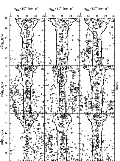
Figure 4: Redshift diagrams of a cluster in the $\Lambda$CDM model viewed along nine different lines of sight. The circles show galaxies brighter than $M_{B}=-18.5+5{\rm log}h$. The bold lines show the identified caustic locations. When the contamination by foreground and/or background galaxies is too heavy for a reliable location of the caustics the method does not proceed further. This situation is represented by merging the caustics into a single horizontal line at the cluster redshift (see right-bottom panel).

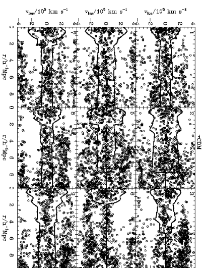
Figure 5: Same as Fig. 4 for a cluster in the $\tau$CDM model.

We also simulate observations of nearby clusters, by randomly choosing the observer’s location on a sphere of radius $R=7000$ km s^-1 centered on the centre of the dark matter halo. We then compile a list of galaxies brighter than $m_{\rm lim}=15.7$ with coordinates $(\alpha,\delta,cz)$ within 10^o from the halo centre; from this list, we locate the cluster centre with the method described in Appendix A. This method usually locates the cluster centre accurately; both this procedure and the one which uses the centre of the dark matter halo directly, yield similar results. Below, we show results where we use the centre of the dark matter halo.

6.1 Caustic Location

Fig. 4 shows the redshift diagrams of a typical cluster in the $\Lambda$CDM model. The nine panels correspond to nine different lines of sight. The galaxies tend to populate a defined region in the redshift diagram. The contrast is quite evident between the galaxies within and outside this region. In most cases, our method seems to locate the caustics, i.e. the borders of this region, correctly.

As discussed in ?, despite the fact that mock redshift surveys extracted from both the $\tau$CDM and the $\Lambda$CDM models do not show structures as sharply defined as in real surveys, the two models still show substantial differences: the $\Lambda$CDM model shows voids and filaments larger than the $\tau$CDM model and yields a better qualitative fit to the real Universe (see ? for a quantitative analysis). These differences also are quite apparent in redshift diagrams of clusters (Figs. 4 and 5), where the density contrast between interlopers and galaxies falling onto the cluster is less evident in the $\tau$CDM than in the $\Lambda$CDM model. Nevertheless, in $\tau$CDM clusters, our method still locates the caustics reasonably well in most cases (Fig. 5).

The different redshift diagrams yielded by the two cosmological models are related to the underlying mass distribution rather than to the galaxy luminosity function. Using the CfALF catalogue decreases the number of galaxies in the redshift diagrams of $\tau$CDM clusters but does not improve the appearence of the caustics. In fact, in this high density universe, clusters are still accreting mass at a large rate at redshift $z=0$. On the other hand, in the $\Lambda$CDM, where using the CfALF catalogue increases the number of galaxies in the redshift diagrams, the accretion rate is substantially smaller and the caustics tend to appear more clearly, as observed in real clusters (?).

In principle, this redshift diagram morphology could be used to distinguish between high and low density universes. For example, we could quantify this difference by using the distribution of the ratio between the number of galaxies lying within the caustics and the total number of galaxies within the redshift diagram. This ratio, of course, depends on the cluster and on the line of sight, but the moments of the distribution should be sensitive to the cosmological model. For example, these ratios for the different lines of sight of the $\Lambda$CDM cluster (Fig. 4) are in the range $[0.32,0.88]$ with median 0.53 (panel 2) and are considerably larger than the corresponding ratios of the $\tau$CDM cluster (Fig. 5): $[0.11,0.55]$ with median 0.39 (panel 7). These distributions appear to be robust against variations of the magnitude limit of the galaxy sample. The feasibility of this kind of statistical tests will be investigated in future work.

In panels 2, 5, and 9 of Fig. 5 the caustics seem to be outside the location we would guess subjectively, because of the heavy contamination by foreground and background galaxies. Our intuition is confirmed by comparing the amplitude ${\cal A}(r)$ of the caustics with the function $[\phi_{\beta}(r)]^{1/2}$ computed from the full six-dimensional phase space information. The upper right panel of Fig. 6 shows all nine estimated profiles for the $\tau$CDM cluster: the ones which tend to overestimate ${\cal A}(r)$ come from the three errant panels. In the other six redshift diagrams and in all the diagrams of the $\Lambda$CDM cluster the agreement is rather good.

Figure 6: Profiles of the two clusters shown in Figs. 4 and 5. The thin lines are the profiles measured from the redshift diagrams. The bold lines in the four upper panels are the true profiles.

It is worthwhile to note, at this point, that our caustic location procedure is essentially an interloper-removal procedure which uses the combined information on the galaxy position and line-of-sight velocity, unlike standard 3-sigma clipping procedures which ignore the position of galaxies (e.g. ?; ?). Our procedure enables us to estimate the mass profile of clusters as a by-product, on the assumption that clusters form through hierarchical clustering.

Let us finally emphasize that our procedure does not remove all the interlopers: in fact, any interloper-removal procedure, which does not separate the galaxy redshift in its Hubble flow and peculiar velocity components, is obviously unable to identify interlopers lying within the caustics in redshift space.

6.2 Mass Profiles

To compute the mass profile from the caustic amplitude, we set ${\cal F}_{\beta}=1/2$ in equation (13), as first suggested by DG, although Fig. 3 shows that the mean value of ${\cal F}_{\beta}$ may be slightly larger; moreover, we set $r_{0}=0$. We thus have

$$GM_{\rm est}(<r)={1\over 2}\int_{0}^{r}{\cal A}^{2}(x)dx.$$ (21)

In writing equation (13) we have assumed that ${\cal F}_{\beta}(r)$ is roughly constant at large $r$. Thus, setting $r_{0}=0$ is justified if ${\cal F}_{\beta}(r)$ is also roughly constant at small $r$ and takes the same values as at a large $r$. In fact, Fig. 3 shows that ${\cal F}_{\beta}(r)\in[0.5,1.0]$ for any $r\la 4r_{200}$, and Fig. 6 shows that the estimate of $M(<r)$ at small $r$ is as good as at large $r$.

The mass profile is recovered within an uncertainty of 50% out to $\sim 8h^{-1}$ Mpc for the $\Lambda$CDM cluster (left middle panel of Fig. 6). For the $\tau$CDM cluster the estimated mass profile is less accurate at those distance, but still within a factor of two.

Finally, the bottom panels of Fig. 6 show the profiles of the $B$-band mass-to-light ratio in units of the mean ratio for the entire simulation box. In the $\Lambda$CDM cluster, the mass-to-light ratio tends to be larger than the universal value at very small radii because of the deficiency of blue galaxies in the central region of clusters in this cosmology (?). At radii $\sim 4-6h^{-1}$ Mpc both models show a mass-to-light ratio consistent with the universal value. Note that for these massive clusters, on average, the mass-to-light ratio within $r_{200}\sim 1.5h^{-1}$ Mpc, computed with the full three-dimensional information, is close to the universal value (see Fig. 15 of ?). This result is consistent with our Fig. 6 where the estimation of the mass-to-light ratio at $r\sim 1.5h^{-1}$ Mpc suffers from projection effects and errors in the mass estimate.

Real clusters, of course, provide a single redshift diagram. The error in the measured value of ${\cal A}(r)$ should depend on the number of galaxies which contribute to the determination of ${\cal A}(r)$. We thus assume that the relative error $\delta{\cal A}(r)/{\cal A}(r)=\kappa/\max\{f_{q}(r,v)\}$, where the maximum value is found along the $v$-axis at fixed $r$. We then define the error in the mass profile as $\delta M_{i}=\sum_{j=1,i}|2m_{j}\delta{\cal A}(r_{j})/{\cal A}(r_{j})|$, where $m_{j}$ is the mass of the shell $[r_{j-1},r_{j}]$ given by equation (13) with ${\cal F}_{\beta}=1/2$. This recipe yields errors in agreement with the typical spread due to the projection effects shown in Fig. 6.

7 DISCUSSION

DG suggested the possibility of using redshift data alone to measure the mass of clusters within $\la 10h^{-1}$ Mpc from their centres. This mass, combined with photometric measurements, provides an estimate of the mass-to-light ratio and therefore the mean mass density of the Universe, $\Omega_{0}$, on the assumption that the value obtained on this relatively large scale is close to the global value.

Here, we describe an operational procedure which can be applied to redshift diagrams of real clusters containing a few hundred galaxies with measured redshifts. We apply this procedure to galaxy clusters simulated from $N$-body models which include semi-analytic modelling of galaxy formation. We are thus able to mock observations of clusters where the luminosity and the formation history of galaxies are included. We recover the actual cluster mass profile within a factor of two to several megaparsecs from the cluster center.

For the sake of clarity we summarize here the assumptions and the parameters entering our mass estimation procedure, giving in parentheses the section where we discuss the issue extensively. We assume that (1) clusters are spherically symmetric (Section 2); (2) clusters form through hierarchical clustering: this assumption implies that (i) non-radial motions are an important component of the velocity field in the infall region of clusters (Section 2), and (ii) the filling function ${\cal F}_{\beta}(r)$, which combines the cluster density profile and the anisotropy of the velocity field, is roughly constant at large distance $r$ from the cluster centre (Section 3); (3) substructures in the cluster infall region have mass substantially smaller than the cluster mass (Section 2); in other words, we cannot apply our mass estimation method when a major merging between clusters is taking place.

The parameters governing the location of the caustics and the estimate of the mass profile are: (1) the ratio $q$ between the sizes of the smoothing window along the line-of-sight velocity $v$ and the angular separation $r$ (Section 4.1); (2) the threshold $\kappa$ for the redshift space distribution function $f_{q}(r,v)$ (Section 4.2); (3) the maximum value allowed for the logarithmic derivative of the caustic amplitude ${\cal A}$ (Section 4.2); (4) the filling factor ${\cal F}_{\beta}$ assumed to be constant over the entire interval of the caustic amplitude integration (Section 3, equation 13; Section 6, equation 21).

Our procedure is automatic and, despite the four parameters listed above, in essence non-parametric. In fact, $q$ has been kept fixed throughout our analysis and the result are little affected by its variations. The maximum logarithmic derivative of ${\cal A}$ also has been kept fixed to a rather large value which is rarely reached. Finally, the choice ${\cal F}_{\beta}=1/2$ is a consequence of the assumption of the validity of the hierarchical clustering scenario. The parameter $\kappa$ is determined by an automatic procedure. However, particularly unfortunate situations may require a tuning of this parameter to locate the caustics accurately. The subjective choice of $\kappa$ is required more often in the $\tau$CDM model than in the $\Lambda$CDM model. The $\Lambda$CDM model yields redshift diagrams more similar to those of real clusters, where the density contrast between galaxies falling into the cluster and unrelated galaxies is more evident. Therefore, our method is likely to be robust when applied to real clusters (?).

? suggest an alternative procedure to extract the information contained in redshift diagrams. This procedure is based on a maximum likelihood technique and therefore has the disadvantage of being constrained by the assumed model for the velocity and density profiles. In hierachical clustering scenarios, the infall region dynamics can be very complex and modelling these profiles might turn out to be a particularly difficult task. This procedure is likely to be successful only when we average over many clusters.

At redshift $z\ga 0.2$, methods based on weak gravitational lensing (e.g. ?; ?; ?; ?) can also provide a mass estimate in the outer regions of clusters. These methods measure all the mass projected along the line of sight and suffer from systematics due to contributions from the large scale structure (e.g. ?; ?); moreover, these methods cannot be applied to nearby clusters. On the other hand, our approach measures the local mass and, in principle, is not constrained to any redshift range.

Measurements of galaxy redshifts of several nearby clusters are already currently available. ? have used this method to measure the mass profile of Coma out to $10h^{-1}$ Mpc from the cluster centre. On smaller scales this profile encouragingly agrees with estimates based on X-ray observations. Applications to other nearby Abell clusters are currently underway.

ACKNOWLEDGMENTS

I sincerely thank Margaret Geller for stimulating my interest in the dynamics of the infall region of galaxy clusters. Her inexhaustible enthusiasm made this work possible. I especially thank Jörg Colberg for many fruitful discussions and competent suggestions concerning non-trivial computer riddles at an early stage of this project. This work also benefited from discussions with Matthias Bartelmann, David Chernoff, Bhuvnesh Jain, Rüdiger Kneissl, Thomas Loredo, Peter Schneider, Ravi Sheth, Bepi Tormen, Roberto Trasarti Battistoni, Rien van de Weygaert, Ira Wasserman, Simon White, and Saleem Zaroubi. I thank an anonymous referee whose relevant suggestions improved the presentation of my mass estimation technique. The $N$-body simulations were carried out at the Computer Center of the Max-Planck Society in Garching and at the EPPC in Edinburgh, as part of the Virgo Consortium project. During this project, I was a Marie Curie fellow and held the grant ERBFMBICT-960695 of the Training and Mobility of Researchers program financed by the European Community. I also acknowledge support from an MPA guest post-doctoral fellowship.

Appendix A LOCATING THE CLUSTER CENTRE

Defining the centre of a real cluster is not trivial. Depending on the available data, we can define the centre as the position of the cD or the D galaxy, or as the position of the peak of the X-ray emission (see e.g. ?). However, these definitions are not unique; clusters may contain more than one D galaxy or may have multiple X-ray peaks.

Here, according to the definition of the cluster centre adopted in our $N$-body simulations, we wish to locate an observable cluster centre as close as possible to the minimum of the gravitational potential well of the cluster. We therefore locate the centre of the cluster with a two-step procedure: (1) a hierarchical method identifies galaxies in the sample which are cluster members; (2) an adaptive kernel method estimates the cluster member density distribution projected onto the sky. We define the centre of the cluster as the peak of this distribution; the cluster centre in redshift space is the median of the cluster member velocity distribution. Note that the main goal of the hierarchical method (step 1) is the identification of the cluster substructure rather than the cluster centre. The determination of the cluster centre with step 2 is a natural by-product of the substructure analysis.

We identify members of the galaxy cluster with a hierarchical cluster analysis (e.g. ?). Cluster analysis classifies $N$ objects using a measure of similarity between any two objects. Cluster analysis produces a binary tree with similarity decreasing from the leaves to the root. At any level of the hierarchy the binary tree provides a number of distinct groups: two members within the same groups have similarity larger than two members within two different groups.

Different definitions of similarity have been applied to galaxy catalogs (?; ?; ?). Recently, ? suggested using the galaxy pairwise binding energy as a measure of similarity:

$$E_{ij}=-G{m_{i}m_{j}\over|{\bf r}_{i}-{\bf r}_{j}|}+{1\over 2}{m_{i}m_{j}\over m_{i}+m_{j}}({\bf v}_{i}-{\bf v}_{j})^{2}$$ (22)

where $G$ is the gravitational constant, $m_{i}$, $m_{j}$, ${\bf r}_{i}$, ${\bf r}_{j}$, ${\bf v}_{i}$, ${\bf v}_{j}$ are the masses, positions and velocities of the two galaxies. The reliability of the relative binding energy as a measure of similarity has been questioned by ? who suggest a more physically motivated method of grouping galaxies. Indeed, when applied to observed systems, equation (22) has two incoveniences: (1) the masses $m_{i}$, $m_{j}$ of the two galaxies are unknown; (2) projected information provides only three out of the six phase-space dimensions. By ignoring the unknown components of the position and velocity vectors, we obtain values of the binding energy $E_{ij}$ which are smaller than the $E_{ij}$’s computed with the full six-dimensional information; moreover, the rank of $E_{ij}$ of different pairs is not necessarily preserved. Despite these shortcomings, ? tested this method with $N$-body simulations and obtained resuls which are generally more satisfying than other grouping algorithms. Moreover, comparison with our simulations shows that the centre located with this definition of similarity is reasonably close to the minimum of the potential well, as we require.

Each galaxy is located by its vector in redshift space ${\bf s}_{i}=(\alpha_{i},\delta_{i},cz_{i})$, where $\alpha_{i},\delta_{i}$ are its celestial coordinates and $cz_{i}$ is its radial velocity. Each galaxy pair defines the line of sight vector ${\bf l}=({\bf s}_{i}+{\bf s}_{j})/2$ and the separation vector ${\bf s}={\bf s}_{i}-{\bf s}_{j}$. Thus, we obtain the line-of-sight component $\pi$ of the velocity difference and the separation projected onto the sky $r_{p}$

$$\pi={{\bf s}\cdot{\bf l}\over|{\bf l}|};\quad r_{p}=({\bf s}^{2}-\pi^{2})^{1/2}.$$ (23)

In redshift space, equation (22) becomes

$$E_{ij}=-G{m_{i}m_{j}\over r_{p}}+{1\over 2}{m_{i}m_{j}\over m_{i}+m_{j}}\pi^{2}.$$ (24)

To build the binary tree we proceed as follows:

1. each galaxy is a group $G_{\nu}$;

2. we compute the similarity between two groups $G_{\mu}$, $G_{\nu}$ with the single linkage method: $E_{\mu\nu}=\min\{E_{ij}\}$ where $E_{ij}$ is the similarity between the member $i\in G_{\mu}$ and the member $j\in G_{\nu}$;

3. we replace the two groups with the largest similarity (smallest binding energy $E_{ij}$) with a group $G_{\kappa}$. The number of independent groups is decreased by one;

4. the procedure is repeated from (ii) until we are left with only one independent group.

If we want a catalogue of disjoint groups we need to choose a threshold where we cut the tree. This threshold is somewhat arbitrary (?). Note that we use the binding energy as a similarity parameter, so we cannot use thresholds based on the luminosity density (?). The arbitrariness of the threshold is intrinsic to the long range of the force of gravity: clumps are less and less bound as we climb up the tree (i.e. we go towards the root) but they are never completely independent.

In order to identify the final threshold which determines the members of the main cluster, we first compile a list of candidate thresholds; from this list we then identify the final threshold.

We adopt the following procedure to compile the list of candidate thresholds. This procedure does not depend on the actual value of the binding energy computed with equation (22): therefore the value adopted for the galaxy mass is irrelevant.

We walk through the tree along the main branch. At each step the main branch having $n_{d}$ descendents (leaves) splits into two branches. When both branches contain a substantial fraction of the parent descendents we label the parent of the largest branch as a threshold. In other words, whenever the smallest branch contains a number of descendents $n_{s}>fn_{d}$, where $f$ is a free parameter (we use $f=0.1$), the level of the largest branch is a threshold. Thus, we obtain a list of thresholds where the main branch looses a substantial fraction of its descendents.

We now need to identify the final threshold. If the cluster is not completely relaxed, galaxies within the dark matter halo of the cluster may be distributed within subclumps. $N$-body simulations (e.g. ?) suggest that the dark matter halos of these subclumps are easily disrupted within the main halo, thus galaxies roughly feel the same potential well, regardless of their parent subclump. Therefore, we do not expect the velocity dispersion $\sigma$ to vary substantially when different subclumps are included or excluded from the computation of $\sigma$. We expect a substantial increase of $\sigma$ when we include galaxies outside the main halo or a decrease of $\sigma$ when we consider the very central galaxies of a given subclump.

Figure 7: Velocity dispersion $\sigma$ computed with the leaves of each threshold versus the threshold number from the candidate list. The root of the binary tree is on the left of the abscissa axis. The lines refer to four different lines of sight of the $\Lambda$CDM cluster shown in Fig. 4. The velocity dispersion $\sigma$ decreases substantially as we move away from the root, reaches a plateau and decreases once again. The starting point of the plateau (filled circles) identifies the final threshold whose leaves are the cluster members.

In fact, in our simulated galaxy clusters, $\sigma$ computed with the leaves of each threshold from our candidate list decreases along the main branch (from the root to the leaves), reaches a plateau and decreases once again when the main branch splits into the very internal substructure of the cluster. The most external threshold of the plateau defines our final threshold. Fig. 7 shows some examples of this trend of $\sigma$.

The leaves of the final threshold are the members of the main cluster. Once we have identified the cluster, we can go down in the hierarchy of the main cluster and find substructure easily. The level of the hierarchy where substructure is still present gives the degree of their relative binding energy.

We can now use the $N$ members of the main cluster to locate the cluster centre. We compute the two dimensional density distribution projected onto the sky of the cluster members with the adaptive kernel method described in Section 4.1, equations (15)–(17). The peak of the density distribution determines the celestial coordinates of the cluster centre. The median of the redshifts of the cluster members determines the velocity $cz_{C}$ of the cluster. We prefer the median to the mean because the median is a more robust estimate of the central value of the velocity distribution.

Appendix B GALAXY COORDINATES IN THE REDSHIFT DIAGRAM

The angular separation of each galaxy from the cluster centre is now trivially (see Fig. 1)

$$r_{\perp}={cz_{C}\over H_{0}}\sin\psi.$$ (25)

The line-of-sight velocity $v_{\rm los}$ requires a more careful consideration. In real systems, we cannot always separate the peculiar velocity from the Hubble velocity reliably. The velocity of the galaxy $B$ with respect to the cluster centre $C$ is ${\bf v}_{B,C}^{\rm pec}={\bf v}_{B}^{\rm pec}-{\bf v}_{C}^{\rm pec}={\bf v}_{B}-{\bf v}_{C}-H_{0}{\bf r}$, where ${\bf v}_{B}$ and ${\bf v}_{C}$ are the physical velocities with respect to the observer $O$ and ${\bf r}$ is the separation vector $CB$ (Fig. 1). We can estimate only the redshift of the galaxy $B$, $cz_{B}={\bf v}_{B}\cdot\hat{\bf r}_{OB}$ and the cluster redshift, $cz_{C}={\bf v}_{C}\cdot\hat{\bf r}_{OC}$, where the hat indicates a versor. Thus, ${\bf v}_{B,C}^{\rm pec}\cdot\hat{\bf r}_{OB}=cz_{B}-cz_{C}\cos\psi-H_{0}r\sin\gamma$ where we have used the fact that ${\bf v}_{C}\simeq H_{0}{\bf r}_{OC}$, because $|{\bf v}_{C}^{\rm pec}|\ll H_{0}|{\bf r}_{OC}|$. Finally, the vector ${\bf r}$ is unknown; thus, we define the observable line-of-sight velocity of galaxy $B$

$$v_{\rm los}\equiv{\bf v}_{B,C}^{\rm pec}\cdot\hat{\bf r}_{OB}+H_{0}r\sin\gamma=cz_{B}-cz_{C}\cos\psi.$$ (26)

This relation yields the desired quantity ${\bf v}_{B,C}^{\rm pec}\cdot\hat{\bf r}_{OB}$ as long as the contribution $H_{0}r\sin\gamma$ of the Hubble velocity with respect to the cluster centre is negligible. This is not the case when, at fixed angular separation $\psi$, we move $B$ away from $A$ (see Fig. 1); in this case both $r$ and $|\gamma|$ increase and $v_{\rm los}$ becomes a poor measure of ${\bf v}_{B,C}^{\rm pec}\cdot\hat{\bf r}_{OB}$. However, $B$ needs to be several Mpc away from $A$ before the Hubble contribution becomes comparable to the escape velocity which we expect to be of several hundreds km s^-1 in a massive cluster (see equation 1). Moreover, as we move $B$ away from $A$ both the infall (radial) velocity and the line of sight component of the tangential velocity decrease, so $v_{\rm los}$ from these galaxies will presumably be smaller than the $v_{\rm los}$ determining the caustics; thus the measure of ${\cal A}(r)$ will not be affected. This problem, however, becomes increasingly serious as we increase $\psi$, because the relative Hubble contribution to ${\bf v}_{B,C}^{\rm pec}$ increases and the escape velocity determining the caustic decreases.

Finally, note that the procedure adopted to locate the cluster centre also yields, at the chosen threshold, a number of groups distinct from the main cluster, besides a number of individual galaxies, i.e. galaxies that do not belong to any group. In the redshift diagram we include only individual galaxies or galaxies which belong to groups with $\pi<cz_{\rm lim}$, where $\pi$ is computed with the group centre coordinates or the individual galaxy coordinates and the cluster centre coordinates (equation 23); we set $cz_{\rm lim}=4000$ km s^-1. The group centre coordinates are computed with the same procedure used for the main cluster.

References

- [Bartelmann ¡1995¿] Bartelmann M., 1995, A&A, 303, 643
- [Biviano et al. ¡1997¿] Biviano A., Katgert P., Mazure A., Moles M., den Hartog R., Perea J., Focardi P., 1997, A& A, 321, 84
- [Blanton et al. ¡1999¿] Blanton M., Cen R., Ostriker J. P., Strauss M. A., Tegmark M., 1999, ApJ, submitted (astro-ph/9903165)
- [Carlberg et al. ¡1996¿] Carlberg R. G., Yee H. K. C., Ellingson E., Abraham R., Gravel P., Morris S., Pritchet C. J., 1996, ApJ, 462, 32
- [Cen & Ostriker ¡1999¿] Cen R., Ostriker J. P., 1999, ApJ, submitted (astro-ph/9809370)
- [Couchman ¡1991¿] Couchman H. M. P., 1991, ApJ, 368, L23
- [Couchman, Thomas, & Pearce ¡1995¿] Couchman H. M. P., Thomas P. A., Pearce F. R., 1995, ApJ, 452, 797
- [Cress ¡1999¿] Cress C. M., 1999, private communication
- [Croft, Dalton & Efstathiou ¡1999¿] Croft R., Dalton G., Efstathiou G., 1999, MNRAS, 305, 547
- [den Hartog & Katgert ¡1996¿] den Hartog R., Katgert P., 1996, MNRAS, 279, 349
- [Dekel, Burstein & White ¡1997¿] Dekel A., Burstein D., White S. D. M., 1997, in Critical Dialogues in Cosmology, Princeton, 250th Anniversary, ed. N. Turok (Singapore: World Scientific), p. 175
- [Diaferio & Geller ¡1997¿] Diaferio A., Geller M. J., 1997, ApJ, 481, 633 (DG)
- [Diaferio et al. ¡1999¿] Diaferio A., Kauffmann G., Colberg J. M., White S. D. M., 1999, MNRAS, in press (astro-ph/9812009)
- [Efstathiou, Bond & White ¡1992¿] Efstathiou G., Bond J. R., White S. D. M., 1992, MNRAS, 258, 1P
- [Frederic ¡1995¿] Frederic J. J., 1995, ApJS, 97, 259
- [Frenk et al. ¡1996¿] Frenk C. S., Evrard A. E., White S. D. M., Summers F. J., 1996, ApJ, 472, 460
- [Fukunaga ¡1990¿] Fukunaga K., 1990, Introduction to Statistical Pattern Recognition, Second Edition (San Diego: Academic Press)
- [Garnavich et al. ¡1998¿] Garnavich P. M., et al. 1998, ApJ, 493, L53
- [Geller et al. ¡1999a¿] Geller M. J., Diaferio A., Kurtz M. J., 1999a, ApJ, 517, L23
- [Geller et al. ¡1999b¿] Geller M. J., et al. 1999b, in preparation
- [Gourgoulhon, Chamaraux & Fouqué ¡1992¿] Gourgoulhon E., Chamaraux P., Fouqué P., 1992, A&A, 255, 69
- [Gurzadyan & Mazure ¡1998¿] Gurzadyan V. G., Mazure A., 1998, MNRAS, 295, 177 ed. A. Mazure, F. Casoli, F. Durret, & D. Gerbal, (Singapore: Word Scientific), 54
- [Jenkins et al. ¡1997¿] Jenkins A., et al. 1997, in Dark and Visible Matter in Galaxies and Cosmological Implications, eds. M. Persic & P. Salucci, ASP Conference Series Vol. 117, p. 348
- [Kaiser, Squires, & Broadhurst ¡1995¿] Kaiser N., Squires G., Broadhurst T., 1995, ApJ, 449, 460
- [Kauffmann et al. ¡1999a¿] Kauffmann G., Colberg J., Diaferio A., White S. D. M., 1999a, MNRAS, 303, 188
- [Kauffmann et al. ¡1999b¿] Kauffmann G., Colberg J., Diaferio A., White S. D. M., 1999b, MNRAS, in press (astro-ph/9809168)
- [Lombardi & Bertin ¡1998¿] Lombardi M., Bertin G., 1998, A&A, 335, 1L
- [Marzke, Huchra, & Geller ¡1994¿] Marzke R. O., Huchra J. P., Geller M. J., 1994, ApJ, 428, 43
- [Materne ¡1978¿] Materne J., 1978, A&A, 63, 401
- [Merrifield ¡1998¿] Merrifield M. R., 1998, MNRAS, 294, 347
- [Miyamoto ¡1990¿] Miyamoto S., 1990, Fuzzy Sets in Information Retrieval and Cluster Analysis (Dordrecht: Kluwer Academic Publishers)
- [Navarro & Steinmetz ¡1997¿] Navarro J. F., Steinmetz M., 1997, ApJ, 478, 13
- [Navarro, Frenk & White ¡1997¿] Navarro J. F., Frenk C. S., White S. D. M., 1997, ApJ, 490, 493 (NFW)
- [Nolthenius, Klypin & Primack ¡1997¿] Nolthenius R., Klypin A. A., Primack J. R., 1997, ApJ, 480, 43
- [Pearce & Couchman ¡1997¿] Pearce F. R., Couchman H. M. P., 1997, New Astronomy, 2, 411
- [Pearce et al. ¡1999¿] Pearce F. R., et al. 1999, ApJL, submitted (atro-ph/9905160)
- [Perea, del Olmo & Moles ¡1990¿] Perea J., del Olmo A., Moles M., 1990, A& A, 237, 319
- [Perlmutter et al. ¡1998¿] Perlmutter S., et al. 1998, Nature, 391, 51
- [Pisani ¡1993¿] Pisani A., 1993, MNRAS, 265, 706
- [¡1996¿] Pisani A., 1996, MNRAS, 278, 697
- [Quintana, Ramírez, & Way ¡1996¿] Quintana H., Ramírez A., Way M. J., 1996, AJ, 112, 36
- [Ramella, Pisani, & Geller ¡1997¿] Ramella M., Pisani A., Geller M. J., 1997, AJ, 113, 483
- [Reblinsky & Bartelmann ¡1999¿] Reblinsky K., Bartelmann M., 1999, A&A, 345, 1
- [Regös & Geller ¡1989¿] Regös E., Geller M. J., 1989, AJ, 98, 755
- [Riess et al. ¡1998¿] Riess A. G., et al. 1998, AJ, 116, 1009
- [Schmalzing & Diaferio ¡1999¿] Schmalzing J., Diaferio A., 1999, in preparation
- [Schmoldt et al. ¡1999¿] Schmoldt I. M., et al. 1999, AJ, in press (astro-ph/9906035)
- [Seitz & Schneider ¡1996¿] Seitz S., Schneider P., 1996, A&A, 305, 383
- [Serna & Gerbal ¡1996¿] Serna A., Gerbal D., 1996, A&A, 309, 65
- [Silverman ¡1986¿] Silverman B. W., 1986, Density Estimation for Statistics and Data Analysis (London: Chapman & Hall)
- [Strauss & Willick ¡1995¿] Strauss M. A., Willick J. A., 1995, Phys. Rep., 261, 271
- [Squires & Kaiser ¡1996¿] Squires G., Kaiser N., 1996, ApJ, 473, 65
- [Tormen, Diaferio & Syer ¡1998¿] Tormen G., Diaferio A., Syer D., 1998, MNRAS, 299, 728
- [Tully ¡1987¿] Tully R. B., 1987, ApJ, 321, 280
- [van Haarlem et al. ¡1993¿] van Haarlem M. P., Cayón L., de la Cruz C. G., Martinéz-González E., Rebolo R., 1993, MNRAS, 264, 71
- [Van Haarlem & van de Weygaert ¡1993¿] van Haarlem M. P., van de Weygaert R., 1993, ApJ, 418, 544
- [Vedel & Hartwick ¡1998¿] Vedel H., Hartwick F. D. A., 1998, ApJ, 501, 509
- [Weinberg, Hernquist & Katz ¡1997¿] Weinberg D. H., Hernquist L., Katz N., 1997, ApJ, 477, 8
- [Yahil & Vidal ¡1977¿] Yahil A., Vidal N. V., 1977, ApJ, 214, 347