The Cosmological Constant and the Time of Its Dominance

Abstract

We explore a model in which the cosmological constant $\Lambda$ and the density contrast at the time of recombination $\sigma_{rec}$ are random variables, whose range and a priori probabilities are determined by the laws of physics. (Such models arise naturally in the framework of inflationary cosmology.) Based on the assumption that we are typical observers, we show that the order of magnitude coincidence among the three timescales: the time of galaxy formation, the time when the cosmological constant starts to dominate the cosmic energy density, and the present age of the universe, finds a natural explanation. We also discuss the probability distribution for $\sigma_{rec}$, and find that it is peaked near the observationally suggested values, for a wide class of a priori distributions.

I INTRODUCTION

During the past year and a half two groups have presented (independently) strong evidence that the expansion of the universe is accelerating rather than decelerating [1]. This surprising result comes from distance measurements to more than fifty supernovae Type Ia (SNe Ia) in the redshift range $z=0$ to $z=1.2$. While possible ambiguities related to evolution, and to the nature of SNe Ia progenitors still exist [2], the data are consistent with the cosmological constant (or vacuum energy) contributing to the total energy density about 70% of the critical density ($\Omega_{\Lambda}\simeq 0.7$).

At the same time, other methods, and measurements of the anisotropy of the cosmic microwave background indicate that matter alone contributes about $\Omega_{M}\simeq 0.3$, which when combined with the cosmological constant suggests a flat universe [3].

These findings raise however an extremely intriguing question. It is difficult to understand why we happen to be living in the first and only time in cosmic history in which $\rho_{M}\sim\rho_{\Lambda}$ (where $\rho_{M}$ is the matter density, and $\rho_{\Lambda}$ the vacuum energy density associated with the cosmological constant). That is, why

$$t_{0}\sim t_{\Lambda}~{}~{},$$ (1)

where $t_{0}$ is the present time and $t_{\Lambda}$ is the time at which the cosmological constant starts to dominate. Observers living at $t\ll t_{\Lambda}$ would find $\Omega_{M}\approx 1$ ($\Omega_{\Lambda}\approx 0$), while observers at $t\gg t_{\Lambda}$ would find $\Omega_{\Lambda}\approx 1$ ($\Omega_{M}\approx 0$).

There is another, less frequently discussed “coincidence”, which also calls for an explanation. Observationally, the epoch of structure formation, when giant galaxies were assembled, is at $z\sim 1-3$, or $t_{G}\sim t_{0}/3-t_{0}/8$. For the value of $\Lambda$ suggested by observations, this is within one order of magnitude of $t_{\Lambda}$,

$$t_{G}\sim t_{\Lambda}.$$ (2)

It is not clear why these seemingly unrelated times should be comparable. We could have for example $t_{G}\ll t_{\Lambda}$.

In the present work, we explore whether the above “coincidences” [eqs. (1) and (2)] could be due to anthropic selection effects. The approach that we use is one in which it is assumed that some of the constants of nature are actually random variables, whose range and a priori probabilities are nevertheless determined by the laws of physics. Under this assumption, some values which are allowed in principle, may be incompatible with the very existence of observers. Hence, such values of the constants cannot be measured. The values in the observable range will be measured by civilizations in different parts of the universe, and we can define the probability $d{\cal P}=P(\chi)d\chi_{1}...d\chi_{n}$ for variables $\chi_{a}$ to be in the intervals $d\chi_{a}$ as being proportional to the number of civilizations that will measure $\chi_{a}$ in those intervals. Following Ref.[4], we shall use the “principle of mediocrity”, which assumes that we are “typical” observers. Namely, we can expect to observe the most probable values of $\chi_{a}$.

An immediate objection to this approach is that we are ignorant about the origin of life, let alone intelligence, and therefore the number of civilizations cannot be calculated. However, the approach can still be used to find the probability distribution for parameters which do not affect the physical processes involved in the evolution of life. The cosmological constant $\Lambda$ and the amplitude of density fluctuations at horizon crossing $Q$ are examples of such parameters. If the parameters $\chi_{a}$ belong to this category, then the probability for a carbon-based civilization to evolve on a suitable planet is independent of $\chi_{a}$, and instead of the number of civilizations we can use the number of habitable planets or, as a rough approximation, the number of suitable galaxies. We can then write

$$P(\chi)d^{n}\chi\propto d{\cal N},$$ (3)

where $d{\cal N}$ is the number of galaxies that are formed in regions where $\chi_{a}$ take values in the intervals $d\chi_{a}$.

The problem of calculating the probability distribution $d{\cal P}(\chi)$ can be split into two parts. The number of galaxies $d{\cal N}(\chi)$ in Eq. (3) is proportional to the volume of the comoving regions where $\chi_{a}$ take specified values and to the density of galaxies in those regions. The volumes and the densities can be evaluated at any time. Their product should be independent of the choice of this reference time, as long as we include both galaxies that formed in the past and those that are going to be formed in the future. For some purposes it is convenient to evaluate the volumes and the densities at the time of recombination, $t_{rec}$. We can then write

$$d{\cal P}(\chi)=\nu(\chi)d{\cal P}_{*}(\chi).$$ (4)

Here, $d{\cal P}_{*}(\chi)=P_{*}(\chi)d^{n}\chi$ is proportional to the volume of those parts of the universe where $\chi_{a}$ take values in the intervals $d\chi_{a}$, and $\nu(\chi)$ is the average number of galaxies that form per unit volume with cosmological parameters specified by the values of $\chi_{a}$. $d{\cal P}_{*}(\chi)$ is an a priori probability distribution which should be determined from the theory of initial conditions (e.g., from an inflationary model). On the other hand, the calculation of $\nu(\chi)$ is a standard astrophysical problem, unrelated to the calculation of the volume factor $d{\cal P}_{*}(\chi)$.

The principle of mediocrity (which is closely related to the “Copernican principle”) has been applied to determine the likely values of the cosmological constant [4, 5, 6, 7], of the density parameter $\Omega$ [8, 9], and of the density fluctuations at horizon crossing $Q$ [10]. A very similar approach was used by Carter [11], Leslie [12] and Gott [13] to estimate the expected lifetime of our civilization. Gott also applied it to estimate the lifetimes of various political and economic structures, including the journal “Nature” where his article was published. Related ideas have also been discussed by Linde et. al. [14] and by Albrecht [15].

Spatial variation of the “constants” can naturally arise in the framework of inflationary cosmology [16]. The dynamics of light scalar fields during inflation are strongly influenced by quantum fluctuations, causing different regions of the universe to thermalize with different values of the fields. For example, what we perceive as a cosmological constant could be a potential $U(\phi)$ of some field $\phi(x)$. If this potential is very flat, so that the evolution of $\phi$ is much slower than the Hubble expansion, then observations will not distinguish between $U(\phi)$ and a true cosmological constant. Observers in different parts of the universe would then measure different values of $U(\phi)$. Quite similarly, the potential of the inflaton field $\Phi$ that drives inflation can depend on a slowly-varying field $\phi$. In this case, regions of the universe thermalizing with different values of $\phi$ will be characterized by different amplitudes of the cosmological density fluctuations. Examples of models of this sort have been given in Refs.[9, 17].

The application of the principle of mediocrity in our case will require comparing the expected numbers of civilizations in parts of the universe with different values of $\Lambda$ and $Q$, which will be treated as random variables. In fact, for our purposes, it will be convenient to deal with an additional random variable, $t_{G}$. This is because one of the questions we are addressing is the coincidence (2), and galaxy formation can itself be modeled as a random process which takes place over a range of times for given $Q$ and $\Lambda$. Instead of $Q$, it will be more convenient to use the density contrast on the galactic scale at the time of recombination, $\sigma_{rec}$. Throughout the paper we assume that the universe is flat, $\Omega_{\Lambda}+\Omega_{M}=1$.

The paper is organized as follows. We shall first consider the situation in which only the cosmological constant is allowed to vary, with all other parameters being fixed. In Section II we will show that the most likely values of $\Lambda$ and $t_{G}$ in this case are such that $t_{\Lambda}\sim t_{G}$. In Section III we shall argue that the most likely epoch for the existence of intelligent observers is $t_{0}\sim t_{G}$. This completes the argument that coincidences (1) and (2) are indeed to be expected in this class of models. In Section IV we discuss models where both $\Lambda$ and $\sigma_{rec}$ are variable and outline the calculation of the probability distribution for $t_{\Lambda}$ and $t_{G}$. In our analysis of these models we go beyond the issue of the cosmic time coincidence and discuss the values of $t_{\Lambda}$ and of the density contrast $\sigma_{rec}$ detected by typical observers. Our conclusions are summarized in Section V.

II Why is $t_{\Lambda}$ $\sim$ $t$_G?

In this and the following section we assume that the cosmological constant $\Lambda$ is the only variable parameter. Weinberg [18] was the first to point out that not all values of $\Lambda$ are consistent with the existence of conscious observers. In a spatially flat universe with a cosmological constant, gravitational clustering effectively stops at a redshift $(1+z_{\Lambda})\sim(\rho_{\Lambda}/\rho_{M0})^{1/3}$, when $\rho_{\Lambda}$ becomes comparable to the matter density $\rho_{M}$. (Here, $\rho_{M0}$ is the present matter density.) At later times, the vacuum energy dominates and the universe enters a de Sitter stage of exponential expansion. An anthropic bound on $\rho_{\Lambda}$ can be obtained by requiring that it does not dominate before the redshift $z_{max}$ when the earliest galaxies are formed,

$$\rho_{\Lambda}\lesssim(1+z_{max})^{3}\rho_{M0}.$$ (5)

Weinberg took $z_{max}\sim 4$, which gives $\rho_{\Lambda}\lesssim 100\rho_{M0}$.

One expects that the a priori probability distribution ${\cal P}_{*}(\rho_{\Lambda})$ should vary on some characteristic particle physics scale, $\Delta\rho_{\Lambda}\sim\eta^{4}$. The energy scale $\eta$ could be the Planck scale $\eta_{pl}\sim 10^{19}$ GeV, the grand unification scale $\eta_{GUT}\sim 10^{16}$ GeV, or the electroweak scale $\eta_{EW}\sim 10^{2}$ GeV. For any reasonable choices of $\eta$ and $z_{max}$, $\Delta\rho_{\Lambda}$ exceeds the anthropically allowed range of $\rho_{\Lambda}$ by many orders of magnitude. We can therefore set

$${\cal P}_{*}(\rho_{\Lambda})=const$$ (6)

in the range of interest [18]. With this flat distribution, a value of $\rho_{\Lambda}$ picked randomly from an interval $|\rho_{\Lambda}|\lesssim\rho_{\Lambda}^{m}$ is likely to be comparable to $\rho_{\Lambda}^{m}$ (the probability of picking a much smaller value is small). In this sense, the flat distribution (6) favors larger values of $\rho_{\Lambda}$.

The anthropic bound (5) specifies the value of $\rho_{\Lambda}$ which makes galaxy formation barely possible. However, the principle of mediocrity suggests that we are most likely to observe not these marginal values, but rather the ones that maximize the number of galaxies. This suggests that $\Lambda$-domination should not occur before a substantial fraction of matter has collapsed into galaxies. The largest values of $\Lambda$ consistent with this requirement are such that $t_{\Lambda}\sim t_{G}$. Hence, the coincidence (2) is to be expected if we are typical observers [19].

Let us now try to make this more quantitative. It will be convenient to introduce a variable

$$x={\Omega_{\Lambda}\over{\Omega_{M}}}=\sinh^{2}\left({t\over t_{\Lambda}}\right),$$ (7)

where for convenience, we have defined $t_{\Lambda}$ as the time at which $\Omega_{\Lambda}=\sinh^{2}(1)\Omega_{M}\approx 1.38\Omega_{M}$. At the time of recombination, for values of $\rho_{\Lambda}$ within the anthropic range, $x_{rec}\approx\rho_{\Lambda}/\rho_{rec}\ll 1$, where the matter density at recombination, $\rho_{rec}$, is independent of $\Lambda$. We can therefore express the probability distribution for $\rho_{\Lambda}$ as a distribution for $x_{rec}$,

$$d{\cal P}(x_{rec})\propto\nu(x_{rec})dx_{rec},$$ (8)

where $\nu(x_{rec})$ is the number of galaxies formed per unit volume in regions with a given value of $x_{rec}$. The calculation of the distribution (8) was discussed in detail by Martel et. al. [6]. A simplified version of their analysis is given in the Appendix.

Galaxies form at the time when the density contrast (evolved according to the linear theory) exceeds a certain critical value $\Delta_{c}(x)$. For small values of $x$, when the cosmological constant is negligible, we have $\Delta_{c}(x)\approx 1.69$ as in the Einstein de Sitter model. However, it is known that $\Delta_{c}$ is slightly dependent on $x$, with $\Delta_{c}(\infty)\approx 1.63$. Thus, $\Delta_{c}$ varies by no more than $4\%$ in the whole relevant range, and in what follows we shall ignore its $x$-dependence. The number of galaxies wich have assembled up to a given time $t$ for a given value of the cosmological constant (that is, up to a given $x$ for a given value of $x_{rec}$) can thus be estimated as [20]

$$\nu(x,x_{rec})={\rm erfc}\left({\Delta_{c}\over\sqrt{2}\sigma_{rec}G(x,x_{rec})}\right).$$ (9)

The factor $G(x,x_{rec})=x_{rec}^{-1/3}F(x)$, where

$$F={5\over 6}\left({1+x\over x}\right)^{1/2}\int_{0}^{x}{d\omega\over\omega^{1/6}(1+\omega)^{3/2}},$$ (10)

accounts for the growth of the dispersion in the density contrast $\sigma$ on the galactic scale from its value $\sigma_{rec}$ at the time of recombination until time $t(x)$. For small $x$ we have $F\approx x^{1/3}$, and perturbations grow as in the Einstein de Sitter model. However, at large $x$ the growth of perturbations is stalled and we have $F(\infty)=(5/6)\beta(2/3,5/6)\approx 1.44$. The number of galaxies that will assemble in a given interval of $x$ will thus be given by

$$d\nu(x,x_{rec})\propto\exp\left[-{1\over 2}\left({\Delta_{c}\over{F(x)}}{x^{1/3}_{rec}\over\sigma_{rec}}\right)^{2}\right]{{F^{\prime}(x)}\over{F^{2}(x)}}{x^{1/3}_{rec}\over\sigma_{rec}}dx.$$ (11)

Multiplying by a flat a priori distribution for $x_{rec}$, we have

$$d{\cal P}(x,x_{rec})\propto d\nu(x,x_{rec})dx_{rec}.$$ (12)

The probability for an observer to live in a galaxy that formed in a given logarithmic interval of $t_{G}/t_{\Lambda}$ can now be obtained by integrating (12) with respect to $x_{rec}$ while keeping $x$ fixed. The result is

$$d{\cal P}(t_{G}/t_{\Lambda})\propto\sigma_{rec}^{3}F^{2}F^{\prime}{dx\over d\ln(t_{G}/t_{\Lambda})}d\ln(t_{G}/t_{\Lambda}).$$ (13)

This distribution is shown in Fig. 1 (curve $a$). It has a broad peak which almost vanishes outside of the range $.1\lesssim(t_{G}/t_{\Lambda})\lesssim 10$. The maximum of the distribution is at $t_{G}/t_{\Lambda}\approx 1.7$ and the median value is at $t_{G}/t_{\Lambda}\approx 1.5$. Thus, most observers will find that their galaxies formed at $t\sim t_{\Lambda}$, and therefore the coincidence

$$t_{G}\sim t_{\Lambda}$$ (14)

is explained.

It is also of some interest to consider the distribution (12) without performing any integrations. By changing from the variables $x$ and $x_{rec}$ to the variables $t_{G}$ and $t_{\Lambda}$ we have

$$d{\cal P}\propto\sigma_{rec}^{3}\exp\left[-{(t_{\sigma}/t_{\Lambda})^{4/3}\over 2F^{2}}\right]{{F^{\prime}(x)}\over{F^{2}(x)}}\left({t_{\sigma}\over t_{\Lambda}}\right)^{8/3}\left({t_{G}\over t_{\Lambda}}\right)\sinh\left({2t_{G}\over t_{\Lambda}}\right)d\ln t_{G}\ d\ln t_{\Lambda},$$ (15)

where $x=x(t_{G}/t_{\Lambda})$ and

$$t_{\sigma}\equiv(\Delta_{c}/\sigma_{rec})^{3/2}t_{rec}$$ (16)

is the time at which the density contrast on galactic scales would reach the critical value $\Delta_{c}$ in an Einstein-de Sitter model. Here we are not allowing for variations of $\sigma_{rec}$, and therefore this time is just a constant. The probability density (15) per unit area in the $(\log t_{G},\log t_{\Lambda})$ plane is plotted in Fig. 2. Note that the peak is in the region where $t_{G}\sim t_{\Lambda}\sim t_{\sigma}$. Different projections of this plot are useful. If we integrate along the vertical axis, then we obtain the probability distribution for the time when $\Lambda$ dominates, which is equivalent to (8), whereas if we integrate diagonally along $(t_{G}/t_{\Lambda})=const$ lines, we obtain (13).

FIG. 1.: The probability density per unit logarithmic interval of $t_{G}/t_{\Lambda}$, Eq.(13), is shown (curve $a$). The maximum is at $t_{G}/t_{\Lambda}\approx 1.7$ whereas the median value is at $t_{G}/t_{\Lambda}\approx 1.5$. The same distribution taking into account the cooling boundary $t_{cb}$ discussed in Section IV is also plotted (curve $b$). The parameters have been chosen so that $t_{cb}=.5\ t_{\sigma}$ [see Eq. (32)].

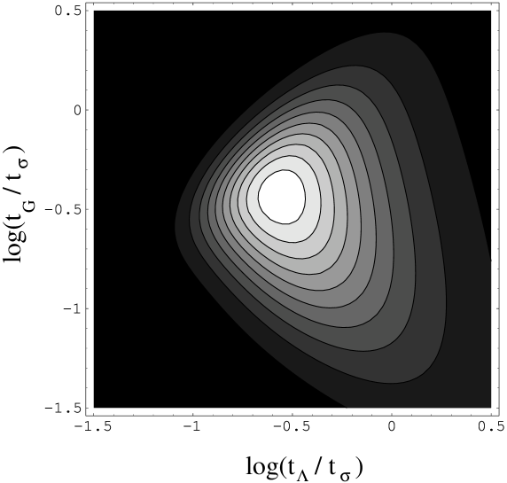
FIG. 2.: The joint probability density (15) per unit area in the plane $\log\ (t_{\Lambda}/t_{\sigma})$ (horizontal axis) $\log(t_{G}/t_{\sigma})$ (vertical axis), where $t_{\sigma}$ is defined in Eq. (16).

III Why Now?

As we noted in the Introduction, one of the most puzzling aspects of the value of $\Omega_{\Lambda}$ is related to the fact that the coincidence $t_{0}\sim t_{\Lambda}$ appears to be implying that we live in a special time. A similar problem exists even if a quintessence component [21] is assumed (see Section V). As we have shown in Section II, the epoch when giant galaxies are assembled, $t_{G}$, is expected to roughly coincide with the epoch of cosmological constant dominance, $t_{\Lambda}$. Therefore, if we could explain why $t_{0}\sim t_{G}$, the puzzle of the cosmic age coincidence would be resolved.

Most of carbon-based life may be expected to have appeared in the universe around the peak in the universal carbon production rate, at $t_{\rm carbon}$. The main contributors to carbon in the interstellar medium are stars in the mass range 1–2 M_⊙, through carbon stars and planetary nebulae [22]. Consequently, detailed simulations [23] show that the peak in the cosmic carbon production rate is delayed only by less than a billion years compared to the peak in the cosmic star formation rate, $t_{\rm SFR}$, namely,

$$t_{\rm carbon}\sim t_{\rm SFR}~{}~{}.$$ (17)

The appearance of intelligent life is further delayed by no more than a fraction of the main sequence lifetime of stars in the spectral range mid-F to mid-K ( 5-20 Gyr; [23, 24]). Following the main sequence, the expansion and increase in luminosity of stars spells the end of the possible existence of a biosphere on planets. Only stars in the above spectral range are expected to have continuously habitable zones around them (namely, ensuring the presence of liquid water and the absence of catastrophic cooling by ${\rm CO_{2}}$ clouds on planetary surfaces; [26]). Thus we have

$$t_{\rm IL}\sim t_{\rm carbon}\sim t_{\rm SFR}~{}~{}.$$ (18)

The “present time” $t_{0}$ can be defined as the time when a civilization evolves to the point where it is capable of measuring the cosmological constant and becomes aware of the coincidence (1). The experience of our own civilization suggests that, on a cosmological timescale, this time is not much different from $t_{\rm IL}$,

$$t_{0}\approx t_{\rm IL}.$$ (19)

Carter [11] and others [12, 13] used the principle of mediocrity to argue that the lifetime of our civilization is unlikely to be much longer than the time it has already existed, that is, $\sim 10^{4}$ yrs. If we are typical, then this should be the characteristic lifetime of a civilization. This would imply that Eq. (19) is valid even if $t_{0}$ is understood as the time when any astronomical observations can be made. Carter’s argument has some force, but it is based on a single data point, and one may be reluctant to accept it, considering in particular its pessimistic implications. We note, however, that with our definition of $t_{0}$, Eq. (19) is likely to be valid regardless of the validity of Carter’s argument (that is, even if civilizations are likely to survive much longer than $t_{\rm IL}$). Combining (19) with (18), we have that for a typical civilization

$$t_{0}\sim t_{\rm SFR}.$$ (20)

Finally, models of galaxy formation in hierarchical clustering theories propose that Lyman-break galaxies (at $z\sim 3$) are the first objects of galactic size which experience vigorous star formation [27]. These objects therefore signal the onset of the epoch of galaxy formation, with cosmic star formation and galaxy formation being closely linked. In fact, the mergers and collisions of “sub-galactic” objects to produce galactic-size structures, are responsible for the enhanced star formation. In hierarchical models therefore

$$t_{G}\sim t_{\rm SFR}~{}~{}.$$ (21)

The above relation is also supported by observations of the star formation history, showing that the star formation rate rises from the present to about $z\sim 1$, with a broad peak (of roughly constant star formation rate) in the redshift range $z\sim 1$–3 [28]. This corresponds roughly to $t_{\rm SFR}\sim t_{0}/3$–$t_{0}/8$, in agreement with Eq. (21). In fact, more than 80% of the stars have already formed ($\Omega_{gas}/\Omega_{stars}\sim 0.18$ [29]).

Combining Eqs. (14),(20),(21) above we obtain the desired relation

$$t_{0}\sim t_{G}\sim t_{\Lambda}~{}~{}.$$ (22)

IV Models with variable $\Lambda$ and $\sigma_{rec}$

In the previous discussion we have assumed a fixed value of the density contrast at recombination $\sigma_{rec}$ (or equivalently, a fixed value of $Q$). This determines the parameter $t_{\sigma}\equiv(\Delta_{c}/\sigma_{rec})^{3/2}t_{rec}$ appearing in the distribution (15) and therefore, as it is clear from Fig. 2, the most probable time at which the cosmological constant will dominate $t_{\Lambda}\sim t_{\sigma}$ [6].

If $\sigma_{rec}$ is itself treated as a random variable, with a priori distribution ${\cal P}_{*}(\sigma_{rec})d\ln\sigma_{rec}$ then the most probable value of $t_{\Lambda}$ will of course have some dependence on ${\cal P}_{*}$. However, as we shall argue, this dependence is not too strong provided that ${\cal P}_{*}$ satisfies some qualitative requirements, in which case the most probable values of $t_{\Lambda}$ and $\sigma_{rec}$ are actually determined by the fundamental constants involved in the cooling processes which take place in collapsing gas clouds.

A The cooling boundary

So far, we have assumed that all the galactic-size objects collapsing at any time form luminous galaxies. However, galaxies forming at later times will have a lower density and shallower potential wells. They are thus vulnerable to losing all their gas due to supernova explosions [10]. Moreover, a collapsing cloud fragments into stars only if the cooling timescale of the cloud $\tau_{cool}$ is smaller than the collapse timescale $\tau_{grav}$. Otherwise, the cloud stabilizes into a pressure supported configuration [35, 10]. The cooling rate of such pressure supported clouds is exceedingly low, and it is possible that star formation in the relevant mass range will be suppressed in these clouds even when they eventually cool. Hence, it is conceivable that galaxies that fail to cool during the initial collapse give a negligible contribution to $\nu$. Fragmentation of a cloud into stars will be suppressed after a certain critical time which we shall refer to as the “cooling boundary” $t_{cb}$ [10].

To determine $t_{cb}$, let us first consider the case of a matter dominated universe (not necessarily flat) without a cosmological constant. An overdensity which is destined to collapse can be described in the spherical model as a part of a closed Friedmann-Robertson-Walker (FRW) universe. The size of this spherical region at the time of recombination is such that it basically contains the mass of a galaxy. The virialization temperature and the density after virialization will be quite independent of what happens outside the region, depending only on its gravitational energy at the time $t_{vir}$ when it collapses. The virial velocity will then be given by $v_{vir}\sim(GM_{g}/L)^{1/2}$, where $L$ is the size of the collapsing object at $t_{vir}$. The density of the virialized collapsing cloud $\rho_{vir}$ is given by [10, 36]

$$\rho_{vir}\sim 10^{2}(Gt_{vir}^{2})^{-1}.$$ (23)

The virialization temperature can be estimated as $T_{vir}\sim m_{p}v_{vir}^{2}\sim m_{p}(G^{3}\rho_{vir}M_{g}^{2})^{1/3}$. Here $m_{p}$ is the proton mass. The later an object collapses, the colder and more dilute it would be.

If there is a cosmological constant, then these estimates still hold to good approximation. Indeed, a spherical region will only collapse if its intrinsic “curvature” term is always dominant with respect to the cosmological constant term. The “potential” energy at the time of collapse and the properties of the virialized cloud will basically remain unaltered. In principle, a spherical region with a cosmological constant could enter a “quasistatic” phase where the gravitational pull is nearly balanced by the repulsion due to the cosmological constant. After a long period of time, this region might finally collapse and virialize to a large enough temperature. However, since the quasistatic phase is unstable we shall disregard this marginal possibility.

The cooling rate $\tau_{cool}^{-1}$ of a gas cloud of fixed mass depends only on its density and temperature, but as shown above both of these quantities are determined by $t_{vir}$ [39]. The timescale needed for gravitational collapse is $\tau_{grav}\sim t_{vir}$. Therefore, the condition $\tau_{cool}<\tau_{grav}$ gives an upper bound $t_{cb}$ on the time at which collapse occurs. Various cooling processes such as Bremsstrahlung and line cooling in neutral hydrogen and helium were considered in Ref. [10]. For a cloud of mass $M_{g}\approx 10^{12}M_{\odot}$, cooling turns out to be efficient [40] for

$$t<t_{cb}\approx 3\cdot 10^{10}{\rm yr}.$$ (24)

In any case, this value of $t_{cb}$ should be taken only as indicative, since the present status of the theory of star formation does not allow for very precise estimates.

B Likely values of $t_{\Lambda}$

Let us now consider the probability distribution for the three independent variables $x,x_{rec}$ and $\sigma_{rec}$. This will be proportional to the number of galaxies forming at a time charachterized by $x$ in a region with given values of $\sigma_{rec}$ and $x_{rec}$,

$$d{\cal P}(x,x_{rec},\sigma_{rec})\propto{\cal P}_{*}(\sigma_{rec})\exp\left[-{1\over 2}\left({\Delta_{c}\over F}{x^{1/3}_{rec}\over\sigma_{rec}}\right)^{2}\right]{F^{\prime}\over F^{2}}{x^{1/3}_{rec}\over\sigma_{rec}}dx\ dx_{rec}\ d\ln\sigma_{rec}.$$ (25)

Let us assume for simplicity a power-law a priori distribution,

$${\cal P}_{*}(\sigma_{rec})\propto\sigma_{rec}^{-\alpha},$$ (26)

where $\alpha$ is a constant. Then we can immediately integrate over $\sigma_{rec}$ and obtain

$$d{\cal P}(x,x_{rec})\propto x_{rec}^{-\alpha/3}F^{\alpha-1}F^{\prime}\ dx\ dx_{rec}.$$ (27)

Now we can integrate with respect to the “time” $x$ at which galaxies assemble, from the time of recombination $x_{rec}$ to the cooling boundary

$$x_{cb}=\sinh^{2}(t_{cb}/t_{\Lambda}).$$ (28)

The integral is simply the difference in $F^{\alpha}$ between the two boundaries in the integration range, and we shall neglect the contribution at $x_{rec}$. Finally, using $t_{\Lambda}=t_{rec}x_{rec}^{-1/2}$ we obtain a probability distribution for $t_{\Lambda}$

$$d{\cal P}(t_{\Lambda})\propto F^{\alpha}(\sinh^{2}(t_{cb}/t_{\Lambda}))t_{\Lambda}^{{2\alpha\over 3}-2}d\ln(t_{\Lambda}/t_{cb}).$$ (29)

Thus, the most probable value of $t_{\Lambda}$ is determined by $t_{cb}$ and $\alpha$.

In Fig. 3, this distribution is plotted for different values of $\alpha$ ranging from 4 to 15. In all these cases we have

$$t_{\Lambda}\sim t_{cb}.$$ (30)

The behaviour of the distribution is different for $\alpha\leq 3$. Note that $F(y)\propto y^{1/3}$ for small y, whereas $F$ saturates at a constant value for large $y$. This means that if $\alpha<3$, the distribution (29) would favour very small values of $t_{\Lambda}$. The reason is that for a small $\alpha$ the a priori distribution is not too suppressed at large $\sigma_{rec}$, and it pays off to increase $\sigma_{rec}$ in order to obtain a large number of collapsed objects very soon after recombination. Therefore the time of $\Lambda$ domination can be very short without interfering with galaxy formation. Of course, this would result in an overwhelming majority of the galaxies in regions which do not look anything like ours. On the other hand, if $\alpha>3$, small values of $\sigma_{rec}$ are preferred. However, the value of $\sigma_{rec}$ should at least be large enough for galaxy formation to occur marginally before the cooling boundary $t_{cb}$. Therefore, if the cosmological constant is not to interfere with galaxy formation, the result (30) is expected. More generally, we expect the relation (30) to be valid if the a priori distribution decreases faster than $\sigma_{rec}^{-3}$ at small $\sigma_{rec}$. With $t_{cb}$ from Eq. (24) and the $t_{\Lambda}$ suggested by observations, the relation (30) is indeed satisfied.

FIG. 3.: The probability density per unit logarithmic interval of $t_{\Lambda}/t_{cb}$, Eq. (29), for different values of the parameter $\alpha$ ($\alpha=4,5,10,$ and $15$).

C Likely values of $\sigma_{rec}$

A probability distribution for $\sigma_{rec}$ can be obtained by integrating (25) first over $x_{rec}$ over the relevant range $\sinh(x_{rec}^{1/2}t_{cb}/t_{rec})>x^{1/2}$, and then over $x$. The result can be expressed as

$$d{\cal P}(\beta)\propto\beta^{2(\alpha-3)/3}G(\beta)\ d\ln\beta,$$ (31)

where we have introduced the $\sigma_{rec}$ dependent parameter

$$\beta={t_{\sigma}\over t_{cb}}=\left({\Delta_{c}\over\sigma_{rec}}\right)^{3/2}{t_{rec}\over t_{cb}}$$ (32)

and the function

$$G(\beta)=\int_{0}^{\infty}\exp\left[-{1\over 2F^{2}}\left({\beta t\over t_{\Lambda}}\right)^{4/3}\right]F^{\prime}\left[F^{2}+{1\over 2}\left({\beta t\over t_{\Lambda}}\right)^{4/3}\right]dx.$$ (33)

The function $G(\beta)$ is plotted in Fig. 4 (thick solid line). It stays constant for $\beta<1$ (towards large $\sigma_{rec}$) and it drops to zero around $\beta\approx 10$. For larger $\beta$ it falls off as $\beta^{4/3}\exp(-\beta^{4/3}/2)$. This function is multiplied in (31) by the factor $\sigma_{rec}^{3-\alpha}$, which depends on the a priori distribution for $\sigma_{rec}$. If this factor is a decreasing function of $\sigma_{rec}$ (i.e. $\alpha>3$) then (31) peaks between $1<\beta\lesssim 10$. This is illustrated in Fig. 4 (thin curves) for $\alpha=4$ and $5$. From the definition of $\beta$ we have

$$\sigma_{rec}={\Delta_{c}\over(1+z_{rec})}\left({2\over 3\beta H_{0}t_{cb}\sqrt{\Omega_{M}}}\right)^{2/3}\approx 1.1\cdot 10^{-3}\beta^{-2/3}.$$ (34)

Here, we have used the relation $Hx^{1/2}=2/(3t_{\Lambda}\sqrt{\Omega_{M}})$, where all quantities (including the matter density parameter $\Omega_{M}$) are evaluated at the present time, and for our numerical estimate we have taken $z_{rec}=1000$, $t_{cb}=3\cdot 10^{10}yr$, $H_{0}=100\ h\ km\ s^{-1}\ Mpc^{-1}$, with $h=.7$, and $\Omega_{M}=.3$. For $\beta\sim 1$, as suggested by the distribution (31), we have that the most likely values of $\sigma_{rec}$ are of the order of $10^{-3}$. This is close to the observationally suggested values $\sigma_{rec}=(3.3-2.4)10^{-3}$ [6].

FIG. 4.: The probability density per unit logarithmic interval of $\beta\propto\sigma_{rec}^{-3/2}$, Eq. (31), for $\alpha=4$ and $5$ (thind solid lines). The function $G(\beta)$ is represented by a thick solid line.

Anthropic bounds on the density contrast have been recently discussed by Tegmark and Rees [10]. Instead of $\sigma_{rec}$, they used the amplitude of the density fluctuations at horizon crossing, $Q$; the relation between the two is roughly $Q\sim 10^{-2}\sigma_{rec}$. They imposed a lower bound on $Q$ by requiring that galaxies form prior to the “cooling boundary”, $t_{\sigma}\lesssim t_{cb}$. This gives $Q\gtrsim 10^{-6}$. To obtain an upper bound, it has been argued [30, 10] that for large values of $Q$ galaxies would be too dense and frequent stellar encounters would disrupt planetary orbits. To estimate the rate of encounters, the relative stellar velocity was taken to be the virial velocity $v_{vir}\sim 200~{}km~{}s^{-1}$, resulting in a bound $Q\lesssim 10^{-4}$. However, Silk [31] has pointed out that the local velocity dispersion of stars in our Galaxy is an order of magnitude smaller than $v_{vir}$. This gives $Q\lesssim 10^{-3}$, which is a rather weak constraint. This issue does not arise in the approach we take in the present paper, since in our case large values of $Q$ are suppressed by the a priori distribution ${\cal P}_{*}(\sigma_{rec})$.

D The time coincidence

Finally, we should check that the introduction of a cooling boundary does not spoil the coincidence $t_{G}\sim t_{\Lambda}$. In fact, this seems rather clear from Fig. 2. Introducing the cooling boundary basically amounts to disregarding the probability density above a certain horizontal line $t_{G}=t_{cb}$. The probability distribution for $t_{G}/t_{\Lambda}$ below the horizontal line is somewhat different from that in the whole plane, but clearly it still peaks around $t_{G}\sim t_{\Lambda}$. To quantify this effect, we have integrated (12) with respect to $x_{rec}$ over the range $\sinh(x_{rec}^{1/2}t_{cb}/t_{rec})>x^{1/2}$. The resulting distribution for $x$ is proportional to the integrand in the right hand side of (33). For $\beta=2$, this probability density is shown in Fig. 1 (curve $b$). The peak is only slightly shifted towards smaller values of $t_{G}/t_{\Lambda}$.

Cooling failure is not the only mechanism that can in principle inhibit the number of civilizations at low $\sigma_{rec}$. It is possible, for example, that the stellar initial mass function (IMF) depends on the protogalactic density $\rho_{vir}$, so that the number of carbon forming stars drops rapidly towards very low values of $\rho_{vir}$. If the a priori distribution ${\cal P}_{*}(\sigma_{rec})$ is a decreasing function of $\sigma_{rec}$, this can result in a peaked distribution $d{\cal P}/d\ln t_{\Lambda}$. Quite similarly, if the number of relevant stars grows towards smaller $\rho_{vir}$, a peaked distribution is obtained for an increasing function ${\cal P}_{*}(\sigma_{rec})$. Our present understanding of star formation is insufficient to determine the dependence of the IMF on $\rho_{vir}$, but once it is understood, the probability distribution for $t_{\Lambda}$ can be calculated as outlined above [32].

V Conclusions

In this paper we suggested a possible explanation for the near-coincidence of the three cosmological timescales: the time of galaxy formation $t_{G}$, the time when the cosmological constant starts to dominate the energy density of the universe $t_{\Lambda}$, and the present age of the universe $t_{0}$. Since this coincidence involves specifically the time of our existence as observers, it lends itself most naturally to the consideration of anthropic selection effects.

We considered a model in which the cosmological constant is a random variable with a flat a priori probability distribution. We showed that a typical galaxy in this model forms at a time $t_{G}\sim t_{\Lambda}$. We further demonstrated that a typical civilization should determine the value of the cosmological constant at $t_{0}\sim t_{G}$. Thus we should not be surprised to find ourselves discussing the cosmic time coincidence.

We also considered a model in which both the cosmological constant $\Lambda$ and the density contrast $\sigma_{rec}$ are random variables. The galaxy formation in this case is spread over a much wider time interval, and we had to account for the fact that the cooling of protogalactic clouds collapsing at very late times is too slow to allow for efficient fragmentation and star formation. We therefore disregarded all galaxies formed after the “cooling boundary” time $t_{cb}$. We assumed that the a priori distribution for $\sigma_{rec}$ is a decresing power law and found that, for a sufficiently steep power, a typical observer detects $\sigma_{rec}\sim 10^{-3}-10^{-4}$, close to the values inferred from observations. Such observers are likely to find themselves living at $t_{0}\sim t_{\Lambda}$ in a galaxy formed at $t_{G}\sim t_{\Lambda}$ in a region of the universe where $t_{\Lambda}\sim t_{cb}$, also close to the observationally suggested value.

Our model with variable $\Lambda$ and $\sigma_{rec}$ can be developed further in several directions. Instead of taking a flat distribution for $\rho_{\Lambda}$ and a power-law distribution for $\sigma_{rec}$, one could use the methods of Refs. [17, 38] to calculate the a priori distributions for these variables in the framework of some inflationary model. One could also use a more refined model of structure formation and improve on our treatment of cooling failure, replacing the sharp cutoff at $t=t_{cb}$ with a more realistic model. We believe, however, that even in the present, simplified form our model indicates that an anthropic selection for $\Lambda$ and $\sigma_{rec}$ is a viable possibility.

Finally, we should note that the coincidence in the timescales requires an explanation even in models involving a quintessence component [21]. In models of quintessence the universe at late times is dominated by a scalar field $\phi$, slowly evolving down its potential $V(\phi)$. It has been argued (by Zlatev et al. [37]) that such models do not suffer from the cosmic time coincidence problem, because the time $t_{\phi}$ of $\phi$-domination is not sensitive to the initial conditions. This time, however, does depend on the details of the potential $V(\phi)$, and observers should be surprised to find themselves living at the epoch when quintessence is about to dominate. More satisfactory would be a model in which the potential depends on two fields, say $\phi$ and $\chi$, with $\chi$ slowly varying in space, making the time of $\phi$-domination position dependent. Such models are not difficult to construct in the context of inflationary cosmology. One could then apply the principle of mediocrity to determine the most likely value of $t_{\phi}$.

Acknowlegements

We are grateful to Ken Olum for his comments on the manuscript. J.G. acknowledges support from CIRIT grant 1998BEAI400244. M.L. acknowleges support from NASA Grant NAG5-6857. A.V. was supported in part by the National Science Foundation.

Appendix: The probability distribution for $\Lambda$

In this Appendix we briefly discuss the probability distribution for the cosmological constant, giving a simplified version of the calculation presented in [6].

In a universe where the cosmological constant is non-vanishing, a primordial overdensity will eventually collapse provided that its value at the time of recombination exceeds a certain critical value $\delta^{rec}_{c}$. In the spherical collapse model this is estimated as $\delta^{rec}_{c}=1.13\ x_{rec}^{1/3}$ (see e.g. [41]). Hence, the fraction of matter that eventually clusters in galaxies can be roughly approximated as [20, 41]:

$$\nu(x_{rec})\approx{\rm erfc}\left({\delta^{rec}_{c}\over\sqrt{2}\sigma_{rec}(M_{g})}\right)\approx{\rm erfc}\left({.80\ x_{rec}^{1/3}\over\sigma_{rec}(M_{g})}\right).$$ (35)

Here, erfc is the complementary error function and $\sigma_{rec}(M_{g})$ is the dispersion in the density contrast at the time of recombination on the relevant galactic mass scale $M_{g}\sim 10^{12}M_{\odot}$. The logarithmic distribution $d{\cal P}/d\ln\ x_{rec}=x_{rec}\nu(x_{rec})$ is plotted in Fig. 5. It has a rather broad peak which spans two orders of magnitude in $x_{rec}$, with a maximum at

$$x^{peak}_{rec}\approx 2.45\ \sigma_{rec}^{3}.$$ (36)

In accordance with the principle of mediocrity, we should expect to measure a value of the cosmological constant within this broad peak of the distribution. And indeed, this may actually be the case. The distribution (35) is characterized by the parameter $\sigma_{rec}$. As noted by Martel et al. [6], this parameter can be inferred from observations of the cosmic microwave background anisotropies, although its value depends on the assumed value of the cosmological constant today. For instance, assuming that the present cosmological constant is $\Omega_{\Lambda,0}=.8$, and the relevant galactic co-moving scale is in the range $R=(1-2)Mpc$, Martel et al. found $\sigma_{rec}=(2.3-1.7)\ 10^{-3}$. In this estimate, they also assumed a scale invariant spectrum of density perturbations, a value of $70km\ s^{-1}\ Mpc^{-1}$ for the present Hubble rate, and they defined recombination to be at redshift $z_{rec}\approx 1000$ (this definition is conventional, since the probability distribution for the cosmological constant does not depend on the choice of reference time). Thus, taking into account that $x$ scales like $(1+z)^{-3}$ in equation (36), one finds that the peak of the distribution for the cosmological constant today is at $x_{0}^{peak}\approx 29.8-12$. The value corresponding to the assumed $\Omega_{\Lambda,0}=.8$ is $x_{0}=4$, certainly within the broad peak of the distribution and not far from its maximum. If instead we assume that the measured value is $\Omega_{\Lambda,0}=.7$, which corresponds to $x_{0}=2.33$, the new inferred values for $\sigma_{rec}$ correspond to the peak value $x_{0}^{peak}\approx(88-34)$. In this case, the measured value would be at the outskirts of the broad peak, where the logarithmic probability density is about an order of magnitude smaller than at the peak, but still significant. Thus, even though there may be uncertainties in the inferred value of $\sigma_{rec}$ on the relevant scales, it seems fair to say that any observed value of $\Omega_{\Lambda,0}\gtrsim.7$ is in good agreement with the principle of mediocrity.

FIG. 5.: The probability density per unit logarithmic interval of $x_{rec}\sigma_{rec}^{-3}$.

REFERENCES

- [1] S. Perlmutter et al., Ap.J. 483, 565 (1997); S. Perlmutter et al., astro-ph/9812473 (1998); B. Schmidt et al., Ap.J. 507, 46 (1998); A. J. Riess et al., A.J. 116, 1009 (1998).
- [2] P. S. Drell, T. J. Loredo and I. Wasserman, preprint (1999); M. Livio, in Type Ia Supernovae: Theory and Cosmology (Cambridge University Press, Cambridge, UK, 1999).
- [3] M. S. Turner, Pub. Astron. Soc. Pac., in press (1999) (astro-ph/9811454) and references therein; G. Efstathiou et al., (1998) (astro-ph/9812226).
- [4] A.Vilenkin, Phys. Rev. Lett. 74, 846 (1995).
- [5] S. Weinberg, in Critical Dialogues in Cosmology, ed. by N. G. Turok (World Scientific, Singapore, 1997).
- [6] H. Martel, P. R. Shapiro and S. Weinberg, Ap.J. 492, 29 (1998).
- [7] For a related approach see also G. Efstathiou, M.N.R.A.S. 274, L73 (1995).
- [8] A. Vilenkin and S. Winitzki, Phys. Rev. D55, 548 (1997).
- [9] J. Garriga, T. Tanaka and A. Vilenkin, astro-ph/9803268.
- [10] M. Tegmark and M. J. Rees, Ap.J. 499, 526 (1998).
- [11] B. Carter, unpublished.
- [12] J. Leslie, Mind 101.403, 521 (1992).
- [13] J.R. Gott, Nature 363, 315 (1993).
- [14] A. D. Linde, D. A. Linde, and A. Mezhlumian, Phys. Rev. D49, 1783 (1994). J. Garcia-Bellido, A.D. Linde and D.A. Linde, Phys. Rev. D50, 730 (1994); J. Garcia-Bellido and A.D. Linde, Phys. Rev. D51, 429 (1995).
- [15] A. Albrecht, in Lecture Notes in Physics, Springer-Verlag, Berlin, 1995.
- [16] For a review of inflation, see, e.g., A.D. Linde, Particle Physics and Inflationary Cosmology (Harwood Academic, Chur, Switzerland, 1990).
- [17] A. Vilenkin, Phys. Rev. Lett. 81, 5501 (1998).
- [18] S. Weinberg, Phys. Rev. Lett. 59, 2607 (1987).
- [19] A similar argument for the coincidence of the galaxy formation time with the curvature domination time in models of open inflation was given in Ref.[9].
- [20] W.H. Press and P. Schechter, Astrophys. J. 187,425 (1974).
- [21] P.J.E. Peebles and B. Ratra, Ap. J. Lett. 325, L17 (1988); R.R. Caldwell, R. Dave and P.J. Steinhardt, Phys. Rev. Lett. 80, 1582 (1998).
- [22] I. Iben, Jr. and A. Renzini, Ann. Rev. Astron. Ap. 21, 271 (1983); J. B. Kaler and G. H. Jacoby, Ap.J. 382, 134 (1991); G. Wallerstein and G. R. Knapp, Ann. Rev. Astron. Ap. 36, 369 (1998).
- [23] M. Livio, Ap.J. 511, 429 (1999).
- [24] In fact, for a Salpeter initial mass function [25] and under simple assumptions, the highest probability for the time to evolve an intelligent civilization, , lies in the neighborhood of the Sun’s lifetime [23].
- [25] E.E. Salpeter, Ap.J. 121, 161 (1955).
- [26] J. F. Kasting, D. P. Whitmore and R. T. Reynolds, Icarus 101, 108 (1993).
- [27] C. M. Baugh, S. Cole, C. S. Frenk and C. G. Lacey, Ap.J. 498, 504 (1998).
- [28] S. J. Lilly, O. Le Fèvre, F. Hammer and D. Crampton, Ap.J. 460, L1 (1996); P. Madau, H. C. Ferguson, M. E. Dickinson, M. Giavalisco, C. C. Steidel and A. Fruchter, Mon. Not. R. Astr. Soc. 283, 1388 (1996); C. C. Steidel, K. L. Adelberger, M. Giavalisco, M. Dickinson and M. Pettini, astro-ph/9811399 (1998).
- [29] M. Fukugita, C.J. Hogan and P.J.E. Peebles, Ap. J. 503, 518 (1998).
- [30] A. Vilenkin, Talk given at the 1st RESCEU Symposium, Tokyo (1995).
- [31] J. Silk, Private communication.
- [32] There exist some indications that the IMF may depend on density. For example, it has been suggested that the IMF is biased towards high masses in very active regions like starbursts [33], and towards low masses in regions of extreme inactivity, like the field population [34]. These suggestions are not very certain because the observations are influenced by selection effects and by evolution.
- [33] G.H. Rieke, M.J. Lebofsky, R.I. Thompson, F.J. Low and A.T. Tokunaga, Ap. J. 238, 24 (1980).
- [34] P. Massey, C.C. Lang, K. DeGioia - Eastwood and C.D. Garmany, Ap. J. 438, 188 (1995).
- [35] M.J. Rees and J.P. Ostriker, MNRAS, 179, 541 (1977); J. Silk, ApJ., 211, 638 (1977).
- [36] C. Lacey and S. Cole, MNRAS, 262, 627 (1993).
- [37] I. Zlatev, L. Wang and P.J. Steinhardt, Phys. Rev. Lett. 82, 896 (1999).
- [38] V. Vanchurin, A. Vilenkin and S. Winitzki, gr-qc/9905097.
- [39] Actually, the fraction of baryonic matter is also relevant for cooling. Following [10] we shall take .
- [40] This upper bound on is determined by line cooling in Helium. For there is also a narrow interval near , where cooling is again efficient due to hydrogen line cooling. However, the interval is very narrow and we shall disregard the galaxies which may form during this short late period.
- [41] H. Martel and P.R. Shapiro, astro-ph/9903425.