Molecular gas associated with the IRAS-Vela shell

Abstract

We present a survey of molecular gas in the J = 1$\rightarrow$ 0 transition of ¹²CO towards the IRAS Vela shell. The shell, previously identified from IRAS maps, is a ring-like structure seen in the region of the Gum Nebula. We confirm the presence of molecular gas associated with some of the infrared point sources seen along the Shell. We have studied the morphology and kinematics of the gas and conclude that the shell is expanding at the rate of $\sim$ 13 km s^-1from a common center. We go on to include in this study the Southern Dark Clouds seen in the region. The distribution and motion of these objects firmly identify them as being part of the shell of molecular gas. Estimates of the mass of gas involved in this expansion reveal that the shell is a massive object comparable to a GMC. From the expansion and various other signatures like the presence of bright-rimmed clouds with head-tail morphology, clumpy distribution of the gas etc., we conjecture that the molecular gas we have detected is the remnant of a GMC in the process of being disrupted and swept outwards through the influence of a central OB association, itself born of the parent cloud.

1 Introduction

The IRAS Vela Shell is a ring-like structure seen clearly in the IRAS Sky Survey Atlas (ISSA) in the 25, 60 and 100 micron maps. This large feature extending almost 30 degrees in Galactic longitude ($l^{\rm II}=245^{\circ}$ to $275^{\circ}$), and discernable from the galactic plane till galactic latitude $-15^{\circ}$, was first noticed by A. Blaauw. Subsequently, a detailed study of this region formed the major part of the thesis by Sahu (1992). This infrared shell is seen in projection against the Gum Nebula as a region of enhanced H$\alpha$ emission in the southern part of the nebula. But it is quite likely that whereas the IRAS shell may be located in the vicinity of the Gum Nebula, it is unrelated to it. The main reason for supposing this is that the kinematics of the shell is quite different from that of the Gum Nebula as a whole. The evidence comes from emission line studies of this region (e.g., lines of NII). Whereas there is no conclusive evidence of any expansion of the Gum Nebula, in two directions towards approximately the centre of the shell the emission lines have a “double-peaked” structure, consistent with an expansion with a velocity $\sim 10\pm 2\;\;{\rm km\;s}^{-1}$. Moreover, the Gum Nebula does not appear as a discernable feature in the IRAS maps.

The shell roughly envelopes the Vela OB2 stellar association (Brandt et al. 1971). Two of the brightest known stars, $\zeta$ Puppis (spectral type 04If) and $\gamma^{2}$ Velorum a Wolf-Rayet binary are also located close to the shell on the sky. Based on the symmetric location of the shell with respect to the Vela OB2 association, Sahu argued that this group of stars is associated with the shell. The distance estimate to Vela OB2 association is $\sim 450\;{\rm pc}$, and this has been taken as the distance to the shell as well (Sahu, 1992).

The IRAS Point Source Catalogue (IPSC) also reveals a ring-like structure, although slightly offset in position from the ISSA shell. From its emissivity in the infrared, and assuming the standard $1:100$ ratio of dust to gas, Sahu estimated the total mass of the shell to be $\sim 10^{6}$ solar masses. Presumably much of this mass must be in the form of molecular gas. The only evidence for this so far is restricted to the $\sim$ 35 or so cometary globules in the region. These, with head-tail structures, are distributed in the region of the shell in a manner which suggests a physical association. From a comprehensive study of these globules Sridharan (1992a,b) concluded that these small molecular clouds are expanding about a common centre with a velocity $\sim$ 12 km s^-1. It turns out that this centre of expansion is roughly centred on the infrared shell as delineated by the IRAS point sources. This strengthens the case for the cometary globules being associated with the IRAS Vela Shell. Even so, this would account for only a few thousand solar masses of molecular gas since the mass of each of the globules is less than $\sim 100M_{\odot}$ (Sridharan, 1992b).

Figure 1: Overall picture of the Gum-Vela region showing the H$\alpha$ emission as solid lines, the cometary globules as filled circles with tails (scaled up 10 times for clarity), and other important objects in the region. The morphological centre of the system of cometary globules is indicated by a $+$ sign. From Sridharan (1992b).

The main objective of the investigation reported in this paper was to make an extensive survey for molecular gas possibly associated with the IRAS shell. A second objective was to study the kinematics of this gas. For future reference we show in figure 1 a schematic of the Gum-Vela region, and in figure 2 the distribution of the IRAS point sources.

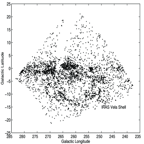
Figure 2: IRAS Point Sources between l = 240^∘ and l = 280^∘. These sources satisfy the criteria for Young Stellar Object candidates listed in the text. The IRAS Vela Shell is noticeable below the Galactic plane.

2 Source Selection

In order to increase our chances of detecting molecular gas we chose a sample of point sources in the IPSC which were candidates for Young Stellar Objects (YSO); it had been noted by earlier workers that the shell-like structure in the distribution of the IRAS point sources was more pronounced if one restricted oneself to those which are likely to be associated with YSOs. Prusti (1992), for example, used a certain “Classifier III” criteria to pick out the YSO candidates in the IPSC. In addition to colour and statistical criteria Prusti used certain “crowding” properties which tended to enhance the “shell-structure”. Since the use of such a filter would excessively bias the distribution of sources selected for our survey, we used instead a less restrictive criteria used by Sridharan (1992b), and which are originally due to Emerson (1987) and Parker (1988). These are listed below:

1. Detection at $25\mu m$ and $60\mu m$, with $[60-25]>0$.

2. $[25-12]>0$, if also detected at $12\mu m$.

3. Detection only at $60\mu m$.

4. Detection at $60\mu m$ and $100\mu m$ only with $[100-60]>0.6$.

5. $[100-25]>0.$

Here the notation $[25-12]$, for example, refers to the 25 to $12\mu m$ colour ratio, defined to be $\log\left[S_{25}/S_{12}\right]$. The flux density in Jansky at $25\mu m$ is denoted by $S_{25}$, etc.. We used the filter specified above on the IPSC sources in the RA range 7 hours to 9 hours which covers the Shell (see figure 2).

3 The observations

In March–April 1996 we undertook millimeter-wave observation in the $J=1\rightarrow 0$ rotational transition of the ${}^{12}{\rm CO}$ molecule at $115.271$ GHz. The observations were done with the 10.4 m telescope located in the campus of the Raman Research Institute. It has an altitude-azimuth mount with the receiver at the Nasmyth focus. The receiver is a Schottky diode mixer cooled to 20 K. Further details about the telescope and the subsystems may be found in Patel (1990). The backend used was a hybrid type correlation spectrometer configured for a bandwidth of 80 MHz with 800 channels giving a resolution of $\approx 100\;{\rm kHz}$ when using both polarizations. This corresponds to a velocity resolution of $0.26\;\;{\rm km\;s}^{-1}$.

The observations were done in the frequency switched mode. This had the advantage that no time is spent looking at source-free regions. Moreover, since our sources were not point sources “off-source” regions are not well defined for beam switching schemes. A frequency offset of $15.25$ MHz was chosen between ON and OFF spectra since that is the frequency of the observed baseline ripple. With this scheme only a polynomial fit was required to remove any residual baseline curvature. The switching rate was 2 Hz. Calibration was done using an ambient temperature load at intervals of several minutes. The pointing error was within $20"$ (as determined by observing Jupiter). The frequency stability of the correlator was checked by observing the head of the cometary globule CG1 each day. The rms of this distribution was $0.3\;\;{\rm km\;s}^{-1}$, and hence that will be the error on the velocities quoted by us. A comparison of the velocities measured by us towards the heads of several cometary globules with those measured by Sridharan (1992b) showed good agreement.

Figure 3: A typical spectrum showing ¹²CO emission (J = 1$\rightarrow$ 0 transition, $\lambda$ = 2.6mm, $\nu_{0}$ = 115.271 GHz) after removal of a polynomial fit to the baseline. The spectrum was obtained towards the IRAS point source IR 56549 in the Shell. The vertical axis shows T_A${}^{\thinspace*}$ (calibrated antenna temperature) in K. The effective integration time was $\sim$ 20 minutes.

Due to the limited observing season we selected about 100 IPSC sources out of about 3750 which satisfied the various criteria mentioned before. The sources selected for observations covered the shell although not uniformly. In addition, we observed in several directions (within the shell) where there were no IPSC sources. Each observing run consisted of typically ten minutes of integration. The spectra in the vertical and horizontal polarizations were then averaged after removing the baseline curvature. The effective integration time was therefore typically $\sim 20$ minutes. The rms of the noise over such an integration period was $\sim 0.2\;{\rm K}$. In figure 3 we show a typical spectrum after correcting for the baseline curvature. The reduction of the data was done using the UNIPOPS package. The temperature scale T${}_{\rm A}^{\thinspace*}$ is telescope dependent but we shall not convert it to an absolute scale since in this paper we are only interested in detection (or otherwise), and the velocities if molecular material is detected.

4 Results

We detected ${}^{12}{\rm CO}$ emission towards 42 of the 100 or so sources observed. Table 1 lists the measured antenna

Source	Vlsr	TA${}^{\thinspace*}$	Trms	Source	Vlsr	Ta∗	Trms
	km s-1	K	K		km s-1	K	K
51704	-1.2	0.6	0.12	61322	8.4	2.2	0.22
52594	-2.5	0.9	0.18	61322	13.2	1.5	0.22
53668	-0.5	0.5	0.13	61351	8.1	1.2	0.26
53829	-3.4	0.4	0.13	61428	7.7	3.0	0.14
54473	-1.2	0.8	0.18	61837	3.0	4.6	0.20
54599	-2.2	3.3	0.23	62100	9.9	7.7	0.12
54769	-3.1	1.7	0.13	62578	14.9	0.6	0.15
55878	-5.0	4.5	0.13	62717	3.9	3.3	0.21
55884	4.4	2.8	0.18	62841	-1.0	2.1	0.45
55925	5.5	0.9	0.24	62847	5.4	0.7	0.17
55932	21.5	0.8	0.14	63338	14.4	0.7	0.17
56549	2.2	3.6	0.27	63338	9.4	1.9	0.17
56831	-1.5	1.2	0.17	63927	4.6	1.4	0.20
57035	16.4	1.5	0.16	64029	8.8	3.7	0.16
57035	28.6	1.9	0.16	64154	14.1	1.4	0.16
57898	1.4	5.2	0.37	64388	0.9	2.2	0.14
58784	-8.2	1.1	0.18	64728	10.6	1.2	0.27
58793	8.6	0.3	0.12	64999	-4.0	1.1	0.25
58793	9.6	0.3	0.12	65728	7.0	2.4	0.27
59579	-7.5	0.9	0.24	65877	4.9	9.3	0.31
59584	5.7	0.8	0.18	66001	1.8	1.3	0.36
59891	-6.3	0.9	0.24	67910	6.0	3.3	0.30
60933	0.3	1.3	0.18	69185	3.5	2.0	0.30

Table 1: Summary of molecular detections toward IRAS Point Sources: Column 1 lists the IRAS Point Source Catalogue number for the source. Columns 2 and 3 give the LSR velocity and the corrected antenna temperature (see section 2.5). Column 4 gives the rms noise level for each source. The table is continued in Columns 5 to 8.

temperatures and LSR velocities found by fitting gaussians to the spectra. In some cases multiple features were detected at different velocities. The distribution of the observed sources in galactic coordinates is shown in figure 4; the circles denote detection of CO emission and the crosses indicate non-detections. While the distribution of the open circles suggests a ring-like structure it is not convincing. A gap in the distribution of detections in the lower right hand side of figure 4 is conspicuous. Interestingly, a number of cometary globules are located in this region. They, however, were not included in our sample selected from the IPSC. Since molecular gas has earlier been detected in these globules, their inclusion would fill in this gap (as we shall see in figure 5).

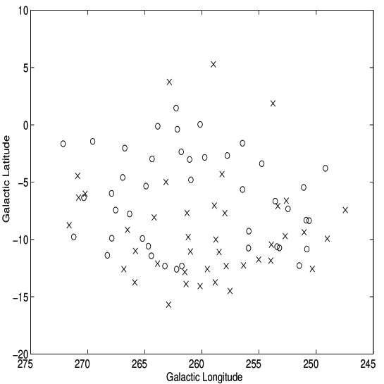
Figure 4: IPSC sources observed by us for CO emission are shown in Galactic coordinates. The circles denote detections and the crosses indicate non-detections. We have 42 detections from $\sim$ 100 pointings. The sensitivity limit was $\sim$ 0.6 K.

5 The kinematics of the molecular gas

In this section we wish to present an analysis of the kinematics of the molecular gas detected by us in the region of the IRAS Vela Shell. As already mentioned, there are two independent pieces of evidence to suggest that the shell-like structure may be in a state of expansion. To recall, the ionized gas possibly associated with the IRAS shell, as well as the cometary globules, both show evidence of expansion with a velocity $\sim 12\;\;{\rm km\;s}^{-1}$. If this is a general feature of the region under discussion then one would expect the more widely distributed molecular gas also to be in a state of expansion. Our analysis confirms this.

Sridharan’s study revealed that the system of cometary globules are expanding with the centre of expansion roughly coincident with the “morphological centre”, i.e., the point towards which the tails of the maximum fraction of the globules extrapolate to. This is located roughly at $l=260^{\circ}$ and $b=-4^{\circ}$. It is reasonable to assume that if the molecular gas detected by us is also expanding then it is likely to be with respect to the same “centre”. The analysis presented below is predicated on this assumption.

Figure 5: (a) A schematic for deriving expected radial velocities from an expanding shell. $V_{exp}$ is the expansion velocity, $V_{rad}$ is the radial component and $\Theta$ is the angular separation of any point on the shell from the center. (b) $V_{rad}$ plotted against (1$-sin^{2}\theta/sin^{2}\theta_{max})^{1/2}$.

Figure 5 illustrates the analysis procedure. The first step is to remove the contribution to the observed radial velocity due to the differential rotation of the Galaxy. Since we are looking for a possible expansion with respect to a common centre, we subtracted from the measured LSR velocity of each detection the radial velocity component at the assumed centre of expansion (viz. the morphological centre of the system of cometary globules) due to galactic differential rotation. The radial component of the rotation velocity was determined from the well known relation

$$v_{r}={\rm Ad}\sin 2l\cos^{2}b$$

As already mentioned,the co-ordinates of the assumed centre of expansion are $l=260^{\circ}$, $b=-4^{\circ}$. Following Kerr and Lynden-Bell (1986) we assumed a value of $14.5\;\;{\rm km\;s}^{-1}\;\;{\rm kpc}^{-1}$ for Oort’s constant $A$. As for the heliocentric distance $d$ to the centre of the shell, we adopted a value of 450 pc. This is consistent with the recent distance estimate to the Vela OB2 association based on the data from Hipparcos (de Zeeuw et al., 1997). It is also consistent with the distance estimate to the young star embedded in the head of the cometary globule CG1 (Brand et al., 1983).

It may be seen from figure 5 that if the objects expanding about the common centre with a velocity $v_{\rm exp}$ are distributed on a thin shell with a hollow interior then the residual radial velocity $v_{\rm res}$ (i.e., after allowing for galactic rotation) will be related to the expansion velocity by

$$v_{\rm res}=\pm\;v_{\rm exp}\left(1-\sin^{2}\theta/\sin^{2}\theta_{\rm max}\right)^{\frac{1}{2}}$$

where $\theta$ is the angular separation of the object from the centre of expansion, and $\theta_{\rm max}$ is (half) the angular size of the shell ($\sim 12.5^{\circ}$ in the present case). If the sources are distributed on a thin shell then in a plot of the residual radial velocity versus $\left(1-\sin^{2}\theta/\sin^{2}\theta_{\rm max}\right)^{\frac{1}{2}}$ the points would lie along two straight lines as shown in figure 5. If, on the other hand, the objects in question were distributed over the whole expanding volume then the points would lie within the envelope defined by the two lines (provided, of course, the inner objects are moving slower than the outer ones).

Figure 6: The residual radial velocity after removing the contribution from Galactic differential rotation plotted against the “expansion parameter” i.e., $(1-sin^{2}\theta/sin^{2}\theta_{max})^{1/2}$. $\theta$ is the angular separation of the source from the assumed center of expansion. If the objects form an expanding shell, the points will lie on the two straight lines (the “envelope”) shown. If they are distributed in a volume, the points would tend to lie within the envelope, as is the case here. The envelope in solid lines is for an expansion velocity of 13 km s^-1 with an offset of $-$3 km s^-1. The points are better “enclosed” by the solid lines than the envelope defined by the dashed lines (no offset).

Our data is shown in figure 6. In this plot we have included only those detections that are in the lower part of the shell (i.e. $b<0$) so as to avoid the confusing region near the galactic plane, for example, the Vela Molecular Ridge. Although its estimated distance of $\sim 1\;{\rm kpc}$ would put the Ridge well beyond the region under study here, there will be blending in velocity space towards these longitudes. As may be seen in the figure, the IRAS point sources (with which the molecular gas we have detected is associated) are expanding about a common centre. The filled nature of the cone suggests that the gas is not confined to a thin shell but rather distributed over a volume, with the outer regions expanding faster. From the slope of the two lines enveloping the data points we deduce that the outer regions are expanding with a velocity $\sim 13\;\;{\rm km\;s}^{-1}$. The data also suggests that there may be offset of $\sim-3\;\;{\rm km\;s}^{-1}$, i.e. the expansion is more symmetric with respect to a residual radial velocity of $-3\;\;{\rm km\;s}^{-1}$ than about zero velocity. If this is significant then it would imply that the gas has an overall drift. We shall return to this presently.

5.1 The southern dark clouds

It may be recalled that our search for molecular gas was motivated by a shell-like structure seen in the distribution of IRAS point sources. Indeed, our candidates were a sample of these point sources; due to the limited observing season at the site of the telescope we used we could only observe about 100 of these sources. Nevertheless, due to fortuitous circumstances, molecular observations of a different class of objects – some of which are possibly related to the feature we were investigating – became available to us. Recently a general survey of the population of dark clouds in the southern sky was undertaken in the $J=1\rightarrow 0$ line of ${}^{12}{\rm CO}$ using the Mopra antenna (Otrupcek, Hartley and Wang Jing-Sheng, 1995). These clouds listed in the Catalogue of Dark Clouds by Hartley et al. (1986) appear as dark patches of obscuration in optical photographs. Interestingly, the extinction map made from the ESO/SERC Southern Sky Survey by Feitzinger and Stüwe (1984) shows a shell-like structure just in the region of the IRAS shell. In view of this we decided to enlarge our database of molecular gas in the region of the IRAS shell by including the southern dark clouds. The radial velocities from the Mopra Survey were very kindly made available to us by Otrupcek.

Figure 7: The figure shows the molecular detections towards IRAS point sources (plus signs), and the Southern Dark Clouds including cometary globules in the region of the IRAS Vela Shell shown as open circles. The arrow indicates the morphological center of the cometary globule system.

In figure 7 we have replotted the molecular gas detected in this region, this time including the dark clouds, as well as the cometary globules. Since the molecular detections of the Soutern Dark Clouds is not yet published, we have given in the Appendix an extensive Table of the coordinates and measured LSR velocities of the subset of the Dark Clouds within the IRAS Vela Shell (i.e., within 12.5^∘ from the assumed centre of expansion). The corresponding data for the cometary globules were taken from Sridharan (1992b).In figure 7, the IRAS point sources observed by us are shown as plus signs, and the rest as open circles. The tip of the arrow represents the point with respect to which both the IRAS point sources as well as the cometary globules appear to be expanding. Since the distribution of the dark clouds also suggests a shell-like structure it is conceivable that they, too, are in a state of expansion. This is indeed the case. Figure 8 clearly shows that the molecular clouds associated with the young stellar objects in the region, the cometary globules, and a subset of the southern dark clouds are members of a common family, and that they are expanding with respect to a common centre.

Figure 8: The residual velocity plotted against $(1-sin^{2}\theta/sin^{2}\theta_{max})^{1/2}$ for all objects. The crosses denote SDCs, the open circles are cometary globules and the plus signs show molecular detections towards IPSC sources. The “expansion envelope” is for an expansion velocity of 13 km s^-1and offset of $-$3 km s^-1.

As in the analysis presented earlier in figure 6, to avoid confusion with unrelated objects near the galactic plane we have included only those dark clouds with latitudes greater than $-4^{\circ}$. We have, however, included all the cometary globules; in view of their distinctive morphology there is less chance of confusion.

5.2 A statistical test

To rule out the possibility that the signature of expansion seen in figure 8 is spurious we did the following test. It essentially involved scrambling the observed (residual) radial velocities among the objects in the sample, and determining the fraction of points which lie within the envelope defined by an expansion velocity $v_{\rm exp}$ and an offset $v_{\rm offset}$. For every assumed value of the ‘offset’ we determined the minimum value of $v_{\rm exp}$ for which $\geq 95\%$ of the observed points fell within the expansion envelope. Given a pair $\left(v_{\rm exp},v_{\rm offset}\right)$ so determined, we generated a large set of random samples and determined for each set the fraction of random samples that fall within the wedge-shaped region in figure 9 . If the mean of this distribution of fractions is not significantly different from the fraction of the actual observed sample that lies within the defined envelope, then the expansion deduced by us would not be statistically significant. The most statistically significant values we obtained were $v_{\rm exp}=13\;\;{\rm km\;s}^{-1}$ and $v_{\rm offset}=-3\;\;{\rm km\;s}^{-1}$. The results of 400,000 simulations for this pair of values is shown in figure 9 . As may be seen, one can say with a confidence at $3.3\sigma$ level that the observed radial velocities (after correcting for contribution from galactic rotation) indicates an expansion. For completeness we mention that we also did simulations for offsets of 1, 0, $-2$ and $-4\;\;{\rm km\;s}^{-1}$, all with $v_{\rm exp}=13\;\;{\rm km\;s}^{-1}$. As mentioned above, the most significant value for the offset in the residual velocity was $-3\;\;{\rm km\;s}^{-1}$, with the significance decreasing on either side of this value.

Figure 9: Result of significance tests done for an expansion velocity of 13 km s^-1 and offset of $-$3 km s^-1. In these tests, the velocity axis in the $V_{LSR}$ vs $(1-\sin^{2}\theta/\sin^{2}\theta_{max})^{1/2}$ diagram was “scrambled” and the number of points within the “expansion envelope” computed for each trial. The peak of the histogram shows the most likely fraction of points within the “expansion envelope” for a random sample. The arrow points to the fraction of points within the “expansion envelope” for the observed sample. This point lies 3.3 $\sigma$ away from the peak for the random samples.

6 Summary and discussion

We first summarize our main conclusions:

(i) There is a significant amount of molecular gas associated with the IRAS point sources defining the shell-like feature. Our observations thus confirm the expectation that molecular gas must be associated with these Young Stellar Objects.

(ii) Perhaps more importantly, these point sources which delineate the “IRAS Vela Shell” are expanding about a common centre, with the sources in the outer region moving with a velocity $\sim 13\;\;{\rm km\;s}^{-1}$.

(iii) Our study has established that a subset of the “Southern Dark Clouds” in this region are also part of this “shell” since they, too, are participating in the systematic motion mentioned above.

(iv) Earlier observers had found that the dozen or so cometary globules in this region, as well as some ionized gas, showed evidence of similar expansion with roughly the same velocity. One can therefore safely conclude that the cometary globules and the expanding ionized gas are also part of the “IRAS Vela Shell”.

6.1 The mass of the shell

We shall now attempt to estimate the mass of the shell. From its infrared emissivity Sahu (1992) estimated the amount of dust in the shell, and assuming the standard dust-to-gas ratio she estimated the mass of the shell to be $\sim 10^{6}M_{\odot}$. As we shall presently see, our estimates yield a mass an order of magnitude less than this.

As already discussed, the lower half $(b<-4^{\circ})$ of the IRAS Vela Shell is more clearly defined, and has an angular radius of $\sim 12.5^{\circ}$. Using the criteria explained earlier, we estimate that there are $\sim 1000$ Young Stellar Objects in the lower half of the shell. We shall now assume that these are of roughly the same mass as the typical cometary globules. The mass of a typical globule has been estimated to be $\leq 100M_{\odot}$ (Sridharan 1992b, and references therein). Adopting this value we estimate that the mass of the molecular gas associated with the entire IRAS Vela Shell must be $\sim 10^{5}M_{\odot}$. In deriving this estimate we have allowed for the fact that we detected molecular gas in only $\sim 50\%$ of the IPSC sources towards which we looked.

An alternative mass estimate can be made as follows. It has been argued that in the local giant molecular cloud complexes such as Orion, Ophiuchus and Taurus-Auriga the efficiency with which gas is converted to stars is $\sim 1\%$ (Evans and Lada, 1990). If this is also the case in the small molecular clouds under discussion, and if the typical mass of the stars formed in these clouds is $\sim 1M_{\odot}$, then the presence of approximately 1000 Young Stellar Objects in the shell suggests a total mass $\sim 10^{5}M_{\odot}$, consistent with the earlier estimate. But if the star forming efficiency is much higher in the small globules, as has been argued, for example, by Bhatt (1993), then the mass of the molecular gas could be smaller.

To derive the total mass of the shell one must, of course, add the mass of the ionized gas, as well as neutral atomic gas associated with the shell. While there is clear evidence for some ionized gas (HII, NII, SII etc.) it is difficult to estimate its mass. As for HI associated with the Vela Shell, the picture is far from clear.

6.2 On the origin and evolution of the IRAS Vela Shell

Based on the fact that the Vela OB2 association of stars appears centrally located with respect to the shell, Sahu (1992) attributed the expansion of the gas in the shell to the combined effect of stellar wind from the massive stars and supernova explosions in the association. Sridharan (1992a) invoked the same explanation to account for the expansion of the system of cometary globules. We endorse these suggestions, and our observations lend more credence to the scenario that the Vela Shell is the remnant of the giant molecular cloud from which the Vela OB2 association itself formed.

Although the Vela OB2 association is more or less symmetrically located with respect to the IRAS Vela Shell, there are two points to consider: (i) whether the group of stars are members of a genuine “association”, and (ii) whether the shell and the association are at the same distance from us. As for the first point, the recent proper motion measurements by the Hipparcos satellite firmly establishes this group of stars as a genuine association with 116 members, including the O star $\gamma^{2}$ Velorum, at a mean distance of $415\pm 10\;\;{\rm pc}$ (de Zeeuw et al., 1997). Hipparcos data also lends support to the idea that it is a fairly evolved association approximately $10^{7}$ years old (Schaerer, Schmutz and Grenon, 1997). In comparison, the distance estimate to the shell is indirect. Earlier we presented arguments to support the hypothesis that the system of cometary globules in the region is part of the expanding shell. The estimated distances to a number of these globules roughly agrees with the Hipparcos distance to the Vela OB2 association (Brand et al., 1983; Pettersson, 1987). There is also a piece of circumstantial evidence which may be more reliable. A recent photometric study of the $H\alpha$ emission from the bright rim of the globule CG22 (Rajagopal, 1997) clearly indicates that the ionizing source is $\zeta$-Puppis. The Hipparcos measurements yield a distance of $429^{+120}_{-77}\;{\rm pc}$ to $\zeta$-Puppis (van der Hucht et al., 1997). This would suggest that the distance to CG22 is of this order, and consistent with the distance to the Vela OB2 association.

If one accepts the premise that the Vela OB2 association and the IRAS Vela Shell are at the same distance, then one has to ask if it is plausible that the expansion of the shell is causally connected with the group of stars. Adapting the model due to McCray and Kafatos (1987) for the formation of “supershells” by OB associations, Sahu (1992) has argued that if Vela OB2 is a “standard association” of the type found within 1 kpc of the Sun then it could account for the observed expansion with a kinetic energy $\sim 10^{50}-10^{51}\;{\rm erg}$. A closer examination of this important question is warranted in the light of the Hipparcos observation, and we hope to undertake it.

There is an increasing body of evidence to suggest that the break up of giant molecular clouds may be quite common. Many of the giant molecular clouds in our neighbourhood show evidence of streaming flows of ionized gas, clumpy distribution of the molecular gas, large velocity fields etc.. These phenomena are consistent with these giant clouds disintegrating under the influence of nearby OB associations (Leisawitz, Bash and Thaddeus, 1989). Such clouds may represent an earlier stage of evolution of the IRAS Vela Shell. As for its future evolution, it is conceivable that as the expanding molecular gas sweeps up enough interstellar matter it will develop into a classical “supershell”.

Appendix

In the following set of tables, we present the Galactic co-ordinates, measured velocities (LSR) of the ¹²CO emission, and projected separation from the assumed center of the Shell for the Southern Dark Clouds (SDCs). Only those SDCs within 12.5^∘ of the center have been included.

lII	bII	Vlsr	$\theta$	lII	bII	Vlsr	$\theta$
Deg	Deg	km/s	Deg	Deg	Deg	km/s	Deg
247.80	-3.2	18.7	12.40	253.40	-4.0	11.8	6.77
249.00	-3.2	17.2	11.20	253.60	-1.3	11.2	7.12
249.00	-3.2	26.2	11.20	253.60	2.9	5.9	9.57
249.40	-5.1	7.2	10.82	253.80	-10.9	-1.3	9.36
249.40	-5.1	18.2	10.82	253.90	-0.6	10.8	7.16
249.70	-2.1	15.6	10.65	253.90	-0.6	35.8	7.16
250.80	-8.1	-1.0	10.21	254.10	-3.6	10.6	6.09
251.10	-1.0	9.6	9.57	254.50	-9.6	-1.7	7.94
251.50	2.0	25.1	10.57	254.70	-1.1	9.8	6.22
251.70	0.2	5.1	9.48	254.70	-1.1	37.1	6.22
251.70	-12.2	-1.3	11.76	255.10	-9.2	-4.6	7.23
251.80	0.0	5.6	9.30	255.10	-8.8	-6.0	6.95
251.90	0.0	5.4	9.21	255.30	-14.4	3.8	11.44
252.10	-3.6	-2.0	8.08	255.30	-4.9	9.8	4.95
252.10	-3.6	7.2	8.08	255.40	-3.9	9.8	4.77
252.10	-3.6	14.5	8.08	255.50	-4.8	10.5	4.73
252.10	-1.3	12.9	8.53	255.60	-2.9	8.9	4.71
252.20	0.7	1.6	9.28	255.80	-9.2	-5.6	6.76
252.30	-3.2	8.5	7.92	255.90	-9.1	-5.4	6.62
252.30	-3.2	12.5	7.92	255.90	-2.6	9.8	4.51
252.50	0.1	4.4	8.72	256.10	-2.1	9.0	4.51
252.90	-1.6	5.9	7.67	256.10	-9.3	-4.3	6.64
252.90	-1.6	11.2	7.67	256.10	-9.2	-4.6	6.57
253.00	-1.7	5.7	7.55	256.10	-9.1	-5.2	6.49
253.00	-1.7	10.3	7.55	256.20	-14.1	3.5	10.81
253.10	-2.1	11.6	7.34	256.40	-10.0	-3.6	7.05
253.10	-1.7	5.4	7.45	256.90	-10.4	-4.5	7.14
253.10	-1.7	9.9	7.45	256.90	-5.4	11.3	3.54
253.20	-4.2	11.8	6.97	256.90	2.6	10.6	7.41
253.30	-1.6	5.2	7.30	257.20	-10.3	-3.7	6.92

Table 2: Southern Dark Clouds within 12.5^∘ of the center of the IRAS Vela Shell, from the Mopra Survey (Otrupcek et al., 1995) kindly made available to us by R.Otrupcek.: Column 1 and 2 give the galactic co-ordinates, Column 3 shows the LSR velocity and Column 4 shows the projected angular separation between the source and the center of the Shell. The table is continued in Columns 5 to 8.

lII	bII	Vlsr	$\theta$	lII	bII	Vlsr	$\theta$
Deg	Deg	km/s	Deg	Deg	Deg	km/s	Deg
257.30	-2.5	15.9	3.26	260.40	0.4	6.3	4.46
258.10	-1.9	10.3	2.99	260.40	0.4	9.2	4.46
258.10	-1.9	43.2	2.99	260.40	-8.0	3.4	3.96
258.60	0.3	7.9	4.63	260.40	2.2	7.5	6.25
258.60	0.3	17.3	4.63	260.50	-5.2	5.0	1.20
258.60	-3.4	8.9	1.70	260.60	0.8	5.2	4.87
258.60	-3.4	15.1	1.70	260.60	-3.7	4.5	0.55
258.70	-2.8	10.3	1.93	260.60	-3.7	6.4	0.55
258.90	-4.1	8.5	1.27	260.60	-12.7	-2.4	8.66
259.00	-13.2	4.4	9.23	260.70	-12.4	0.0	8.37
259.00	0.8	5.9	4.99	260.80	0.2	5.8	4.30
259.00	3.6	2.6	7.74	260.80	0.2	8.0	4.30
259.00	3.6	6.4	7.74	260.80	0.2	12.2	4.30
259.10	-4.0	9.5	1.07	261.30	0.2	5.7	4.40
259.10	-3.8	9.5	1.10	261.30	0.2	7.6	4.40
259.20	0.3	4.4	4.46	261.30	0.2	10.9	4.40
259.20	0.3	6.5	4.46	261.50	0.9	6.4	5.12
259.20	0.3	12.3	4.46	261.60	3.0	11.2	7.19
259.20	-13.2	5.2	9.20	261.70	-4.4	8.4	1.57
259.30	0.9	3.6	5.03	261.70	-4.4	11.7	1.57
259.30	0.9	6.7	5.03	261.70	-12.5	6.1	8.59
259.30	0.9	4.5	5.03	262.20	0.4	8.4	4.89
259.40	-12.7	1.1	8.68	262.20	-12.3	4.8	8.50
259.50	-16.4	3.6	12.37	262.20	1.4	4.8	5.81
259.90	-4.4	9.6	0.44	262.40	2.2	6.5	6.63
259.90	0.0	7.9	4.06	262.40	2.2	8.4	6.63
260.00	-3.8	-12.7	0.30	262.50	-13.4	-0.7	9.64
260.10	1.6	5.6	5.65	262.50	-0.4	7.6	4.33
260.10	1.6	6.8	5.65	262.50	-0.4	39.3	4.33
260.20	0.7	5.3	4.75	262.50	2.1	8.4	6.58

Table 2: continued from the previous page: Southern Dark Clouds within 12.5^∘ of the assumed center of the IRAS Vela Shell, from the Mopra Survey (Otrupcek et al., 1995): Column 1 and 2 give the galactic co-ordinates, Column 3 shows the LSR velocity and Column 4 shows the projected angular separation between the source and the center of the Shell. The table is continued in Columns 5 to 8.

lII	bII	Vlsr	$\theta$	lII	bII	Vlsr	$\theta$
Deg	Deg	km/s	Deg	Deg	Deg	km/s	Deg
262.90	-14.7	-0.5	10.99	265.50	0.0	-6.8	6.69
262.90	2.0	5.0	6.64	265.70	-7.7	3.0	6.62
263.00	1.8	7.1	6.50	265.80	-7.3	3.8	6.50
263.00	1.8	26.9	6.50	265.80	-7.4	3.4	6.55
263.00	1.2	7.8	5.96	266.00	-7.5	3.5	6.77
263.00	-12.0	3.8	8.44	266.00	-4.3	4.9	5.83
263.10	1.8	5.6	6.54	266.10	1.1	2.1	7.85
263.10	1.9	3.8	6.63	266.10	1.1	5.4	7.85
263.20	1.6	5.4	6.41	266.10	1.1	8.4	7.85
263.40	2.0	3.0	6.86	266.10	1.1	12.0	7.85
263.50	1.5	4.8	6.47	266.10	1.1	21.6	7.85
263.50	1.5	8.7	6.47	266.10	-7.7	3.5	6.96
263.70	0.0	5.4	5.37	266.30	-0.7	3.8	6.98
263.70	0.0	9.9	5.37	266.30	-0.7	6.2	6.98
263.90	-3.5	2.8	3.77	266.30	-0.7	10.0	6.98
263.90	-3.5	5.2	3.77	266.40	-0.1	3.8	7.37
264.00	-11.6	4.2	8.47	266.40	-0.1	5.7	7.37
264.30	2.9	11.3	8.08	266.60	5.0	2.5	11.10
264.30	1.5	6.6	6.92	266.90	0.6	5.3	8.18
264.40	5.7	8.9	10.63	267.10	-0.7	1.4	7.70
264.50	5.6	10.0	10.58	267.10	-0.7	6.0	7.70
264.50	5.0	2.5	10.03	267.10	-0.7	18.8	7.70
264.50	-11.3	12.0	8.44	267.20	-7.2	4.9	7.70
265.20	-0.6	5.7	6.10	267.20	0.0	4.5	8.11
265.30	0.0	6.5	6.53	267.20	0.0	6.7	8.11
265.30	5.3	3.0	10.66	267.20	0.0	8.8	8.11
265.30	0.6	4.7	6.92	267.40	-0.9	4.0	7.88
265.30	0.6	6.7	6.92	267.40	-0.9	6.6	7.88
265.40	0.2	6.0	6.74	267.40	-0.9	8.3	7.88
265.40	0.2	7.7	6.74	267.40	-7.5	8.6	8.01

Table 2: continued from the previous page: Southern Dark Clouds within 12.5^∘ of the assumed center of the IRAS Vela Shell, from the Mopra Survey (Otrupcek et al., 1995): Column 1 and 2 give the galactic co-ordinates, Column 3 shows the LSR velocity and Column 4 shows the projected angular separation between the source and the center of the Shell. The table is continued in Columns 5 to 8.

lII	bII	Vlsr	$\theta$	lII	bII	Vlsr	$\theta$
Deg	Deg	km/s	Deg	Deg	Deg	km/s	Deg
267.50	-7.4	5.8	8.06	269.40	3.0	-1.4	11.61
267.60	-6.4	5.8	7.79	269.50	-7.6	4.8	9.98
267.60	-6.0	5.6	7.68	269.50	4.0	-3.8	12.32
267.60	4.3	1.3	11.18	269.70	-3.9	2.2	9.53
267.60	-7.4	5.6	8.15	269.90	-11.1	-0.5	12.01
267.70	-7.4	5.7	8.24	269.90	-11.1	0.8	12.01
267.90	0.6	0.1	9.02	269.90	1.8	-3.0	11.35
267.90	0.6	2.7	9.02	269.90	1.8	4.2	11.35
267.90	3.6	0.5	10.87	270.20	-1.0	1.8	10.48
267.90	3.6	2.1	10.87	270.20	-1.0	7.2	10.48
267.90	-7.8	6.7	8.59	270.20	-1.0	9.6	10.48
268.00	1.8	-5.4	9.77	270.30	2.9	-4.2	12.28
268.00	1.8	-0.6	9.77	270.60	-4.7	3.5	10.45
268.10	-9.5	6.1	9.62	270.70	0.5	-0.2	11.47
268.20	-9.7	5.9	9.82	270.70	0.5	6.2	11.47
268.20	-8.9	4.8	9.38	270.80	-8.5	-0.6	11.52
268.20	-9.5	5.5	9.70	270.80	-8.5	0.8	11.52
268.20	-2.7	7.5	8.14	270.90	-1.6	5.6	11.00
268.20	-2.7	14.4	8.14	271.80	-1.3	-3.9	11.95
268.30	-3.2	1.1	8.17	271.80	-1.3	-1.4	11.95
268.30	-1.9	3.1	8.41	271.80	-1.3	2.7	11.95
268.40	-1.2	4.7	8.71	272.00	-0.2	-0.8	12.44
268.90	0.3	0.7	9.75	272.00	-0.2	4.8	12.44
268.90	0.3	4.8	9.75	272.10	-3.4	8.2	11.95
268.90	0.3	8.4	9.75	272.50	-3.9	4.8	12.33
268.90	-1.2	4.7	9.18	272.50	-3.9	6.2	12.33
269.10	-1.3	2.6	9.34
269.10	-1.3	6.0	9.34
269.10	-1.3	7.7	9.34
269.10	-1.3	9.1	9.34

Table 2: continued from the previous page: Southern Dark Clouds within 12.5^∘ of the assumed center of the IRAS Vela Shell, from the Mopra Survey (Otrupcek et al., 1995): Column 1 and 2 give the galactic co-ordinates, Column 3 shows the LSR velocity and Column 4 shows the projected angular separation between the source and the center of the Shell. The table is continued in columns 5 to 8.

References

- [1] Bhatt, H.C. 1993, Mon. Not. R. astr. Soc., 262, 812.
- [2] Brand, P.W.J.L., Hawarden, T.G., Longmore, A.J., Williams, P.M., Caldwell, J.A.R. 1983, Mon. Not. R. astr. Soc., 203, 215.
- [3] Brandt, J.C., Stecher, T.P., Crawford, D.L., Maran, S.P. 1971, Ap. J.(Letters), 163, L99.
- [4] de Zeeuw, P.T., Brown, A.G.A, de Bruijne, J.H.J, Hoogerwerf, R., Lub, J., Le Poole, R.S., Blaauw, A. 1997, ESA SP 402, 495.
- [5] Emerson, J.P. 1987, in Star Forming Regions, ed. M.Piembert & J.Jugaku, D.Riedel Publishing Company., pp 19.
- [6] Evans II, N.J., Lada, E.A. 1990, in IAU Symp. No. 147 on Fragmentation of Molecular Clouds and Star Formation, eds. E.Falgarone, F.Boulanger, G.Duvert., Kluwer, Dordecht.
- [7] Feitzinger, J.V., Stuwe, J.A. 1984, Astr. Astrophys. Suppl., 58, 365.
- [8] Hartley, M., Manchester, R.N., Smith, R.M., Tritton, S.B., Goss, W.M. 1986, Astr. Astrophys. Suppl., 63, 27.
- [9] Kerr, F.J., Lynden-Bell, D. 1986, Mon. Not. R. astr. Soc., 221, 1023.
- [10] Leisawitz, D., Bash, F.N., Thaddeus, P. 1989, Ap. J. Suppl., 70, 731
- [11] McCray, R., Kafatos, M. 1987, Ap. J., 317, 190.
- [12] Otrupcek, R.E., Hartley, M., Jing-Sheng, W. 1995 (private communication, Otrupcek).
- [13] Parker, N.D. 1988, Mon. Not. R. astr. Soc., 235, 139.
- [14] Patel, N.A. 1990, Ph. D. Thesis, Indian Institute of Science, Bangalore.
- [15] Pettersson, B. 1987, Astr. Astrophys., 171, 101.
- [16] Prusti, T. 1992, Ph.D. Thesis, University of Groningen.
- [17] Rajagopal, J. 1997, Ph.D. Thesis, Jawaharlal Nehru University, New Delhi.
- [18] Sahu, M.S. 1992, Ph.D. Thesis, University of Groningen.
- [19] Schaerer, D., Schmutz, W., Grenon, M. 1997, Ap. J.(Letters), 484, L153.
- [20] Sridharan, T.K. 1992a, JA&A, 13, 217.
- [21] Sridharan, T.K. 1992b, Ph.D. Thesis, Indian Institute of Science, Bangalore.
- [22] van der Hucht, K.A,. Schrijver, H., Stenholm, B., Lundstrom, I., Moffat, A.F.J., Marchenko, S.V., Seggewiss, W., Setia Gunawan, D.Y.A., Sutyanto, W., van den Heuvel, E.P.J, de Cuyper, J.P., Gomez, A.E, 1997, New Astr., 2, 245.