Approximating Stellar Orbits: Improving on Epicycle Theory

Abstract

Already slightly eccentric orbits, such as those occupied by many old stars in the Galactic disk, are not well approximated by Lindblad’s epicycle theory. Here, alternative approximations for flat orbits in axisymmetric stellar systems are derived and compared to results from numeric integrations. All of these approximations are more accurate than Lindblad’s classical theory. I also present approximate, but canonical, maps from ordinary phase-space coordinates to a set of action-angle variables.

Unfortunately, the most accurate orbit approximation leads to non-analytical $R(t)$. However, from this approximation simple and yet very accurate estimates can be derived for the peri- and apo-centers, frequencies, and actions integrals of galactic orbits, even for high eccentricities. Moreover, further approximating this approximation allows for an analytical $R(t)$ and still an accurate approximation to galactic orbits, even with high eccentricities.

scheduled for publication in September 1999 issue of The Astronomical Journal

1 INTRODUCTION

The knowledge of the stellar orbits is a condition for detailed understanding and interpretation of the dynamics of stellar systems such as globular clusters and galaxies. Unfortunately, even for fairly simple models for the overall mass distribution in such systems, the stellar orbits are not accessible in a closed functional form, and numerical integration of the equations of motion is necessary. With the progress of computer technology this ceases to be a big problem. Nonetheless, it is desirable to be able to approximate stellar orbits analytically, in particular it is often useful to have simple and yet accurate estimates for the peri- and apo-centers of the stellar orbits and for their frequencies and action integrals.

This is often done by first considering a symmetrized version (spherical or axisymmetric) of the stellar system in question, and then approximating the orbits by perturbation theory. Orbits in axisymmetric galaxies, conserve a component $L$ of the angular momentum as well as the energy $E$. Orbits which are restricted to the equatorial plane are always regular. Their equation of motion can be integrated by first obtaining the radial motion $R(t)$ from

$$t=\int^{R(t)}{{\rm d}R^{\prime}\over p_{R}}=\int^{R(t)}{{\rm d}R^{\prime}\over\sqrt{2\big{[}E-\Phi(R^{\prime})\big{]}-L^{2}/R^{\prime 2}}},$$ (1)

and then the azimuthal motion by

$$\phi(t)=\int^{t}\left({\partial{H}\over\partial{L}}\right)_{\!{R(t^{\prime})}}\,{\rm d}t^{\prime}=\int^{t}{L\,{\rm d}t^{\prime}\over R^{2}(t^{\prime})}$$ (2)

where $\Phi(R)$ denotes the gravitational potential, while $H(R,L,p_{R})$ is the Hamiltonian. Unfortunately, the integral (1) can be solved analytically only for very a few potentials, notably that of a point mass, and the harmonic and the isochrone potentials, neither of which gives a good description of the potential of real galaxies. Therefore, one often employs an approximate solution to (1), namely Bertil Lindblad’s (1926) epicycle theory, well-known from the textbooks (cf. [Binney & Tremaine 1987]). This approximation may be derived from equation (1) by expanding the argument of the square root in the denominator into a quadratic in $R$, yielding an explicitly soluble integral. However, as we shall see below, the argument of the square root is not well approximated by a quadratic in $R$, and neglect of the higher-order terms causes the approximation to be useful only for orbits with quite small eccentricities.

There are two different routes to improve on the classical epicycle motion. The first one is an extension to higher-order perturbation theory, which can be done in various ways (cf. [Lindblad 1958]; [Kalnajs 1979]). The alternative, which I will pursue in this paper, is to stay at first-order perturbation theory but use a better approximation for the integrand in (1). A recipe for doing so is presented in Section 2, while some applications, i.e. concrete orbit approximations, are given in Section 3. Lindblad’s and Kalnajs’ (1979) epicycle theories are recovered as the two simplest cases. There are three other approximations of interest, all of which are more accurate than these epicycle approximations for the important case of a flat rotation curve.

I also consider the approximate integration of the azimuthal motion (2) with particular emphasis on obtaining a canonical map to the azimuthal angle variable $\theta_{\phi}$. This allows for a approximate but canonical map to a set of action-angle variables $(J_{R},L,\theta_{\!R},\theta_{\phi})$ and guarantees that the resulting approximated phase-space flow if incompressible. Such an approximate mapping is most simple for the classical epicycle theory (though, to my knowledge, not given in the literature).

In Section 4, a new explicit orbit approximation is given, which has been derived from the most accurate, but unfortunately implicit, approximation of Section 3. As comparisons with numerically integrated orbits in Section 5 show, this approximation is indeed very accurate, even for highly eccentric orbits. The paper is summarized and concluded in Section 6. Appendices A and B give useful relations for circular orbits and power-law models, respectively.

2 A FORMALISM FOR APPROXIMATING
STELLAR ORBITS

In this section, a general recipe is presented for approximately solving equation (1) for $R(t)$ and equation (2) for $\phi(t)$. I also derive a way for obtaining an approximate map between ordinary phase-space coordinates and action-angle variables. Worked examples, i.e. concrete orbit approximations are presented in Section 3.

2.1 The Radial Motion

2.1.1 Modifying the Time Integral

The key idea in obtaining an approximation superior to classical epicycle theory is to transform the integral (1) into a form which is better adapted for replacing the argument of the square root by a quadratic. Consider re-writing equation (1) as follows

$$t=\int{{\rm d}R\over p_{R}}=\int{\xi(R)\,{\rm d}R\over\xi(R)\,p_{R}}=\int{x^{n}\,{\rm d}x\over\xi(R)\,p_{R}},$$ (3)

where $\xi(R)$ is a positive definite function of $R$. The relation for $x(R)$ follows upon integrating $\xi(R)\,{\rm d}R{\,{=}\,}x^{n}\,{\rm d}x$ with integer $n$. We now introduce the auxiliary variable $\eta$ by

$${{\rm d}t\over{\rm d}\eta}=x^{n},$$ (4)

which essentially amounts to a new time variable. For $n{\,{>}\,}0$, equation (4) means that, for fixed ${\rm d}\eta$, the time-step ${\rm d}t$ is smaller near peri-center than near apo-center. With (4), equation (3) becomes

$$\eta=\int{{\rm d}x\over\sqrt{Y(x)}}$$ (5)

with

$$Y(x)\equiv 2\,\xi^{2}(R)\left[E-\Phi(R)-{L^{2}\over 2R^{2}}\right].$$ (6)

The new integral (5) is formally identical to the original (1), and we might derive an approximate solution for $x(\eta)$ in the same way Lindblad’s epicycle theory is derived from (1). Approximating

$$Y\approx X^{2}-a^{2}(x-x_{0})^{2},$$ (7)

obtained, for example, by Taylor expansion, we find

$$x\approx x_{0}(1-e\cos a\eta),\quad e=X/(a\,x_{0}).$$ (8)

With this form of $x(\eta)$, equation (4) is easily solved for $t(\eta)$. However, $\eta(t)$ cannot be obtained analytically unless $n{\,{=}\,}0$.

2.1.2 What Functions $\xi(R)$ are Useful?

Two choices, $\xi{\,{=}\,}1$ and $\xi{\,{=}\,}R$, are of particular interest. For the first,

$$Y=2E-\big{[}2\Phi(R)+L^{2}/R^{2}\big{]}.$$ (9)

For orbits with the same angular momentum $L$, the Taylor expansions of $Y$ are identical apart from the additive constant $2E$. The maximum of (9) occurs at the radius $R_{L}{\,{\equiv}\,}R_{c}(L)$ of the circular orbit with angular momentum $L$. At this radius $Y{\,{=}\,}2\Delta E$ with

$$\Delta E\equiv E-E_{c}(R_{L}),$$ (10)

where $E_{c}(R)$ is the energy of the circular orbit at radius $R$ (see equation 74 for a definition).

For the second choice, $\xi{\,{=}\,}R$,

$$Y=2R^{2}\big{[}E-\Phi(R)\big{]}-L^{2}.$$ (11)

This time the Taylor expansions of $Y$ are identical, apart from the additive constant ${-}L^{2}$, for all orbits with the same energy $E$. The maximum of (11) occurs at the radius $R_{E}{\,{\equiv}\,}R_{c}(E)$ of the circular orbit with energy $E$. At this radius

$$Y{\,{=}\,}\Delta L^{2}\equiv L_{c}^{2}(R_{E})-L^{2},$$ (12)

where $L_{c}(R)$ is the angular momentum of the circular orbit at radius $R$ (see equation 73 for a definition).

For all other choices of $\xi(R)$, the radius at which $Y$ becomes maximal depends on both $E$ and $L$ in an essentially non-trivial way.

2.1.3 The Modified Equation of Motion

We might also give the equation of motion that corresponds to the approximation introduced in Section 2.1.1. The integral (5) solves

$${{\rm d}^{2}x\over{\rm d}\eta^{2}}={1\over 2}\;{\partial Y\over\partial x},$$ (13)

while the approximation (8) actually solves

$${{\rm d}^{2}x\over{\rm d}\eta^{2}}=-a^{2}(x-x_{0})$$ (14)

with $X$ being a constant of integration. Note that equation (13) in conjunction with equation (4) yields

$$\ddot{x}={1\over 2}\;{\partial(Y\,x^{-2n})\over\partial x},$$ (15)

which is equivalent to the familiar $\ddot{R}{\,{=}\,}{-}\partial H/\partial R$. The approximated equation of motion (14) together with equation (4) is equivalent to $\ddot{R}{\,{=}\,}{-}\,(\partial\hat{H}/\partial R)$ with the approximate Hamiltonian

$$\hat{H}\equiv E+{p_{R}^{2}\over 2}-{1\over 2\,\xi^{2}}\left[X^{2}{\,{-}\,}a^{2}(x{\,{-}\,}x_{0})^{2}\right]+g(E,L).$$ (16)

Note that in general $\hat{H}$ depends on $E$ and $L$ as parameters of $X$, $x_{0}$, $a$, and, possibly, $x(R)$ and $\xi(R)$. I have added a term $g(E,L)$, where $g$ is an arbitrary function, because this addition does not change the dynamics for $R(t)$.

2.2 The Azimuthal Motion and
Action-Angle Variables

After obtaining an expression for $R(t)$, the radial angle, $\theta_{\!R}$, is easily identified as the term, linear in time, of which $R(t)$ is a $2\pi$-periodic function. With the above formalism, the radial action is

$$J_{R} \equiv {1\over 2\pi}\oint p_{R}\,{\rm d}R={1\over 2\pi}\int_{0}^{2\pi}\left({{\rm d}R\over{\rm d}x}\right)^{2}\left({{\rm d}x\over{\rm d}\eta}\right)^{2}{{\rm d}\eta\over{\rm d}t}\;{\rm d}\eta$$ (17)

$$= {X^{2}\over 2\pi}\int_{0}^{2\pi}{\sin^{2}\!a\eta\;x^{n}\,{\rm d}\eta\over\xi^{2}\big{(}R(x)\big{)}},$$

where $x{\,{=}\,}x(\eta)$ is given in equation (8). For this integral to be soluble, $\xi(R)$ must not be too complicated when expressed as function of $x$.

The azimuthal motion may be obtained by inserting the approximation for $R(t)$ into equation (2) and integrate, if necessary, after further approximating the integrand. However, the approximate orbits generated in this way do not necessarily produce an incompressible flow in phase-space, as Liouville’s theorem demands. In other words, the part of $\phi(t)$ which is linear in time is not, in general, the angle $\theta_{\phi}$ canonical conjugate to the angular momentum $L$ at fixed $(J_{R},\theta_{\!R})$. When using such an approximation, spurious effects may result from this lack. Note that in particular the textbook variant of Lindblad’s epicycle theory (cf. [Binney & Tremaine 1987] p. 124) suffers from this problem; see §3.1.1 below for a variant of Lindblad’s theory that generates a Hamiltonian and hence incompressible phase-space flow.

An incompressible phase-space flow or, equivalently, a canonical map to action-angle variables $(J_{R},L,\theta_{\!R},\theta_{\phi})$, is best generated from the approximate Hamiltonian (16). That is, the azimuthal motion is approximated by integrating $\dot{\phi}{\,{=}\,}\partial\hat{H}/\partial L$, and the angle $\theta_{\phi}$ is identified as the contribution to $\phi(t)$ which is linear in time.

A complication arises, because the function $g(E,L)$, which appears as additive term in $\hat{H}$, does affect $\dot{\phi}$ by adding the constant $\partial g/\partial L$ to the azimuthal frequency, even though it makes no difference for $R(t)$. Thus, for the sake of obtaining the relation $\theta_{\phi}(t)$ (but note the canonical map itself), we must specify the function $g$. This can be done by requiring that

$$\left({\partial{\hat{H}}\over\partial{J_{R}}}\right)_{\!{L}}=\omega_{R},$$ (18)

where $\omega_{R}$ is the radial frequency emerging from the approximation for $R(t)$. Inserting the approximation (8) into (16), one finds that $\hat{H}{\,{=}\,}E{\,{+}\,}g$. Together with $J_{R}$, obtained from equation (17), the requirement (18) gives

$$\left({\partial{g}\over\partial{E}}\right)_{\!{\!L}}=\omega_{R}\,\left({\partial{J_{R}}\over\partial{E}}\right)_{\!{\!L}}-1.$$ (19)

With this choice of $g(E,L)$, the approximated orbital frequencies satisfy the identity

$$\left({\partial{\omega_{R}}\over\partial{L}}\right)_{\!{J_{R}}}\equiv{\partial^{2}H\over\partial J_{R}\partial L}\equiv\left({\partial{\omega_{\phi}}\over\partial{J_{R}}}\right)_{\!{L}}.$$ (20)

3 WORKED EXAMPLES

3.1 Recovering Known Approximations

fig:lb-y

3.1.1 Classical Epicycle Theory

Lindblad’s (1926) classical epicycle theory is recovered from the above recipe for $\xi{\,{=}\,}1$ and $n{\,{=}\,}0$. The Taylor-expansion of $Y$ around $R_{L}$ reads, with $\delta_{R}{\,{=}\,}R{\,{-}\,}R_{L}$,

$$Y=2\Delta E{\,{-}\,}\kappa^{2}\,\delta_{R}^{2}-\left[{{\rm d}\kappa^{2}\over{\rm d}R}{-}{3\kappa^{2}\over R}\right]_{R_{L}}{\delta_{R}^{3}\over 3}+{\cal O}(\delta_{R}^{4}),$$ (21)

where the epicycle frequency $\kappa$, defined by equation (76), is evaluated at $R_{L}$, and hence is a function of angular momentum. For the important case of a flat rotation curve, Figure 1 shows $Y{\,{-}\,}2E$ and its approximation by the quadratic part of (21). The large error of this approximation is related to the neglected third-order term in (21), which for stellar systems is never small, since always ${\rm d}\kappa^{2}/{\rm d}R<0$. The radial motion is approximated by

$$R(t) = R_{L}\,(1-e\cos\theta_{\!R}),$$ (22)

$$e = \sqrt{2\,\Delta E}\,/\,(R_{L}\,\kappa),$$ (23)

$$J_{R} = \case{1}{2}\,\kappa\,R_{L}^{2}\,e^{2}=\Delta E/\kappa,$$ (24)

where $\theta_{\!R}{\,{=}\,}\kappa t$. The approximate Hamiltonian is, with $E_{c}{\,{\equiv}\,}E_{c}(R_{L})$,

$$\hat{H}=E_{c}+\case{1}{2}\big{(}p_{R}^{2}+\kappa^{2}\delta_{R}^{2}\big{)}=E_{c}+\kappa\,J_{R},$$ (25)

specifically, $g{\,{=}\,}0$. The azimuthal motion follows from integrating $\dot{\phi}=\partial\hat{H}(R,p_{R},L)/\partial L$:

$$\phi = \theta_{\phi}+e\,\gamma\sin\theta_{\!R}+e^{2}\,{{\rm d}\kappa\over{\rm d}L}R_{L}^{2}\sin 2\theta_{\!R}$$ (26)

$$\omega_{\phi} = \Omega(L)+{{\rm d}\kappa\over{\rm d}L}J_{R},$$ (27)

where $\gamma{\,{\equiv}\,}2\Omega/\kappa$ is evaluated at $R_{L}$, while $\theta_{\phi}{\,{=}\,}\omega_{\phi}t$. It appears that these formulæ (26) and (27) for the canonical map $\phi(\theta_{\phi})$ and the corresponding azimuthal frequency $\omega_{\phi}$ that are consistent with the radial motion (22) are not in the literature. Note that the error of equations (26) and (27) is still ${\cal O}(e^{2})$, even though they contain terms of order $e^{2}{\,{\propto}\,}J_{R}$. Omitting those terms gives the textbook result for $\phi(t)$, but does not yield a canonical map to the angle $\theta_{\phi}$ and results in a compressible phase-space flow. The azimuthal frequency (27) and the radial frequency $\omega_{R}{\,{=}\,}\kappa(R_{L})$, satisfy the identity (20).

Figure 1: Lindblad’s classical epicycle theory for the logarithmic potential (flat rotation curve). The solid line gives $Y(R)$ (9) while its quadratic approximation (21) is shown as broken line. The thin horizontal line corresponds to the energy of an orbit with $L{\,{=}\,}0.9L_{c}(E)$. Note the strong asymmetry of $Y(R)$.

fig:kl-y

3.1.2 Kalnajs’ Epicycle Theory

In a little-known four-page paper, Kalnajs (1979) introduced an improved epicycle theory, which can be derived from our recipe with $\xi{\,{=}\,}\case{1}{2}R$ and $n{\,{=}\,}0$, giving $x{\,{=}\,}R^{2}$. The Taylor expansion of $Y$ (equation 11) around its maximum is, with $\delta_{x}{\,{=}\,}R^{2}{\,{-}\,}R_{E}^{2}$,

$$Y=\Delta L^{2}{\,{-}\,}\frac{1}{4}\kappa^{2}\delta_{x}^{2}-\left[{{\rm d}\kappa^{2}\over{\rm d}R^{2}}\right]{\delta_{x}^{3}\over 12}+{\cal O}(\delta_{x}^{4}).$$ (28)

Here, $\kappa$ and its derivative are evaluated at $R_{E}$, i.e. they are functions of energy. $Y(x){\,{+}\,}L^{2}$ and its approximation by the quadratic part of (28) are shown in Figure 2 for the logarithmic potential. The resulting approximation for $R(t)$ is

$$R(t) = R_{E}\,(1-e\cos\theta_{\!R})^{1/2},$$ (29)

$$e = \gamma\,\sqrt{1-L^{2}/L_{c}^{2}},$$ (30)

$$J_{R} = {L_{c}\over 2\gamma}\left[1-\sqrt{1-e^{2}}\right],$$ (31)

where $\theta_{\!R}{\,{=}\,}\kappa t$, $\gamma{\,{=}\,}\gamma(R_{E})$, and $L_{c}{\,{\equiv}\,}L_{c}(R_{E})$. As pointed out by Kalnajs, the neglected third-order coefficient in (28) is always smaller than that in (21), implying that his theory is generally more accurate than Lindblad’s. This is also evident when comparing Figures 1 and 2, where the horizontal lines correspond to the same orbit. Kalnajs also remarked that his theory becomes exact for a harmonic potential, which arises from a uniform mass distribution and, at the time he wrote the paper, was thought to be a good description for the inner parts of galaxies.

Figure 2: Kalnajs’ improved epicycle theory for the logarithmic potential. The solid line gives $Y(x)$ (11) while its quadratic approximation (28) is shown as broken line. The thin horizontal line corresponds to an orbit with $L{\,{=}\,}0.9L_{c}(E)$.

Integrating $\dot{\phi}{\,{=}\,}\partial\hat{H}/\partial L$ exactly gives

$$\phi = \theta_{\phi}+\sqrt{\gamma^{2}-e^{2}\over 1-e^{2}}\;A\!\left(\!\sqrt{1+e\over 1-e},\,{\theta_{\!R}\over 2}\!\right),$$ (32)

$$\omega_{\phi} = \Omega\sqrt{1-e^{2}\gamma^{-2}\over 1-e^{2}}+{\partial g\over\partial L},$$ (33)

$$g = {1\over 2}\int_{E_{c}(R_{L})}^{E}\!\!{\rm d}E\;{{\rm d}\ln\kappa^{2}\over{\rm d}\ln R^{2}}\bigg{|}_{R_{E}}\left[1-{1\over\sqrt{1-e^{2}}}\right]$$ (34)

with $\theta_{\phi}{\,{=}\,}\omega_{\phi}t$ and $\Omega{\,{=}\,}\Omega(R_{E})$. For the harmonic potential, $\Phi{\,{=}\,}\case{1}{2}\omega^{2}R^{2}$, $\kappa{\,{=}\,}2\omega$ and $g{\,{=}\,}0$, while for a flat rotation curve, $v_{c}{\,{=}\,}v_{0}$,

$${\partial g\over\partial L}={v_{0}^{2}\over 2L}\left[1-{1\over\sqrt{1-e^{2}}}\right].$$ (35)

In equation (32),

$$A(x,y)\equiv\arctan\left(x\,\tan y\right)-\arctan(\tan y)$$ (36)

is a continuous, periodic function of $y$ with period $\pi$.

Figure 3: The isochrone approximation for the logarithmic potential. The solid line gives $Y(x)$ (11) while its quadratic approximation (37) is shown as broken line. The thin horizontal line corresponds to an orbit with $L{\,{=}\,}0.9L_{c}(E)$.

3.2 Approximations with $\xi{\,{=}\,}R$, $n{\,{=}\,}1$

fig:iso-y

3.2.1 The Isochrone Approximation

For this choice of $\xi$ and $n$, one finds $x{\,{=}\,}\sqrt{R^{2}{\,{+}\,}b^{2}}$ where $b$ is an arbitrary constant. The Taylor expansion of $Y(x)$ around its maximum at $x_{0}{\,{=}\,}\sqrt{R_{E}^{2}{\,{+}\,}b^{2}}$ is, with $\delta_{x}{\,{=}\,}x{\,{-}\,}x_{0}$ and $\kappa{\,{=}\,}\kappa(R_{E})$,

$$Y=\Delta L^{2}{\,{-}\,}x_{0}^{2}\,\kappa^{2}\,\delta_{x}^{2}-x_{0}\!\left[\kappa^{2}{+}{2x_{0}^{2}\over 3}{{\rm d}\kappa^{2}\over{\rm d}R^{2}}\right]\!\delta_{x}^{3}+{\cal O}(\delta_{x}^{4}),$$ (37)

while the resulting expressions for $R(t)$ and $\phi(t)$ can be found in Appendix C. The neglected third-order term in (37) can be made to vanish identically by the choice

$$b^{2}=-R_{E}^{2}\bigg{(}{3\over 2}\bigg{[}{{\rm d}\ln\kappa^{2}\over{\rm d}\ln R^{2}}\bigg{]}^{-1}_{R_{E}}+1\bigg{)}.$$ (38)

For all realistic stellar systems, except the harmonic potential, for which Kalnajs’ theory is exact, equation (38) results in well-defined $b^{2}{\,{\geq}\,}0$. Figure 3 actually plots $Y(x){\,{+}\,}L^{2}$ for a flat rotation curve and $b$ chosen according to (38). A comparison with Figure 2 shows the qualitative improvement over Kalnajs’ epicycle theory. This approximation becomes exact for the potential for which $b$ is constant, resulting in Hénon’s (1959) isochrone sphere

$$\Phi=-{GM\over b+\sqrt{R^{2}+b^{2}}}.$$ (39)

fig:kep-y

3.2.2 The Keplerian Approximation

I will also consider the simple case $b{\,{\equiv}\,}0$. The resulting approximation is exact for orbits in the potential of a central point mass, corresponding to (39) for $b{\,{=}\,}0$. For a flat rotation curve, Figure 4 plots $Y(x)+L^{2}$ and its quadratic approximation. A comparison with Figure 2 shows that for this case the Keplerian approximation is better than Kalnajs’ theory. The relations for the radial motion are familiar from celestial mechanics (for which $\gamma{\,{=}\,}2$):

$$R(t) = R_{E}\,(1-e\cos\eta),$$ (40)

$$\theta_{\!R} = \kappa t=\eta-e\sin\eta,$$ (41)

$$e = \sqrt{\Delta L^{2}}/(R_{E}^{2}\,\kappa)=\case{\gamma}{2}\sqrt{1-L^{2}/L_{c}^{2}},$$ (42)

$$J_{R} = {2L_{c}\over\gamma}\left[1-\sqrt{1-e^{2}}\,\right].$$ (43)

The relation between azimuth and time that results from integrating $\dot{\phi}{\,{=}\,}\partial\hat{H}/\partial L$ is, with $\theta_{\phi}{\,{=}\,}\omega_{\phi}t$,

$$\phi = \theta_{\phi}{\,{+}\,}\sqrt{\gamma^{2}-4e^{2}\over 1-e^{2}}\,\left[{e\sin\eta\over 2}+A\!\left(\!\sqrt{1+e\over 1-e},\,{\eta\over 2}\!\right)\right],$$ (44)

$$\omega_{\phi} = \Omega\,\sqrt{1-4e^{2}\gamma^{-2}\over 1-e^{2}}+{\partial g\over\partial L},$$ (45)

$$g = \int_{E_{c}(R_{L})}^{E}\!\!\!{\rm d}E\;\bigg{[}3+2{{\rm d}\ln\kappa^{2}\over{\rm d}\ln R^{2}}\bigg{|}_{R_{E}}\bigg{]}\,\bigg{[}1-{1\over\sqrt{1-e^{2}}}\bigg{]}.$$ (46)

For the potential generated by a central point mass, $g{\,{=}\,}0$, while for a flat rotation curve,

$${\partial g\over\partial L}=-{v_{0}^{2}\over L}\left[1-{1\over\sqrt{1-e^{2}}}\right].$$ (47)

Figure 4: The Keplerian approximation for the logarithmic potential. The solid line gives $Y(x)$ (11) while its quadratic approximation (37) is shown as broken line. The thin horizontal line corresponds to an orbit with $L{\,{=}\,}0.9L_{c}(E)$.

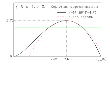
fig:crz-y

3.3 $\xi{\,{\propto}\,}R$ and $n{\,{=}\,}\gamma(R_{E}){\,{-}\,}1$

The approximation that results from our recipe for this choice of $\xi$ and $n$, giving

$$x=(R/R_{E})^{2/\gamma},$$ (48)

is of particular interest. For the harmonic and Kepler potential, this yields, respectively, Kalnajs’ epicycle theory and the Keplerian approximation, i.e. the exact solutions. For other potentials, $n$ is non-integer, and consequently $t(\eta)$ is not analytical. However, one may still give $R$ and $p_{R}$ as functions of $\eta$ and evaluate $J_{R}$. Here are the basic results (with $\delta_{x}{\,{=}\,}x{\,{-}\,}1$ and $L_{c}{\,{=}\,}L_{c}(R_{E})$)

$$Y = L_{c}^{2}\left[e^{2}{\,{-}\,}\delta_{x}^{2}{\,{-}\,}\left(\gamma{-}1{+}\case{\gamma}{3}\case{{\rm d}\ln\kappa^{2}}{{\rm d}\ln R^{2}}\right)\delta_{x}^{3}{\,{+}\,}{\cal O}(\delta_{x}^{4})\right],$$ (49)

$$e = \sqrt{1-L^{2}/L_{c}^{2}},$$ (50)

$$R = R_{E}\,\big{(}1-e\cos\eta\big{)}^{\gamma/2},$$ (51)

$$\kappa t = {\textstyle\int}_{0}^{\eta}\big{(}1-e\cos\eta^{\prime}\big{)}^{\gamma-1}\,{\rm d}\eta^{\prime},$$ (52)

$$J_{R} = \case{\gamma}{2}(L_{c}-|L|).$$ (53)

Note that the neglected third-order term in (49) is usually small: in the case of power-law rotation curves, $v_{c}{\,{\propto}\,}R^{\beta}$, its coefficient becomes maximal in magnitude (at $-0.0572\dots$) for $\beta{\,{=}\,}0$. For this worst case of a flat rotation curve, Figure 5 plots $Y(x)$ and its quadratic approximation. Evidently, this approximation is superb, even for small angular momenta. In particular, it always gives a peri-center radius of zero for $L{\,{=}\,}0$, which all the other approximations fail to do (apart from the cases where they are exact). Note that the radial frequency

$$\omega_{R}=\kappa\,\left[\big{(}|L|/L_{c}\big{)}^{\gamma-1}\,P_{\gamma-1}\big{(}L_{c}/|L|\big{)}\right]^{-1},$$ (54)

where $P_{\nu}(x)$ denotes the associated Legendre function, is larger than $\kappa$, unless $L{\,{=}\,}L_{c}$, $\gamma{\,{=}\,}1$, or $\gamma{\,{=}\,}2$.

Integrating $\dot{\phi}{\,{=}\,}\partial\hat{H}/\partial L$ gives

$$\phi = \theta_{\phi}+\gamma\left[{\eta-\theta_{\!R}\over 2}+A\left(\sqrt{1+e\over 1-e},{\eta\over 2}\right)\right],$$ (55)

$$\omega_{\phi} = \Omega\,{\omega_{R}\over\kappa}+{\partial g\over\partial L},$$ (56)

$$g = \int_{E_{c}(R_{L})}^{E}\!\!\!{\rm d}E\left({\omega_{R}\over\kappa}\left[1-\gamma^{2}{\textstyle{{\rm d}\ln\gamma\over{\rm d}\ln R^{2}}}\Big{(}1{\,{-}\,}{\textstyle{|L|\over L_{c}}}\Big{)}\right]{\,{-}\,}1\right).$$ (57)

with $\theta_{\phi}{\,{=}\,}\omega_{\phi}t$ and $\theta_{\!R}{\,{=}\,}\omega_{R}t$. For a flat rotation curve,

$${\partial g\over\partial L}=-{\Omega\over\sqrt{1-e^{2}}}\left[{\omega_{R}\over\kappa}-1\right].$$ (58)

Figure 5: The approximation arising from $\xi{\,{\propto}\,}R$ and $n{\,{=}\,}\gamma{\,{-}\,}1$ for the logarithmic potential. The solid line gives $Y(x)$ (11), while its quadratic approximation (49) is shown as broken line. The thin horizontal line corresponds to an orbit with $L{\,{=}\,}0.9L_{c}(E)$.

Figure 6: The approximations described in §4 for the logarithmic potential. The solid line gives $Y(x)$ (11), while the dashed and dotted lines correspond to the approximation (59) for $k_{\rm max}{\,{=}\,}1$ and $k_{\rm max}{\,{=}\,}2$, respectively, for the two orbits with $L/L_{c}(E){\,{=}\,}0.4$ and 0.9 (for the latter the approximations can hardly be distinguished from the exact relation).

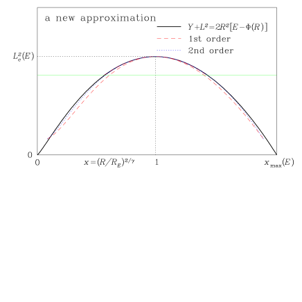
fig:new-y

4 A NEW ORBIT APPROXIMATION

The remarkably accurate orbit approximation presented in §3.3 above has the unfortunate drawback, that the time $t$ cannot explicitly solved for, because the integral in equation (52) is generally not analytically soluble. However, one may approximately solve this integral, by replacing its integrand by a finite powers series in $e$. If the highest power retained in this procedure is $e^{k_{\rm max}}$, this technique amounts to approximating, in the formalism of §2,

$$Y=R^{2}p_{R}^{2}\approx L_{c}^{2}\,(e^{2}-\delta_{x}^{2})\;\left[{x^{\gamma-1}\over\sum_{k=0}^{k_{\rm max}}{\gamma-1\choose k}\delta_{x}^{k}}\right]^{2}.$$ (59)

For the case of a flat rotation curve, Figure 6 plots $Y(x)$ and the approximation (59) with $k_{\rm max}{\,{=}\,}1$ (dashed) and $k_{\rm max}{\,{=}\,}2$ (dotted) for the two orbits with $L/L_{c}{\,{=}\,}0.4$ and 0.9. Evidently, these approximations are not much worse than their parent, i.e. equation (49), and at least as good as the isochrone approximation above. The radial motion, $R(t)$, is given by

$$R = R_{E}\,\big{(}1-e\cos\eta\big{)}^{\gamma/2},$$ (60)

$$e = \sqrt{1-L^{2}/L_{c}^{2}},$$ (61)

$$\kappa t = \eta-e\,(\gamma{-}1)\sin\eta$$ (62)

$$+\case{1}{4}e^{2}(\gamma{\,{-}\,}1)(\gamma{\,{-}\,}2)(\eta+\case{1}{2}\sin 2\eta)+\dots,$$

$$\omega_{R} = \kappa\,\left[1+\case{1}{4}e^{2}(\gamma{\,{-}\,}1)(\gamma{\,{-}\,}2)+\dots\right]^{-1}.$$ (63)

Equation (63) implies $\omega_{R}{\,{\geq}\,}\kappa$ since always $1{\,{\leq}\,}\gamma{\,{\leq}\,}2$, and is, for power-law rotation curves, even more accurate than its parent (54), i.e. including terms ${\cal O}(e^{4})$ would degrade the accuracy of the new approximation. Note that the corresponding radial action cannot be given in closed form. The azimuthal motion may be approximated using equation (55) and replacing $\partial g/\partial L$ by its result for a flat rotation curve (which for power-law models makes an error of the order $e^{4}$):

$$\phi = \omega_{\phi}t+\gamma\left[{\eta-\omega_{R}t\over 2}+A\left(\sqrt{1+e\over 1-e},{\eta\over 2}\right)\right],$$ (64)

$$\omega_{\phi} = \Omega\left[{\omega_{R}\over\kappa}-{1\over\sqrt{1-e^{2}}}\Big{(}{\omega_{R}\over\kappa}-1\Big{)}\right].$$ (65)

The relation (62) for $t(\eta)$ is generally not invertible. As a consequence, one must either (i) use $\eta$ rather than $t$ as independent variable, (ii) solve (62) numerically for $\eta(t)$, or (iii) use the approximate inversion

$$\eta \approx \omega_{R}t+e(\gamma{\,{-}\,}1)\sin\omega_{R}t$$ (66)

$$+\case{1}{8}e^{2}(\gamma{\,{-}\,}1)(3\gamma{\,{-}\,}2)\sin 2\omega_{R}t.$$

Note, however, that using this relation is not equivalent to using (62), rather it generates a different orbit approximation.

As we will see below, the orbit approximation defined by equations (4) is remarkably accurate down to high eccentricities. However, it is not Hamiltonian, i.e. the phase-space flow generated is in general not incompressible. It deviates from this ideal by an amount of the order $e^{k_{\rm max}+1}$.

Figure 7: Surfaces of the $R$-$p_{R}$ section of phase space: comparison of exact orbits in the logarithmic potential, which supports a flat rotation curve, with the predictions of the various orbit approximation of §3 and §4. The orbital angular momenta are, from inside out, 0.98, 0.95, 0.9, 0.85, 0.8, 0.7, 0.6, and 0.5 of $L_{c}(E)$.

Figure 8: Surfaces of the $R$-$(\phi{\,{-}\,}\omega_{\phi}t)$ section of phase space: comparison of exact orbits in the logarithmic potential, which supports a flat rotation curve, with the approximations for the azimuthal motion. The orbits have the same angular momenta as in Figure 7. Approximations which allow for a canonical map to a set of action-angle variables are indicated as ‘AAV’. Note that multiplying the $y$-axis with $R$, these essentially are the epicycles which the orbits perform around their guiding centers.

5 COMPARISON WITH EXACT ORBITS

We now compare the various orbit approximations with numerically integrated orbits in the logarithmic potential, $\Phi{\,{=}\,}v_{0}^{2}\ln(R/R_{0})$, which supports a flat rotation curve. This potential is scale invariant, i.e. all orbits with the same ratio $|L|/L_{c}(E)$ but different energies are identical, apart from a scaling relation or the sense of rotation.

fig:RpR

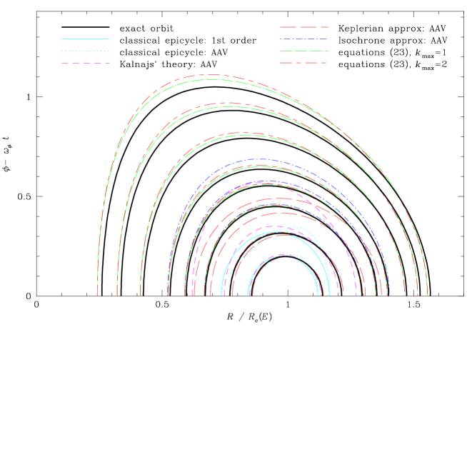
5.1 Testing the Radial Motion

For eight orbits with $|L|/L_{c}(E)$ between 0.5 and 1, Figure 7 compares the plots of $R$ vs. $p_{R}$ (surfaces of section) predicted from the various orbit approximations with the exact relations. The agreement in this plot is indicative of the accuracy of the relation for $R(t)$. For a quantitative comparison with the orbit of a star with velocity $(U,V,W)$ in the solar neighborhood, one should compare $p_{R}$ with the radial velocity $U$. The azimuthal velocity $V$ w.r.t. the local standard of rest can be evaluated from the ratios $R/R_{c}(E)$ and $L/L_{c}(E)$ to be $V{\,{=}\,}\big{(}[L/L_{c}(E)]/[R/R_{c}(E)]-1\big{)}v_{0}$ with $v_{0}$ denoting the local circular speed.

Evidently, Lindblad’s classical epicycle theory becomes significantly inaccurate for $|L|{\,{\la}\,}0.98L_{c}$, corresponding in the solar neighborhood to stars with $|U|\ga 45$$\,{\rm km}\,{\rm s}^{-1}$ or $|V|\ga 32$ ${\rm km}\,{\rm s}^{-1}$ (with $v_{0}{\,{\approx}\,}220\mbox{$\,{\rm km}\,{\rm s}^{-1}$}$). A significant fraction of old-disk stars in the solar neighborhood have velocities in excess of these values (cf. Dehnen, 1998), i.e. the classical epicycle theory cannot be safely used in quantitative studies of the local Galactic disk.

Kalnajs’ epicycle theory is applicable down to $|L|\approx 0.95L_{c}(E)$. Theories with $n{\,{=}\,}1$ are better than the epicycle theories ($n{\,{=}\,}0$). The Keplerian approximation predicts too large peri-centers for $|L|{\,{\la}\,}0.85L_{c}(E)$, and is thus just capable of describing $R(t)$ for stars in the high-velocity tail of the local stellar disk distribution. The isochrone approximation is superior to these, giving accurate approximations down to $|L|{\,{\approx}\,}0.7L_{c}(E)$.

Also shown are the relations arising from the approximations in §3.3 and §4. Evidently, these are very good: the approximation derived in §3.3 and its second-order expansion (equations 4 with $k_{\rm max}{\,{=}\,}2$) are much better than any of the other approximations. Even the first-order expansion ($k_{\rm max}{\,{=}\,}1$) is comparable in accuracy to the isochrone approximation, which itself is second-order accurate.

Figure 9: Radial action $J_{R}$ (left column) and frequency $\omega_{R}$ (middle column) and azimuthal frequency $\omega_{\phi}$ (right column): comparison with exact orbits for the potentials supporting the rotation curves $v_{c}{\,{\propto}\,}R^{\beta}$ with $\beta{\,{=}\,}{-}0.2$, 0, and 0.2 (from top to bottom). Note that $\omega_{R}{\,{=}\,}\kappa(E)$ for all these approximations except Lindblad’s epicycle theory and the approximation of §4 with $k_{\rm max}{\,{=}\,}2$ (equation 63, second order).

fig:Rphi

5.2 Testing the Azimuthal Motion

To test the quality of the approximations for the azimuthal motion, I compare in Figure 8 the surfaces of $R$-($\phi{\,{-}\,}\omega_{\phi}t)$ sections of the same orbits as in Figure 7 with some of the approximtions.

The approximations for which $\phi(t)$ has been obtained such as to yield a canonical map to a set of action-angle variables, are indicated as ‘AAV’ in the figure index. Among these approximation, the order of accuracy is similar as for the radial motion, but they are less accurate in this section of phase space than in the $R$-$p_{R}$ section. This is not surprising, as the approximations were designed to approximate $R(t)$, and any deviation from the true $R(t)$ is likely to be amplified when integrating for $\phi(t)$.

Figure 8 also plots three orbit approximations which do not yield a canonical map to action-angle variables: the textbook variant of the classical epicycle theory and the new approximation of §4 for first- and second-order expansions. This variant of the epicycle theory is clearly superior in accuracy to its canonical counterpart, i.e. enforcing a canonical mapping degrades the accuracy of the approximation. The two approximations resulting from equations (4) are much more accurate than all the others, though they are slightly less accurate than in the $R$-$p_{R}$ surface of section. Strangly, the first-order approximation is more accurate than the second-order.

fig:joo

5.3 Testing Frequencies and the Radial Action

In Figure 9, the radial action and orbital frequencies predicted by the orbit approximations are compared with the exact ones for all orbits in the potentials supporting nearly flat rotation curves $v_{c}{\,{\propto}\,}R^{\beta}$ with $\beta{\,{=}\,}{-}0.2$, 0, and 0.2. Even for nearly eccentric orbits, the classical epicycle approximation under-estimates $J_{R}$ and drastically over-estimates the frequencies. The three approximations with $\xi{\,{\propto}\,}R$ and integer $n$ (Kalnajs, Keplerian, isochrone) have $\omega_{R}{\,{=}\,}\kappa(R_{E})$, which actually is not a bad description of the truth. Similarly, $\omega_{\phi}{\,{=}\,}\Omega(R_{E})$ is a reasonably good estimate. The estimates for $\omega_{R}$ from the orbit approximations with canonical maps to action-angle variables are only useful for large $L$, corresponding to small $e$.

I also plotted the estimates (63) and (65) for $\omega_{R}$ and $\omega_{\phi}$ respectively. While the latter becomes inaccurate at $L{\,{\la}\,}0.5L_{c}$, the estimate for $\omega_{R}$ is very accurate for all $L$ (the corresponding lines are almost entirely overlaid by those for the exact relations).

At $L{\,{\approx}\,}L_{c}(E)$, all orbit approximations give $J_{R}$ correctly, insomuch that they agree in the linear term when expanding $J_{R}$ as power series in $1{\,{-}\,}|L|/L_{c}$. This linear relation is actually the result for $J_{R}$ obtained from the approximation of §3.3.

6 CONCLUSIONS

The classical epicycle theory of Lindblad (1926) is usually derived starting from the Hamiltonian or, equivalently, from the equations of motions for a near-circular orbit in a spherical or flat axisymmetric potential. In this paper, I instead directly considered the integral (1) to be solved in order to obtain $R(t)$. The simplest way to approximate this integral by some closed form leads straight to the classical epicycle theory. In Section 2, I derive a general method for approximating this integral in a better way by manipulating the integrand before approximating it.

6.1 Relation to Other Work

Several published studies deal with improved approximations for the stellar orbits. Most of them start with Lindblad’s classical epicycle theory and try to improve it by extension to higher orders, variations of the constants involved, or both. Apart from the quoted paper of Kalnajs, I know of only one more study, Shu (1969), in which an orbit approximation is derived that does not incorporate Lindblad’s theory.

Shu also considers directly the integral (1) and manipulates it to obtain approximate solutions. Unlike this work, Shu uses a (truncated) power-series expansion in the eccentricity, the lowest order of which yields Lindblad’s theory, while the next order yields an approximation that becomes exact in the case of Keplerian motion. This approximation is not quite the same, though, as the Keplerian approximation above, for example, the radial frequency for Shu’s theory is $\omega_{R}{\,{=}\,}(1{\,{-}\,}e^{2})^{3/2}\kappa(R_{L})$ with $e$ given in equation (23), while the approximation proposed in Section 3.2.2 has $\omega_{R}{\,{=}\,}\kappa(R_{E})$.

6.2 New Orbit Approximations

From the general recipe in Section 2, endlessly many orbit approximations may be derived. In Section 3, four of them are presented in addition to the classical epicycle theory. One has already been introduced by Kalnajs (1979) and becomes exact for the harmonic potential. Two other approximation yield the exact orbits for the potentials of, respectively, a central point mass and Hénon’s (1959) isochrone sphere, and I call them accordingly Keplerian and isochrone approximations. A comparison with exact orbits in the logarithmic potential, which supports a flat rotation curve, shows that the latter two approximations are better than Kalnajs’, which in turn is superior to the classical epicycle theory. In particular, they may safely be applied even to the high-velocity tail of the stellar old-disk population.

The fourth new orbit approximation may be considered a hybrid between Kalnajs’ theory and the Keplerian approximation, it is very accurate, even for purely radial orbits, for potentials with power-law rotation curves, $v_{c}{\,{\propto}\,}R^{\beta}$. However, this approximation has the severe drawback that the time cannot explicitly be solved for.

6.3 Action-Angle Variables

After obtaining an approximation for $R(t)$, I also consider the task of integrating the azimuthal motion such that the resulting approximation for the phase-space flow is incompressible, as Liouville’s theorem demands. This is equivalent to obtaining an approximate but canonical map to a set of action-angle variables $(J_{R},L,\theta_{\!R},\theta_{\phi})$. For Lindblad’s and Kalnajs’ epicycle theories, as well as for the new Keplerian and isochrone approximation, this map can be given explicitly. However, the azimuthal frequency $\omega_{\phi}$ that is consistent with this map cannot be expressed in closed form, except for the classical epicycle theory or otherwise for special potentials (the logarithmic potential and that for which the respective approximation is exact).

Using an approximation for the azimuthal motion that does not yield an incompressible phase-space flow may lead to spurious effects. An example for such an approximation is the textbood variant of Lindblad’s classical epicycle theory. In Section 3.1.1, a version of this theory is presented that does not suffer from this problem.

6.4 Estimates of Orbital Properties

In face of the ease by which stellar orbits can be computed numerically, orbit approximations may be most important as a tool for quantitative estimates of stellar dynamical processes, in particular in dynamically cool stellar disks. However, a comparison of the approximations with integrated orbits in Section 5 showed that the classical epicycle theory greatly over-estimates the orbital frequencies and under-estimates the peri- and apo-center and radial action. Consequently, quantitative analyses based on this approximation will inevitably involve systematic errors. The size of these error may reach 10% of more already for slightly eccentric orbits, which in the solar neighborhood correspond to velocities w.r.t. LSR in excess of about 40$\,{\rm km}\,{\rm s}^{-1}$.

Highly accurate estimates for the orbital quantities may be derived from the orbit approximation presented in Section 3.3. This approximation, even though it does not yield $R(t)$ in closed form, is very accurate for orbits in potentials which support nearly flat rotation curves, like that of the Galaxy. The resulting estimates for the peri- and apo-centers are

$$R_{\pm}(E,L)\approx R_{c}(E)\,(1\pm e)^{\gamma(E)/2}$$ (67)

with eccentricity

$$e^{2}=1-L^{2}/L_{c}^{2}(E)$$ (68)

and $\gamma{\,{\equiv}\,}2\Omega/\kappa$. Here, $R_{c}(E)$, $L_{c}(E)$, $\Omega(E)$, and $\kappa(E)$ denote the radius, angular momentum, azithmal frequency, and epicyclic frequency, respectively, of the circular orbit with the same energy $E$ as the orbit in question. For orbits in potentials with power-law rotation curves $v_{c}{\,{\propto}\,}R^{\beta}$, equation (67) under-estimates the apo-center by at most 1.7% (for $L{\,{=}\,}0$, $\beta{\,{\approx}\,}{-}0.16$), while the peri-center is under-estimated by at most ${\,{\sim}\,}2\%$ (for $L{\,{\approx}\,}0.3L_{c}$, $\beta{\,{\approx}\,}0.1$). The corresponding estimate for the radial action is

$$J_{R}(E,L)\approx\case{1}{2}\,\gamma(E)\,\big{(}L_{c}(E)-|L|\big{)}.$$ (69)

For power-law rotation curves, the largest error of this estimate occurs on purely radial orbits ($L{\,{=}\,}0$) in the logarithmic potential ($\beta{\,{=}\,}0$), where actually $J_{R}{\,{=}\,}L_{c}\sqrt{{\rm e}/2\pi}$ on radial orbits (equation 84), while the above approximation predicts a value 7.5% larger.

Another way to use this very accurate orbit approximation is to further approximate it, in order to overcome its major drawback and solve for the time explicitly. This results in a new orbit approximation, presented in Section 4, which gives $R(t)$ and is still very accurate to high eccentricities. The corresponding approximation for the radial frequency

$$\omega_{R}(E,L)\approx\kappa(E)/\big{(}1+\case{e^{2}}{4}(\gamma-1)(\gamma-2)\big{)}$$ (70)

is, for power-law rotation curves, accurate to better than 1.4% (at $L{\,{=}\,}0$, $\beta{\,{\approx}\,}0.3$), while the rough estimate $\omega_{R}(E,L)\approx\kappa(E)$ under-estimates the radial frequency by at most 7.5% (at $L{\,{=}\,}0{\,{=}\,}\beta$). The azimuthal frequency, which may be expressed as the time average of $LR^{-2}$, is the orbital quantity most difficult to estimate, because it is very sensitive to $R(t)$ near peri-center, where the approximations for the radial motion are least accurate. Numerical experiments suggest that the simple estimate

$$\omega_{\phi}\approx\Omega(E)$$ (71)

is still the most useful: it becomes inaccurate at the ${\ga}10\%$ level for orbits with $L{\,{\la}\,}0.3L_{c}$.

Equations (67) to (71) provide accurate and yet simple estimates for basic orbital properties in typical galactic potentials. Note however, that these estimates are not self-consistent, i.e. they do not in general satisfy $\omega_{R}{\,{=}\,}(\partial E/\partial J_{R})_{L}$ or $\omega_{\phi}{\,{=}\,}(\partial E/\partial L)_{J_{R}}$.

Appendix A CIRCULAR ORBITS

This appendix summarizes the relations between the quantities describing circular orbits. While some of these relations are well-known, several others, even though trivial in principle, are less familiar. A circular orbit at radius $R$ is defined by equilibrium between gravitation and centrifugal forces, resulting in the relation

$$v_{c}^{2}(R){\,{=}\,}R^{-1}(\partial\Phi/\partial R)$$ (72)

for its azimuthal velocity. A circular orbit is uniquely determined by either its radius $R$, angular momentum $L$, energy $E$, circular frequency $\Omega$, or radial frequency $\kappa$, also known as epicycle frequency. (Radial oscillations are not excited for circular orbits, but their radial frequency is well-defined nonetheless). The definitions and some relations between these are

$$L_{c}^{2} \equiv R^{2}\,v_{c}^{2}=R^{3}{\partial\,\Phi\over\partial R}=R^{4}\,\Omega^{2};$$ (73)

$$E_{c} \equiv {v_{c}^{2}\over 2}+\Phi={\partial(R^{2}\,\Phi)\over\partial R^{2}};$$ (74)

$$\Omega^{2} \equiv R^{-2}\,v_{c}^{2}=R^{-4}\,L_{c}^{2}=R^{-1}{\partial\,\Phi\over\partial R}=\left({{\rm d}E_{c}\over{\rm d}L_{c}}\right)^{2};$$ (75)

$$\kappa^{2} \equiv \left({\partial^{2}\over\partial R^{2}}\!\Big{[}\Phi{\,{+}\,}{L^{2}\over 2R^{2}}\Big{]}\right)_{\!L=L_{c}}={\partial^{2}\Phi\over\partial R^{2}}+{3\over R}{\partial\,\Phi\over\partial R}$$ (76)

$$= {1\over R^{3}}{{\rm d}L^{2}_{c}\over{\rm d}R}=R{{\rm d}\,\Omega^{2}\over{\rm d}R}+4\,\Omega^{2}$$ (77)

$$= 4{{\rm d}E_{c}\over{\rm d}R^{2}}=4{\partial^{2}(R^{2}\,\Phi)\over\partial(R^{2})^{2}};$$ (78)

$${{\rm d}\Omega\over{\rm d}E} = {1-\gamma^{2}\over L_{c}},$$ (79)

where

$$\gamma\equiv{2\Omega\over\kappa}.$$ (80)

Appendix B POWER-LAW POTENTIALS

Quite often one is dealing with simple power-law models with circular speed

$$v_{c}(R)=v_{0}\left({R\over R_{0}}\right)^{\beta}$$ (81)

and gravitational potential

$$\Phi(R)=v_{0}^{2}\times\left\{\begin{array}[]{l@{$\quad$}l}\displaystyle{1\over 2\beta}\left(R\over R_{0}\right)^{2\beta}&{\rm for\;}\beta\neq 0\\[8.61108pt] \displaystyle\ln\left(R\over R_{0}\right)&{\rm for\;}\beta=0.\end{array}\right.$$ (82)

Here, $R_{0}$ and $v_{0}$ are scale radius and scale velocity, and shall be set to unity in the remainder of this Appendix. The power-law index is restricted to $\beta\,{\in}\,[{-}\case{1}{2},\,1]$ with $\beta{\,{=}\,}1$ and ${-}\case{1}{2}$ corresponding to, respectively, the harmonic potential and that created by a point mass at the origin. The fundamental quantities of circular orbits expressed as functions of radius, angular momentum, or energy are listed in Table 1, while the relations for $\kappa$ follow from

$$\gamma=\sqrt{2/(1+\beta)}.$$ (83)

Table 1: Relations for circular orbits in power-law potentials (82) in units that imply $R_{0}{\,{\equiv}\,}1{\,{\equiv}\,}v_{0}$.

quantity	expressed as function of
	$R$	$L$	$E,\,\beta{\,{\neq}\,}0$	$E,\,\beta{\,{=}\,}0$
$v$	$R^{\beta}$	$L^{\beta\over 1+\beta}$	$\left({2\beta\over 1+\beta}E\right)^{1\over 2}$	1
$R$	$R$	$L^{1\over 1+\beta}$	$\left({2\beta\over 1+\beta}E\right)^{1\over 2\beta}$	${\rm e}^{E-1/2}$
$L$	$R^{1+\beta}$	$L$	$\left({2\beta\over 1+\beta}E\right)^{1+\beta\over 2\beta}$	${\rm e}^{E-1/2}$
$E,\,\beta\,{\neq}\,0$	${1+\beta\over 2\beta}R^{2\beta}$	${1+\beta\over 2\beta}L^{2\beta\over 1+\beta}$	$E$
$E,\,\beta{\,{=}\,}0$	$\case{1}{2}+\ln R$	$\case{1}{2}+\ln L$		$E$
$\Omega$	$R^{\beta-1}$	$L^{\beta-1\over\beta+1}$	$\left({2\beta\over 1+\beta}E\right)^{\beta-1\over 2\beta}$	${\rm e}^{1/2-E}$

In general, the radial action $J_{R}$ cannot be expressed in terms of elementary functions of $(E,L)$; however, for the purely radial orbits with $L{\,{=}\,}0$, $J_{R}$ may be given in closed form:

$${J_{R}(L{=}0)\over L_{c}(E)}=\left\{\begin{array}[]{l@{$\quad$}l}\displaystyle{(1+\beta)^{1+\beta\over 2\beta}\,\Gamma\left({1+\beta\over-2\beta}\right)\over\sqrt{2\pi}\,|2\beta|^{3/2}\,\Gamma\left({1-2\beta\over-2\beta}\right)}&{\rm for}\;\beta<0,\\ \displaystyle\sqrt{{\rm e}\over 2\pi}&{\rm for}\;\beta=0,\\ \displaystyle{(1+\beta)^{1+\beta\over 2\beta}\,\Gamma\left({1\over 2\beta}\right)\over\sqrt{2\pi}\,(2\beta)^{3/2}\,\Gamma\left({1+3\beta\over 2\beta}\right)}&{\rm for}\;\beta>0.\end{array}\right.$$ (84)

Appendix C THE ISOCHRONE APPROXIMATION

The approximation for $R(t)$ and $\phi(t)$ resulting from the the isochrone approximation of §3.2.1 are

$$R^{2}(t) = (R_{E}^{2}+b^{2})\,\big{(}1-e\cos\eta\big{)}^{2}-b^{2},$$ (85)

$$\theta_{\!R} = \kappa t=\eta-e\,\sin\eta,$$ (86)

$$e = \sqrt{\Delta L^{2}}\big{/}\big{(}x_{0}^{2}\,\kappa\big{)}=\case{\gamma}{2}(1{\,{-}\,}b^{\prime 2})\sqrt{1-L^{2}/L_{c}^{2}},$$ (87)

$$J_{R} = x_{0}^{2}\,\kappa\bigg{[}1-\case{1}{2}\sum_{\pm}\sqrt{(1\pm b^{\prime})^{2}{\,{-}\,}e^{2}}\,\bigg{]};$$ (88)

$$\phi(t) = \theta_{\phi}+{e\,\hat{\omega}_{\phi}\over\kappa}\sin\eta+{L\over x_{0}^{2}\kappa}\sum_{\pm}{A\!\left(\!\sqrt{1{\,{+}\,}e{\,{\pm}\,}b^{\prime}\over 1{\,{-}\,}e{\,{\pm}\,}b^{\prime}},{\eta\over 2}\!\right)\over\sqrt{(1\pm b^{\prime})^{2}{\,{-}\,}e^{2}}},$$ (89)

$$\theta_{\phi} = \omega_{\phi}t,$$ (90)

$$\omega_{\phi} = \hat{\omega}_{\phi}+{\partial g\over\partial L},$$ (91)

$$\hat{\omega}_{\phi} = {L\over 2x_{0}^{2}}\sum_{\pm}{1\over\sqrt{(1\pm b^{\prime})^{2}{\,{-}\,}e^{2}}},$$ (92)

$$g = \int_{E_{c}(R_{L})}^{E}\!\!\!\!\!\!{\rm d}E\;\kappa^{2}{{\rm d}b^{2}\over{\rm d}E}\left[1{\,{-}\,}{1\over 4b^{\prime}}\sum_{\pm}{\pm(1{\,{\pm}\,}b^{\prime})^{3}\over\sqrt{(1{\pm}b^{\prime})^{2}{-}e^{2}}}\right]\!$$ (93)

with $b^{\prime}{\,{\equiv}\,}b/x_{0}$. Here, I have assumed that $b$ was chosen according to (38), which gives ${\rm d}\kappa/{\rm d}E{\,{=}\,}{-}3\kappa^{-1}x_{0}^{-2}$ and

$$L\,x_{0}^{-2} = \Omega(R_{E})\sqrt{(1-b^{\prime 2}-2e^{2}\gamma^{-2})(1-b^{\prime 2})}$$ (94)

$$\kappa^{2}{{\rm d}b^{2}\over{\rm d}E} = -10+{8x_{0}^{4}\over 3\kappa^{2}}\left[{{\rm d}^{2}\kappa^{2}\over{\rm d}(R^{2})^{2}}\right]_{R_{E}}.$$ (95)

For the isochrone potential (39), $g{\,{=}\,}0$, while for a flat rotation curve,

$${\partial g\over\partial L}=-{2v_{0}^{2}\over L}\left[1{\,{-}\,}{1\over 4b^{\prime}}\sum_{\pm}{\pm(1\pm b^{\prime})^{3}\over\sqrt{(1{\pm}b^{\prime})^{2}{-}e^{2}}}\right].$$ (96)

References

- [Binney & Tremaine 1987] Binney J.J., Tremaine S., 1987, Galactic Dynamics. Princeton Univ. Press, Princeton
- [Dehnen 1998] Dehnen W., 1998, AJ, 115, 2384
- [Hénon 1959] Hénon M., 1959, Ann. Astrophys. 22, 126
- [Kalnajs 1979] Kalnajs A.J., 1979, AJ, 84, 1697
- [Lindblad 1926] Lindblad B., 1926, Arkiv f. Matematik, Astronomi och Fysik 19A, 27 (see also Uppsala Medd. 4)
- [Lindblad 1958] Lindblad B., 1958, Stockholms Obs. Ann., 20, 4
- [Shu 1969] Shu F.H., 1969, ApJ, 158, 505