Simple Distribution Functions for Stellar Disks

Abstract

Distribution functions (DFs) for dynamically warm thin stellar disks residing in arbitrary axisymmetric potentials are presented which approximately reproduce pre-described surface-density and velocity-dispersion profiles. The functional form of the DFs is obtained by ‘warming-up’ a model made entirely of circular orbits. This can be done in various ways giving different functional forms for the DF. In the best case, the DF reproduces the pre-described profiles to within a few per cent for a typical case reminiscent to the old stellar disk in the Milky Way. This match may be improved to about one per cent or better by a simple iterative method. An algorithm is given to draw phase-space points randomly from the DFs for the purpose of, e.g., $N$-body simulations. All the relevant computer programs are available from the author.

scheduled for publication in the September 1999 issue of The Astronomical Journal

1 INTRODUCTION

All the dynamical properties of a collisionless stellar system are prescribed by its phase-space distribution function (DF) in conjunction with the underlying gravitational potential $\Phi$. The knowledge of a simple DF is often vital for studies of the dynamical state of stellar systems, their equilibrium properties and time-evolution. In this paper, simple DFs for thin axisymmetric disks are given. These DFs may be used in studies of, e.g., spiral structure, the effects of non-axisymmetric perturbation on the velocity distribution in the solar neighborhood, and to seed initial conditions for $N$-body simulations.

For a thin axisymmetric disk, $\Phi{\,{=}\,}\Phi(R)$ and the collisionless Boltzmann equation tells us that in dynamical equilibrium the stellar DF must be a function of the stellar energy and angular momentum alone, $f{\,{=}\,}f(E,L)$. Thus, compared to the more general case of three-dimensional axisymmetric or non-axisymmetric systems, where the DF may also depend on non-classical integrals of motion, the DFs of thin axisymmetric disks are simple and allow for mathematical manipulations. It is possible to give a DF $f(E,L)$ which implements some pre-defined properties, for example, a certain surface density profile $\Sigma(R)$, in a given underlying gravitational potential $\Phi(R)$. Unfortunately however, this DF is highly non-unique: every one of the infinitely many ways to expand $\Sigma(R)$ as a function of both $R$ and $\Phi(R)$, and thus to obtain a so-called surface-density partition $\Sigma(R,\Phi)$, determines uniquely the part of the DF even in $L$ ([Kalnajs 1976]). This even part of the DF, $f_{+}$, can be computed (usually numerically) by a path-integral ([Hunter & Qian 1993]). Additional constraints, for example, a certain radial-velocity-dispersion profile $\sigma_{R}(R)$, restrict the possible surface-density partitions and thus DFs, but do not remove the general degeneracy (obviously, the DF being a function of two variables cannot be uniquely determined by a finite set of functions of one variable).

Given this degeneracy among possible disk DFs, there are two different ways to construct specific dynamical models. The first approach follows the above lines in specifying a particular surface-density partition and then solving for the implied $f_{+}(E,L)$. This technique has the advantage that the pre-defined properties are exactly satisfied by the resulting DF, but the disadvantage that the DF can rarely be given in closed form, which tends to be complicated.

The second way to a disk DF is to specify a particular functional form, that results only in approximate agreement with the pre-defined properties. This approach has the advantage that the DF is always of a simple functional form, which often is of great importance in dynamical modeling. Another bonus is that the degeneracy among DFs with given surface density and velocity dispersion is removed by choosing a particular functional form for the DF itself rather than the partition function. This enables one to choose the functional form for $f(E,L)$ on the basis of astro-physical arguments. On the other hand, in the first approach the degeneracy is often exploited by choosing the surface-density partition such that the resulting DF is analytic.

The aim of this paper is to improve and extend on what has been done before on that second approach to warm-disk DFs. In Section 2, warm-disk DFs are constructed by warming-up the DF for a completely cold disk in which all stars on circular orbits. In Section 3, the ability of four types of warm-disk DFs to reproduce the predefined surface-density and velocity-dispersion profile is assessed and a simple algorithm is given to improve on this ability. Section 4 compares the velocity moments up to fourth-order for the four DFs introduced in Section 2, while Section 5 gives an algorithm for drawing from the DFs samples of phase-space points such as might be used for numerical simulations.

2 RECIPES FOR WARM-DISK DISTRIBUTION FUNCTIONS

We seek DFs $f(E,L)$ which approximately create given targets for the surface density $\Sigma(R)$ and radial velocity dispersion $\sigma_{R}(R)$ in a given potential $\Phi(R)$. The basic technique is to modify the DF for a completely cold disk.

2.1 The Distribution function for the cold disk

Let $E_{c}(L)$ be the energy of the circular orbit with angular momentum $L$ (see, e.g., Appendix A of Dehnen 1999, hereafter paper I, for details of the properties of circular orbits), then

$${f_{\rm cold}}(E,L)={f_{\rm circ}}(L)\;\delta\big{(}E-E_{c}(L)\big{)},$$ (1)

describes a DF which allows for circular orbits only. From

$$M=(2\pi)^{2}\int{\rm d}^{2}\!\mbox{\boldmath$J$}\;f,$$ (2)

which may be derived using ${\rm d}^{2}\!\mbox{\boldmath$x$}\,{\rm d}^{2}\!\mbox{\boldmath$v$}\equiv{\rm d}^{2}\!\mbox{\boldmath$J$}\,{\rm d}^{2}\!\mbox{\boldmath$\theta$}$ with $\mbox{\boldmath$J$}\equiv(J_{R},L)$ denoting the action variables, and $(\partial E/\partial J_{R})_{L}\equiv\omega_{R}$, we have

$$M=(2\pi)^{2}\int{\rm d}E\int{\rm d}L\;f(E,L)\;\omega_{R}^{-1}(E,L),$$ (3)

and thus

$${\rm d}M=(2\pi)^{2}{f_{\rm circ}}(L)/\kappa(L)\;{\rm d}L,$$ (4)

where I have used the fact that on circular orbits the radial frequency $\omega_{R}$ equals the epicycle frequency $\kappa$. On the other hand we have

$${\rm d}M=2\pi\,R\;\Sigma(R)\,{\rm d}R,$$ (5)

and equating (4) with (5) gives, with ${\rm d}L_{c}/{\rm d}R{\,{=}\,}R\kappa/\gamma$ (cf. equations A2 to A6 of paper I), ${f_{\rm circ}}(L){\,{=}\,}f_{1}\big{(}R_{c}(L)\big{)}$ with

$$f_{1}(R)\equiv{\gamma(R)\Sigma(R)\over 2\pi}.$$ (6)

Here, $R_{c}(L)$ is the radius of the circular orbit with angular momentum $L$, while $\gamma{\,{\equiv}\,}2\Omega/\kappa$ with the circular frequency $\Omega(R)$.

2.2 The Shu distribution function

In order to allow for non-circular motions, the $\delta$-function in the cold-disk DF (1) must be replaced by some function of finite width. Since the epicycle energy $E-E_{c}(L)$ is non-negative, a simple choice is an exponential corresponding to a Maxwellian velocity distribution

$$\delta\big{(}E-E_{c}(L)\big{)}\;\longrightarrow\;{1\over\sigma_{R}^{2}}\exp\!\left[{E_{c}(L)-E\over\sigma_{R}^{2}}\right].$$ (7)

Using $R_{L}{\,{\equiv}\,}R_{c}(L)$ also as argument of $\sigma_{R}^{2}$, this leads to the well-known DF (Shu 1969)

$${f_{\rm Shu}}(E,L)={\gamma(R_{L})\,\Sigma(R_{L})\over 2\pi\,\sigma_{R}^{2}(R_{L})}\;\exp\!\left[{E_{c}(L){-}E\over\sigma_{R}^{2}(R_{L})}\right].$$ (8)

2.3 New warm-disk distribution functions

Instead of (1), we could have started with the alternative ansatz for a cold-disk DF:

$${f_{\rm cold}}(E,L)={f_{\rm circ}}(E)\;\delta\Big{(}\Omega(E)\big{[}L_{c}(E)-L\big{]}\Big{)}.$$ (9)

With ${\rm d}E_{c}/{\rm d}R{\,{=}\,}R\kappa^{2}/2$, one finds ${f_{\rm circ}}(E)=f_{1}\big{(}R_{c}(E)\big{)}$, where $R_{c}(E)$ is the radius of the circular orbit at energy $E$. As ${f_{\rm Shu}}$ was derived from (1), we may derive a new warm-disk DF from (9):

$${f_{\rm new}}(E,L)={\gamma(R_{E})\,\Sigma(R_{E})\over 2\pi\,\sigma_{R}^{2}(R_{E})}\,\exp\!\left[{\Omega(R_{E})[L{-}L_{c}(E)]\over\sigma_{R}^{2}(R_{E})}\right]$$ (10)

with $R_{E}{\,{\equiv}\,}R_{c}(E)$. There is actually large freedom in designing more warm-disk DFs by combining the various possibilities for the arguments of $f_{1}$, $\sigma_{R}^{2}$, and the exponential. Two other possible DFs are

$${f_{\rm a}}(E,L) = {\gamma(R_{E})\,\Sigma(R_{E})\over 2\pi\,\sigma_{R}^{2}(R_{E})}\;\exp\!\left[{E_{c}(L){-}E\over\sigma_{R}^{2}(R_{E})}\right],$$ (11)

$${f_{\rm b}}(E,L) = {\gamma(R_{L})\,\Sigma(R_{L})\over 2\pi\,\sigma_{R}^{2}(R_{L})}\;\exp\!\left[{\Omega(R_{L})[L{-}L_{c}(E)]\over\sigma_{R}^{2}(R_{L})}\right].$$ (12)

2.4 Physical Motivation

Shu (1969) motivated his DF by the idea that an initial process of violent relaxation formed the distribution function of stellar disks. He also assumed that the initial distribution of angular momenta is not changed by this process. However, we now know, that these ideas are incorrect. Disk stars gain their random motions by scattering off molecular clouds, spiral waves, satellite galaxies and other agents. Therefore, the velocity dispersion grows continuously, which is also reflected in the observed increase of random motions with stellar age in the solar neighborhood. Such scattering processes do not change the value of a star’s Hamiltonian in the frame co-rotating with the scattering agent. This Hamiltonian is equal to the Jacobi energy $E_{J}{\,{=}\,}E{\,{-}\,}\omega L$ with $\omega$ the angular frequency of the scattering agent. Consequently, both the stellar energies and angular momenta are affected by disk heating. Thus, we may describe the DF as a warmed-up version of a DF made from new-born stars. Stars are born already with some finite velocity dispersion, which is small compared to that gained subsequently, and we may safely assume the DF of new-born stars is dynamically completely cold. The warming-up may be described by an exponential in the radial action $J_{R}$ ([Binney 1987])

$$f\approx f_{1}(R_{1})\;{1\over\sigma_{R}^{2}(R_{1})}\,\exp\!\left[-{\omega_{R}J_{R}\over\sigma^{2}_{R}(R_{1})}\right].$$ (13)

Here, $R_{1}{\,{=}\,}R_{1}(E,L)$ is some measure of the mean orbital radius that ensures the prescribed surface density to be closely matched by the DF. The radial action may be estimated from the classical epicycle theory to be

$$\omega_{R}J_{R}\sim E-E_{c}(L),$$

but, as demonstrated in paper I,

$$\omega_{R}J_{R}\approx\Omega(E)\big{[}L_{c}(E)-|L|\big{]}$$

is much better an approximation for near-flat rotation curves. Using either of these approximations for $\omega_{R}J_{R}$ and either $R_{L}$ or $R_{E}$ for $R_{1}$, any of the four DFs presented above can be derived from equation (13).

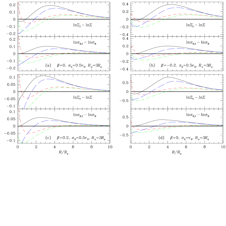
Figure 1: Logarithmic deviations between the target surface density and velocity dispersion ($\Sigma$, $\sigma_{R}$) and those actually created by the warm-disk DF ($\Sigma_{f}$, $\sigma_{R,f}$) in power-law potentials with circular speed $v_{c}{\,{\propto}\,}R^{\beta}$. Solid lines are for ${f_{\rm Shu}}$, dashed for ${f_{\rm new}}$, dot-dash for ${f_{\rm a}}$, and long-dashed for ${f_{\rm b}}$. In all four sub-figures, both $\Sigma$ and $\sigma_{R}$ decay exponentially with scale lengths $R_{\sigma}{\,{=}\,}3R_{s}$. In (a), (b), and (c), the central velocity dispersion is $0.5v_{0}$, while it is twice as large for (d). The rotation curve is flat in (a) and (d), slightly falling in (b) and slightly rising in (c). Notice the different scales of the $y$-axes.

There are two arguments in favor of ${f_{\rm new}}$ being the most useful of these four DFs. First, the mean orbital radius $\overline{R}(E,L)$ is much better approximated by $R_{E}$ than by $R_{L}$ (in general: $R_{L}{\,{\leq}\,}R_{E}{\,{\la}\,}\overline{R}$). Similarly, $\kappa(R_{E})$ approximates the radial frequency $\omega_{R}$, which we replaced by $\kappa$ in the derivation of $f_{1}$, far better than $\kappa(R_{L})$, see, e.g. Fig. 8 of paper I. Therefore, one expects DFs with $R_{1}{\,{=}\,}R_{E}$ to create surface density and velocity dispersion in better agreement with the target functions than DFs with $R_{1}{\,{=}\,}R_{L}$. Second, $\Omega(L{\,{-}\,}L_{c})$ as argument of the exponential naturally extends to negative $L$, while an exponential in $E{\,{-}\,}E_{c}$ does not allow for this possibility. This is significant insofar, as the tail of stars with small negative $L$ is known to be important for supporting disks against dynamical instabilities.

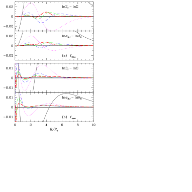
Figure 2: The same as in Fig. 1a, but for the DFs ${f_{\rm Shu}}$ (a) and ${f_{\rm new}}$ (b) after none (thin), one (dotted), two (dashed), three (long-dashed), and four (bold dot-dash) iterations of the scheme of §3.2.1. Notice the different scales on the $y$-axes.

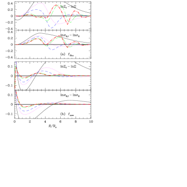
Figure 3: As Fig. 2 but for the stellar disk and rotation curve as in Fig. 1d (which is hot inside $\sim 1.3R_{\Sigma}$) and after none (thin), one (dotted), two (dashed), five (long-dashed), and seven (bold dot-dash) iterations of the scheme of §3.2.1. Notice the different scales on the $y$-axes.

3 ASSESSING THE DISTRIBUTION FUNCTIONS

Allowing for non-circular motions, i.e. replacing the $\delta$-function in (1) or (9) with some function of finite width, leads at any position $R$ to a mixture of stars originating from different radii $R_{1}$. As a consequence, the surface density $\Sigma_{f}(R)$ that is actually created by the DF deviates from the target $\Sigma(R)$. Similarly, the radial velocity dispersion $\sigma_{R,f}(R)$ due to the DF is expected to differ from the target $\sigma_{R}(R)$. On the one hand a simple and generally applicable functional form for the DF is very desirable, on the other hand it is equally important for the DF to re-produce these targets as closely as possible. In §3.1, we assess the ability of the DFs introduced in §2 to satisfy this latter goal, while §3.2 presents a simple numerical method by which the match to the target functions can be vastly improved.

3.1 How Well do the DFs Re-Produce their Targets?

We now specify the target functions $\Sigma(R)$ and $\sigma_{R}(R)$ and compare these with the numerically evaluated velocity moments resulting from the various forms of warm-disk DFs. We restrict ourselves to exponential surface-density and velocity-dispersion profiles

$$\Sigma(R) = \Sigma_{0}\;{\rm e}^{-R/R_{s}}$$ (14)

$$\sigma_{R}(R) = \sigma_{0}\;{\rm e}^{-R/R_{\sigma}}$$ (15)

with scale radii $R_{s}$ and $R_{\sigma}$. The gravitational potential is assumed to be a power-law with circular speed curve $v_{c}{\,{=}\,}v_{0}(R/R_{s})^{\beta}$ (cf. Appendix B of paper I). Furthermore, we only consider models with $R_{\sigma}{\,{=}\,}3R_{s}$ resulting in $\sigma_{R}^{3}{\,{\propto}\,}\Sigma$ corresponding roughly to the situation in the Milky-Way disk. For flat ($\beta{\,{=}\,}0$), slightly rising ($\beta{\,{=}\,}0.2$) or falling ($\beta{\,{=}\,}-0.2$) rotation curves, and for the four warm-disk DFs introduced in the last section, Figure 1 plots the logarithmic deviations of surface density and velocity dispersion for $\sigma_{0}{\,{=}\,}0.5v_{0}$ (Fig. 1a-c), corresponding to $\sigma(R_{0}{\,{\approx}\,}2.5R_{\Sigma}){\,{\approx}\,}0.2v_{0}$ reminiscent of the old-stellar disk of the Milky Way, and doubly as much, $\sigma_{0}{\,{=}\,}v_{0}$, for $\beta{\,{=}\,}0$ only (Fig. 1d).

fig:comp

At $R{\,{\ga}\,}R_{\Sigma}$ in all four cases, Shu’s DF shows the strongest deviation both from the target surface density and velocity dispersion, while ${f_{\rm new}}$ gives the best match. On the other hand, at small radii ${f_{\rm new}}$, and to a smaller extent ${f_{\rm a}}$, creates strongly rising $\Sigma_{f}$ and $\sigma_{R,f}$. The likely cause of this effect are eccentric orbits contributing significantly to the surface density near their peri-centers, i.e. at small radii. In most applications, however, this should be no problem, since (i) there is negligibly little mass in these artificial cusps, and (ii) the central parts of disk galaxies are dominated by dynamically hot bulges. Moreover, the technique described in §3.2 below may be used to suppress these artificial cusps.

The case with an target of $\sigma_{0}{\,{=}\,}v_{0}$ (Fig. 1d) clearly represents more a hot than a cold disk ($\sigma_{R}^{2}{\,{+}\,}\sigma_{\phi}^{2}{\,{>}\,}\overline{v}^{2}_{\phi}$ out to $R{\,{\simeq}\,}1.3R_{\Sigma}$ for ${f_{\rm new}}$), while the DFs were only meant to work for moderately warm disks (i.e. ordered motions dominating). Nonetheless, the moments created by ${f_{\rm new}}$ match the target functions reasonably well. The other two new warm-disk DFs, ${f_{\rm a}}$ and ${f_{\rm b}}$, are less useful than ${f_{\rm new}}$.

From Figure 1, we see that the DFs are much better in re-producing their target functions for rising than for falling rotation curves. Presumably, this is because for a fixed $\sigma_{R}(R)$, the ratio $\sigma_{R}/v_{c}$ is, at most radii, smaller for rising than for falling rotation curves. A smaller ratio $\sigma_{R}/v_{c}$ implies that the disk is colder and the DFs, which are exact only in the cold limits, give a better match.

3.2 Improving the distribution functions

The results of the last subsection show that DFs with $\sigma_{R}{\,{\neq}\,}0$ only approximately re-produce their target surface density and velocity dispersion. The goal of this section is to get a much better match with some given surface density $\Sigma(R)$ and velocity dispersion $\sigma_{R}(R)$, by distinguishing between the targets and the parameter functions that enter the functional form of the DF. That is, we replace the functions $\Sigma$ and $\sigma_{R}$ in the definitions of the warm-disk DFs with $\Sigma^{\prime}$ and $\sigma_{R}^{\prime}$, which are to be constructed such that the resulting moments of the DF closely match the target: $\Sigma_{f}{\,{\approx}\,}\Sigma\neq\Sigma^{\prime}$ and $\sigma_{R,f}{\,{\approx}\,}\sigma_{R}\neq\sigma_{R}^{\prime}$.

fig:iter fig:iter-two

3.2.1 A Simple Algorithm to Construct $\Sigma^{\prime}$ and $\sigma_{R}^{\prime}$

The simplest technique to optimize $\Sigma^{\prime}$ and $\sigma_{R}^{\prime}$ is to start with $\Sigma^{\prime}{\,{=}\,}\Sigma$ and $\sigma_{R}^{\prime}{\,{=}\,}\sigma$ and iterate the following steps.

• Compute $\Sigma_{f}$ and $\sigma_{R,f}$ due to the DF.

• Multiply $\Sigma^{\prime}$ with $\Sigma/\Sigma_{f}$ and $\sigma_{R}^{\prime}$ with $\sigma_{R}/\sigma_{R,f}$.

Figure 2 shows the logarithmic deviations between target and actual $\Sigma$ and $\sigma_{R}$ that have been obtained after up to four iterations for the same stellar disk and potential as in Fig. 1a. There is clearly a dramatic improvement already after one iteration: the average relative deviation has dropped by up to a factor ten. Figure 3 is similar to Fig. 2, except that the target $\sigma_{R}$ is twice as large (the model used in Fig. 1d) such that random motions are actually dominant inside about 1.3$R_{\Sigma}$. This time, the improvements are modest, and only in the case of ${f_{\rm new}}$ do the iterations reduce the deviation from the targets to a few per cent.

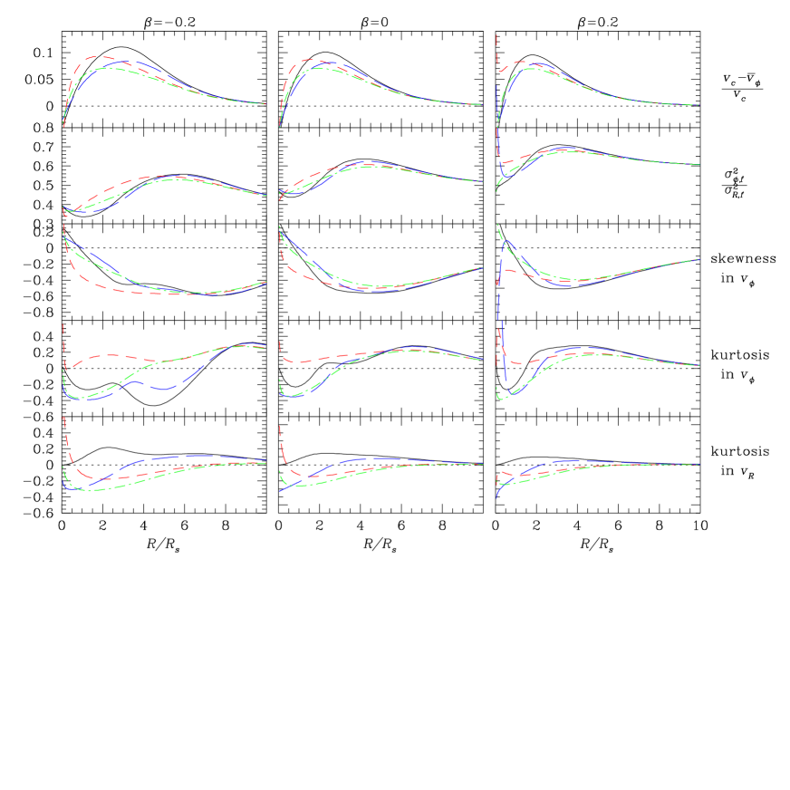
Figure 4: Kinematics vs. $R$ for the warm-disk DFs ${f_{\rm Shu}}$ (solid), ${f_{\rm new}}$ (dashed), ${f_{\rm a}}$ (dot-dashed), and ${f_{\rm b}}$ (long dashed) for an exponential disk with $R_{\sigma}{\,{=}\,}3R_{\Sigma}$ and $\sigma_{0}{\,{=}\,}0.5v_{0}$ in a slightly falling ($\beta{\,{=}\,}{-}0.2$), flat ($\beta{\,{=}\,}0$), and slightly rising ($\beta{\,{=}\,}0.2$) rotation curve (same as in Fig. 1a,b,c).

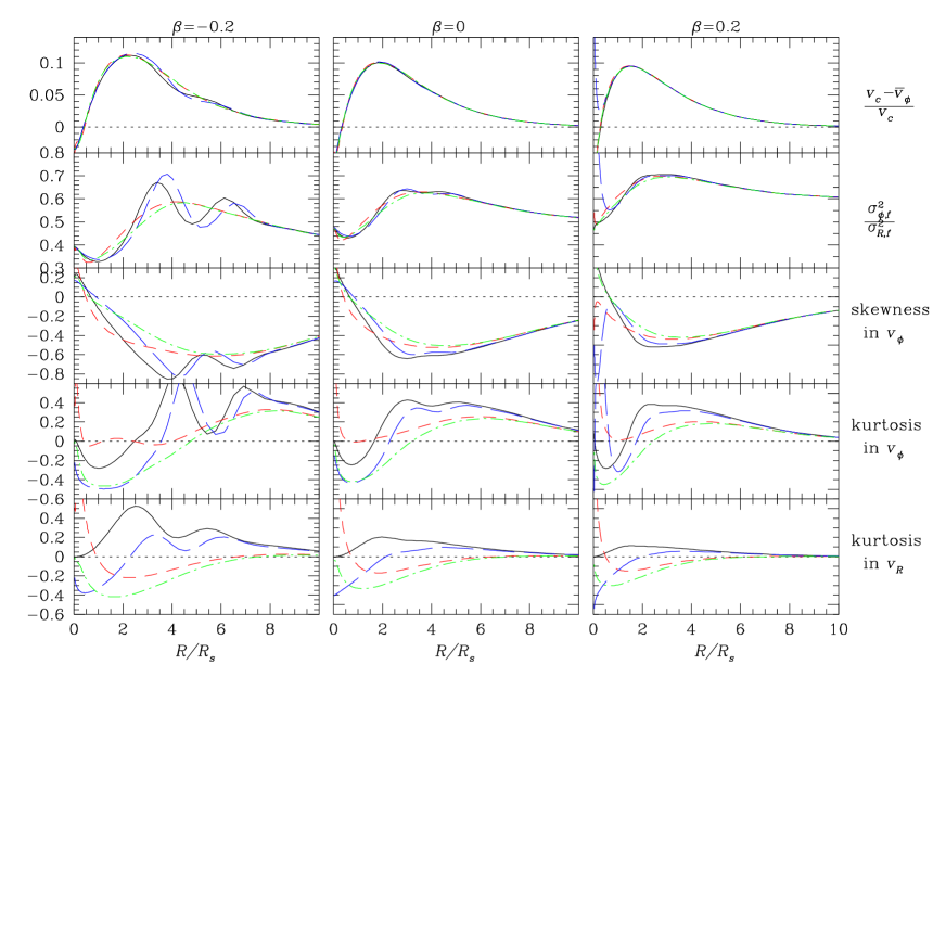
Figure 5: Same as Figure 4 but for DFs after four iterations of the algogithm of §3.2.1.

It seems, that after a few iterations no further improvement is achieved, i.e. the algorithm does converge to a model that definitely deviates from the target functions. For modest velocity dispersions this deviation is less than about one per cent, but up to a few per cent or even more, depending on the DF, for stellar disks with significant random motions. From our explanation for the algorithm below, this is not astonishing, since the algorithm is very crude indeed; on the contrary, it is suprising that it works so well.

3.2.2 Why Does This Algorithm Work?

The simple algorithm given above can be derived as follows. The integrations over velocity space that yield the moments may be cast into the form

$$\Sigma_{f}(R) = \int\Sigma^{\prime}(R_{1})\;K_{\Sigma}(R|R_{1})\,{\rm d}R_{1},$$ (16)

$$\mu_{f}(R) = \int\mu^{\prime}(R_{1})\;K_{\mu}(R|R_{1})\,{\rm d}R_{1}$$ (17)

with $\mu{\,{\equiv}\,}\sigma_{R}^{2}\Sigma$. The kernels $K_{\Sigma}$ and $K_{\mu}$ are implicitly defined by the form of the DF, but cannot be obtained explicitly. However, epicycle theory tells us that these Kernels should have a typical width of order $\sigma_{R}^{\prime}(R_{1})/\kappa(R_{1})$, which in turn is of the order $(\sigma_{R}^{\prime}/v_{c})_{R_{1}}R_{1}$. Equation (3.2.2) defines an inverse problem for finding the primed quantities given the unprimed ones. Clearly, to yield a physical meaningful DF, the primed quantites must not become negative, and a simple technique to solve for $\Sigma^{\prime}$ and $\sigma_{R}^{\prime}$ whilst ensuring positive definiteness is the Richardson-Lucy algorithm. This consists of iterating on (3.2.2) and the correction step

$$\Sigma^{\prime}(R_{1}) \rightarrow \Sigma^{\prime}(R_{1})\times\int{\Sigma(R)\over\Sigma_{f}(R)}\,K_{\Sigma}(R|R_{1})\,{\rm d}R,$$ (18)

$$\mu^{\prime}(R_{1}) \rightarrow \mu^{\prime}(R_{1})\times\int{\mu(R)\over\mu_{f}^{2}(R)}\,K_{\mu}(R|R_{1})\,{\rm d}R.$$ (19)

The algorithm given above emerges when replacing the kernels in (3.2.2) with $\delta$-functions. Clearly, this is a very crude simplification, but computing the integrals in (3.2.2) is non-trivial, and furthermore, the scheme works reasonably well, as demonstrated above.

4 THE KINEMATICS

As mentioned in the introduction, the distribution function $f(E,L)$ for a stellar disk is not uniquely specified by its surface density, velocity dispersion, and the gravitational potential. Rather, there is an infinite number of possible distribution functions with identical $\Sigma_{f}$ and $\sigma_{R,f}$, but with differences in, e.g., other velocity moments. Here, we will study the kinematics, i.e. the velocity moments up to order four, that emerge from the various warm-disk DFs when applied to the same stellar disk.

fig:kinem fig:kinem-iter

For the case of an exponential disk with $R_{\sigma}{\,{=}\,}3R_{\Sigma}$ and $\sigma_{0}{\,{=}\,}0.5v_{0}$ (as in Fig. 1a-c), Figure 4 plots various kinematical quantities resulting from the four different DFs of §2. Figure 5 differs only in that the DFs are those obtained after four iterations of the algorithm of §3.2.1. Obviously, in some cases this rather crude algorithm tends to create DFs with somewhat“ragged” kinematics.

The top panels show the run of the asymmetric drift velocity, which usually peaks between 1 and 2 $R_{\Sigma}$ for these models. The iterated DFs show almost identical behavior in their asymmetric drifts.

The second panels from top show the ratio between the kinetic energies in azimuthal and radial random motions, which in the solar neighborhood is measured to be about 0.42 (cf. Dehnen & Binney 1998). In the limit of small velocity dispersions, we know from Oort’s work that

$$\lim_{\sigma\to 0}\;{\sigma_{\phi}^{2}\over\sigma_{R}^{2}}={1\over 2}\left[1+{{\rm d}\ln v_{c}\over{\rm d}\ln R}\right]={-B\over A-B}=\gamma^{-2},$$ (20)

where $A$ and $B$ are Oort’s constants. Indeed, at large $R$, this value is reached by the moments of the DFs. However, at radii $R{\,{\ga}\,}2R_{\Sigma}$, all four DFs predict $\sigma_{\phi}^{2}/\sigma_{R}^{2}$ to be significantly larger than this limit. This is a known result for exponential disks (cf. [Evans & Collett 1993, Cuddeford & Binney 1994]). As the third panels from top of Figures 4 and 5 show, the $v_{\phi}$ distributions are always signicantly skewed in the sense that they have a low-$v_{\phi}$ tail. This tail is caused by stars originating from $R_{1}{\,{<}\,}R$ with large eccentricities – because of the exponential $\Sigma(R)$ and $\sigma_{R}(R)$ relations, there are many fewer stars with large eccentricity originating from $R_{1}{\,{>}\,}R$, which would create a high-$v_{\phi}$ tail. Such a skewness in the azimuthal motions is indeed observed in the solar neighborhood, cf. Dehnen (1998).

It is only in the kurtoses, i.e. moments of the fourth order, that the four DFs appear to differ significantly. While the kurtosis for the azimuthal motion is mostly positive, that of the radial motion may have either sign.

5 SAMPLING OF PHASE-SPACE POINTS

For $N$-body simulations and similar studies, it is of importance to draw phase-space points $(R,\dot{R},\phi,\dot{\phi})_{i},\,i=0,\dots N$ from the distribution function. One is often interested not in randomly distributed phase-space points but in a more regular distribution, where the points are equidistant in the phases (angle variables). Such a distribution has minimal noise, a fact important in numerical studies of stability properties (“quiet start” technique).

From the general form (13) of the warm-disk DFs presented, it is straightforward to derive a procedure for sampling $(E,L)$ as follows. First, determine $R_{1}$ according to $\Sigma(R)$, and translate it to either $E{\,{=}\,}E_{c}(R_{1})$ or $L{\,{=}\,}L_{c}(R_{1})$ according to the functional form of the DF. Second, sample the exponential in radial action and compute the remaining integral: $E$ or $L$. Here is a general algorithm that allows for parameter functions $\Sigma^{\prime}$ and $\sigma^{\prime}$ different from the targets and accurately corresponds to the DFs of §2.

• Choose a radius $R$ randomly from the cumulative distribution

  $$P(R)=\int_{0}^{R}R^{\prime}\,\Sigma(R^{\prime})\,{\rm d}R^{\prime}$$ (21)

  and determine $L{\,{=}\,}L_{c}(R)$ for ${f_{\rm Shu}}$ and ${f_{\rm b}}$ or $E{\,{=}\,}E_{c}(R)$ for ${f_{\rm new}}$ and ${f_{\rm a}}$. Evaluate the correction factor $g_{1}=\Sigma^{\prime}(R)/\Sigma(R)$.

  In the case of ${f_{\rm b}}$, the sign of $L$ must be chosen to be positive or negative with relative probabilities

  $$1:\exp\big{[}-2\Omega(R_{1})|L|/\sigma^{2}_{R}(R_{1})\big{]}.$$

• Choose $\xi\in(0,1)$ randomly and determine

  $$\begin{array}[]{r@{\,=\,}l@{\qquad{\rm for}\;\;}l}E&E_{c}(L)-\sigma^{\prime 2}_{R}(R)\ln\xi&{f_{\rm Shu}},\\[4.30554pt] L&L_{c}(E)+\sigma^{\prime 2}_{R}(R)\ln\xi\,/\Omega(R)&{f_{\rm new}},\\[4.30554pt] L&L_{c}\!\big{(}E+\sigma^{\prime 2}_{R}(R)\ln\xi\big{)}&{f_{\rm a}},\\[4.30554pt] E&E_{c}\!\big{(}|L|-\sigma^{\prime 2}_{R}(R)\ln\xi\,/\Omega(R)\big{)}&{f_{\rm b}}.\end{array}$$ (22)

  If $E\not\in[\Phi(0),\Phi(\infty)]$ or $L\not\in[-L_{c}(E),L_{c}(E)]$, go back to step 1 for another try.

• Integrate the orbit with these values of $(E,L)$ over one radial period $T_{R}$, compute $\omega_{R}(E,L)\equiv 2\pi/T_{R}$, and evaluate the correction factor $g_{2}{\,{=}\,}\kappa(R)/\omega_{R}(E,L)$.

• Sample $N_{\rm sam}$ phase-space points randomly from $\phi\in[0,2\pi)$ and $t\in[0,T_{R})$, use a table made during orbit integration to obtain $R(t)$ and $\dot{R}(t)$; $\dot{\phi}{\,{=}\,}L/R^{2}$. Here $N_{\rm sam}$ is either of the two integers next to $g_{1}\,g_{2}\,N_{\rm orb}$, chosen with probabilities such that the mean is equal to $g_{1}\,g_{2}\,N_{\rm orb}$.

• Iterate steps 1 to 4 until the desired number $N$ of points is sampled.

Here, $N_{\rm orb}$ is, approximately, the number of points chosen per orbit, and is usually between 1 and $N^{1/2}$. If noise is to be minimized, e.g. if initial conditions for a quiet start are needed, use $N_{\rm orb}{\,{\gg}\,}1$ and quasi-random numbers or even equidistant points, otherwise pseudo-random numbers. If only $(E,L)$ shall be sampled, set $N_{\rm orb}{\,{=}\,}1$. Note that for ${f_{\rm Shu}}$ and ${f_{\rm b}}$ the correction factor $g_{2}$ can become quite large for eccentric orbits, since these DFs are based on estimating $\omega_{R}$ by $\kappa(L)$, which goes to infinity as $L\to 0$ in centrally non-harmonic potentials, as, e.g., in the Milky Way. In the case of ${f_{\rm b}}$, one first determines $|L|$ and has to choose the sign afterwards.

I have checked the correctness of the above algorithm numerically by computing $\Sigma_{f}$ and $\sigma_{Rf}$ from $10^{6}$ sampled phase-space points: they agreed within their statistical uncertainties with the results from direct numerical integration.

6 CONCLUSION

6.1 Summary

Distribution functions for dynamically warm stellar disks may be considered as warmed-up versions of completely cold disks, in which all stars rotate on circular orbits. In fact, this picture for the DF of a stellar disk may be considered a good description for its formation history. In Section 2, I presented four different functional forms for warm-disk DFs $f(E,L)$, given the gravitational potential $\Phi(R)$ and prescriptions for the surface-density and velocity-dispersion profiles, $\Sigma(R)$ and $\sigma_{R}(R)$. One of them, ${f_{\rm Shu}}$, was introduced by Shu in 1969 and has already been used in studies, e.g. of the solar neighborhood kinematics (see Bienaymé 1999 for a recent example). The other three DFs have not been described in the literature so far.

In Section 3, the surface-density and velocity-dispersion profiles produced by the DFs as moments were compared to the target profiles. The comparison shows that, for a typical case reminiscent to the old stellar disk in the Milky Way, Shu’s DF, ${f_{\rm Shu}}$ results in the largest deviations between moments and targets, while the new DF (10) gives deviations that are about three times smaller. This new DF even gives an useful model when the stellar disk is dynamically hot within about one scale radius. Actually, the deviation of the moments from the target profiles $\Sigma(R)$ and $\sigma_{R}(R)$ may be considerably reduced by allowing the corresponding parameter functions appearing in the definition of the DFs to differ from these targets. In Section 3.2, a simple algorithm for this purpose is presented, which after only four iteration reduces the deviations in $\Sigma$ and $\sigma_{R}$ to well below 1 per cent for a typical case. Again, the DF ${f_{\rm new}}$ is best suited for this game, as it leads to the smallest deviations also in the iterated case. Another advantage of ${f_{\rm new}}$ is that is naturally extends to negative $L$, while ${f_{\rm Shu}}$ make the rather unnatural assumption that there are no stars with $L{\,{<}\,}0$.

In Section 4, I have compared the velocity moments up to fourth order of the four DFs iterated and non-iterated. For all four DFs, the ratio of azimuthal to radial velocity dispersion squared, $\sigma^{2}_{\phi}/\sigma^{2}_{R}$ is significantly larger than $\case{1}{2}[1{\,{+}\,}{\rm d}\ln v_{c}/{\rm d}\ln R]$ for $R$ larger than about 2 disk scale radii. The value $\case{1}{2}[1{\,{+}\,}{\rm d}\ln v_{c}/{\rm d}\ln R]$ is expected from Oort’s equation (20), which in turn is based on the epicycle approximation whereby ignoring the strong gradients in an exponential disk. In the solar neighborhood, $\sigma^{2}_{\phi}/\sigma^{2}_{R}\approx 0.42$ is observed, i.e. smaller than what we expect for a near-flat rotation curve. This deviation must be caused by a wrong assumption in the models, most likely that of axisymmetry – an investigation in terms of the influence of the Galactic bar is the subject of a future paper.

Finally, in Section 5, I give an algorithm for the sampling of phase-space points $(R,p_{R},\phi,L)$ from any one of the four DFs. This should be particularly useful for the creation of initial conditions for $N$-body simulations, either of the evolution of disk galaxies (bar formation, warps, etc.) or of mergers involving disk galaxies.

6.2 Thick Disks

An obvious extension of the thin-disk DFs presented in this paper are DFs describing stellar disks with some finite thickness. For this purpose, one needs a handle on the vertical motion of the stellar orbits. Unfortunately, typical three-dimensional axisymmetric potentials generally do not support a global third integral of motion $I_{3}$, even though most orbits are regular. There are various ways of different sophistication which can be used to proceed. First, the most basic and in principle only wholly correct procedure is Schwarzschild’s (1979) method of modeling a stellar system as superposition of individual orbits, which are obtained by numerical integration. Second, one may ignore the details of the phase-space structure and obtain a global third integral by perturbation techniques or torus fitting. In this case, (13) can be generalized to

$$f\approx{f_{1}(R_{1})\over\sigma_{R}^{2}(R_{1})\,\sigma_{z}^{2}(R_{1})}\,\exp\!\left[-{\omega_{R}J_{R}\over\sigma^{2}_{R}(R_{1})}-{\omega_{z}J_{z}\over\sigma^{2}_{z}(R_{1})}\right]$$ (23)

with the vertical action $J_{z}$ ([Binney 1987, Dehnen & Binney 1996]). Third, one may use the vertical energy

$$E_{z}\equiv\case{1}{2}v_{z}^{2}+\Phi(R,z)-\Phi(R,0)$$

for $I_{3}$. This approach is presumably still very good for many applications, since $E_{z}$ is conserved to reasonable accuracy for many disk stars (but not for halo stars). Finally, one may restrict the analysis to a potential of Stäckel form, such that a globally valid $I_{3}$ explicitly exists for all orbits (see Bienaymé, 1999, for a recent application of this technique).

6.3 Computer Programs Available

The computer programs that I have designed in the course of this study are written in C++ and contain the following features.

• A general concept for one-dimensional potentials and several implementations (power-law, $\gamma$-models, Isochrone) are given. Among other things, this contains routines for numerical orbit integration and evaluation of $J_{R}$, $\omega_{R}$, and $\omega_{\phi}$.

• A general concept of warm-disk DFs of the form (13) is given, which allows for integration of general velocity moments $\overline{\Sigma v_{R}^{m}v_{\phi}^{n}}{\,{\equiv}\,}\!\int{\rm d}^{2}\!\mbox{\boldmath$v$}\,v_{R}^{m}v_{\phi}^{n}f$. It also enables computation of $f(E,L)$, $R_{1}(E,L)$, and the derivatives of $f$ w.r.t. the parameter functions $\Sigma^{\prime}$ and $\sigma_{R}^{\prime}$ (useful for fitting $f$ to some data).

• Code for sampling phase-space points from a DF either pseudo- or quasi-randomly (the latter to reduce noise) according to the algorithm given in Section 5.

• The iterative algorithm of Section 3.2.1 to improve the match between moments and targets is implemented.

These programs are electronically available from me upon request. There is also an interface which allows one to use a reduced version of these routines from C programs.

References

- [Binney 1987] Binney J.J., 1987, in The Galaxy, eds. Gilmore & Carswell (Dordrecht: Reidel), 339
- [Bienaymé 1999] Bienaymé O., 1999, A&A, 341, 86
- [Cuddeford & Binney 1994] Cuddeford P., Binney J.J., 1994, MNRAS, 266, 273
- [Dehnen & Binney 1996] Dehnen W., Binney J.J., 1996, in Formation of the Galactic Halo … Inside and Out, eds. Morrison & Sarajedini, ASP Conf. Ser. 92, 393
- [Dehnen & Binney 1998] Dehnen W., Binney J.J., 1998, MNRAS, 298, 387
- [Dehnen 1998] Dehnen W., 1998, AJ, 115, 2384
- [Dehnen 1999] Dehnen W., 1999, AJ, 000, 000, paper I (astro-ph/9906081)
- [Evans & Collett 1993] Evans N.W., Collett J.L., 1993, MNRAS, 264, 353
- [Hunter & Qian 1993] Hunter C., Qian E., 1993, MNRAS, 262, 401
- [Kalnajs 1976] Kalnajs A., 1976, ApJ, 205, 751
- [Schwarzschild 1979] Schwarzschild M., 1979, ApJ,232, 236
- [Shu 1969] Shu F.H., 1969, ApJ, 158, 505