Correlated adiabatic and isocurvature perturbations from double inflation

Abstract

It is shown that double inflation (two minimally coupled massive scalar fields) can produce correlated adiabatic and isocurvature primordial perturbations. Depending on the two relevant parameters of the model, the contributions to the primordial perturbations are computed, with special emphasis on the correlation, which can be quantitatively represented by a correlation spectrum. Finally the primordial spectra are evolved numerically to obtain the CMBR anisotropy multipole expectation values. It turns out that the existence of mixing and correlation can alter very significantly the temperature fluctuation predictions.

I Introduction

In our present picture, cosmological fluctuations today are seen as the combination of an initial spectrum, which can be computed within the framework of high energy models (like inflation), with the subsequent processes occuring at lower energy where the physics is believed to be better understood (up to some unknowns such as the amount and nature of dark matter, the mass of neutrinos…). In the near future, we expect new and precise information on cosmological fluctuations with the planned measurements of the Cosmic Microwave Background Radiation (CMBR) anisotropies by the satellites MAP [1] and PLANCK [2]. It has been emphasized in the recent years that the precision of these measurements could in principle allow us to determine with a high precision the cosmological parameters [3]. These studies however all assume very simple initial perturbations, typically Gaussian adiabatic perturbations with a power-law spectrum. However, reality could turn out to be more subtle. This then would have the drawback to complicate the determination of the cosmological parameters but could open the fascinating perspective to gain precious information on the primordial universe. At present, at a time when data are still unprecise, it is essential to identify broad categories of early universe models and to determine their specificities as far as observable quantities are concerned, with the purpose to be able to discriminate between these various classes of models when detailed data will become available.

Ultimately, inflation must be related to a high energy physics model. Today there are many viable models but a generic feature of these models is that they contain generally many scalar fields. A property of inflation with several scalar fields is that it can generate, in addition to the ubiquitous adiabatic perturbations, isocurvature perturbations. In this respect, it is important to consider the possible role of primordial isocurvature perturbations. Isocurvature perturbations are perturbations in the relative density ratio between various species in the early universe, in contrast with the more standard adiabatic (or isentropic) perturbations which are perturbations in the total energy density with fixed particle number ratios. Primordial isocurvature perturbations are, most of the time, ignored in inflationary models. The main reason for this is that they are less universal than adiabatic perturbations because, on one hand, they can be produced only in multiple inflationary models [4], and, on the other hand, they can survive until the present epoch only if at least one of the inflaton fields remains decoupled from ordinary matter during the whole history of the universe. However, not only the existence of isocurvature perturbations is allowed in principle, but candidates for inflatons with the required above conditions even exist in many theoretical models (dilatons, axions).

What has already been established is that a pure isocurvature scale-invariant spectrum must be rejected because it predicts on large scales too large temperature anisotropies with respect to density fluctuations [5]. But other possibilities can be envisaged. Several have been investigated in the literature: tilted isocurvature perturbations [6], combination of isocurvature and adiabatic perturbations [7]. In the latter case, only combinations of independent isocurvature and adiabatic perturbations were considered. The aim of this paper is to investigate the possibility of correlated mixtures of isocurvature and adiabatic perturbations.

To illustrate this, the simplest model of multi-field inflation is considered here: double inflation [8], namely a model with two massive scalar fields without self-interaction or mutual interaction (other than gravitational). The production of fluctuations in this model has been studied in great detail by Polarski and Starobinsky and, in the present work, their notation and formalism will be followed closely. They were interested essentially in adiabatic perturbations [9] (see also [10] for a numerical analysis) but also considered isocurvature perturbations [11]. However, they did not investigate the range of parameters where this model has the striking property to produce correlated isocurvature and adiabatic perturbations. By this, we mean the cases where both isocurvature and adiabatic perturbations receive significant contributions of at least one of the scalar fields, in contrast to the uncorrelated case where one of the scalar fields feeds essentially the adiabatic perturbations while the second one is at the origin of the isocurvature perturbations.

The plan of this paper is the following. In section 2, the model of double inflation will be presented. Section 3 will be devoted to the analysis of adiabatic and isocurvature perturbations: their definition, how they are obtained from the inflation perturbations, the conditions to obtain correlated mixtures. Section 4 considers formally the definition of spectra for the perturbations as well as the notion of correlation. In section 5, the predictions for the CMBR anisotropies and matter power spectrum are given for the models with correlated primordial perturbations.

II Double inflation

As mentioned in the introduction, inflation needs at least two scalar fields to produce isocurvature perturbations. That is why we investigate the simplest model of inflation with two scalar fields: they are non-interacting, massive, minimally coupled scalar fields. The Lagrangian corresponding to this model is

$${\cal L}={{}^{(4)}R\over 16\pi G}-{1\over 2}\partial_{\mu}\phi_{l}\partial^{\mu}\phi_{l}-{1\over 2}m^{2}_{l}\phi^{2}_{l}-{1\over 2}\partial_{\mu}\phi_{h}\partial^{\mu}\phi_{h}-{1\over 2}m_{h}^{2}\phi^{2}_{h},$$ (1)

where the subscripts $l$ and $h$ designate respectively the light and heavy scalar fields (and thus $m_{h}>m_{l}$). ${}^{(4)}R$ is the scalar spacetime curvature and G Newton’s constant.

A The background equations

In a spatially flat Friedmann-Lemaître-Robertson-Walker (FLRW) spacetime, with metric $ds^{2}=-dt^{2}+a^{2}(t)d\vec{x}^{2}$, the equations of motion read

$$3H^{2} = 4\pi G(\dot{\phi}_{l}^{2}+\dot{\phi}_{m}^{2}+m_{l}^{2}\phi^{2}_{l}+m_{h}^{2}\phi^{2}_{h})$$ (2)

$$\ddot{\phi}_{l} + 3H\dot{\phi}_{l}+m^{2}_{l}\phi_{l}=0,$$ (3)

$$\ddot{\phi}_{h} + 3H\dot{\phi}_{h}+m^{2}_{h}\phi_{h}=0.$$ (4)

Following [9] it is convenient, during the phase when both scalar fields are slow-rolling (i.e. when $\dot{\phi}_{l}^{2}$ and $\dot{\phi}_{h}^{2}$ can be neglected in (2), $\ddot{\phi}_{l}$ and $\ddot{\phi}_{h}$ in (4)), to write the evolution of the two scalar fields in the following parametric form

$$\phi_{h}=\sqrt{s\over 2\pi G}\sin\theta,\qquad\phi_{l}=\sqrt{s\over 2\pi G}\cos\theta$$ (5)

where

$$s=-\ln(a/a_{e})$$ (6)

is the number of e-folds between a given instant and the end of inflation. This form (5) is a consequence of the approximate relation $d(\phi_{h}^{2}+\phi_{l}^{2})/ds=-d(\phi_{h}^{2}+\phi_{l}^{2})/(Hdt)\simeq(2\pi G)^{-1}$ resulting from the (slow-roll) equations of motion. The angular variable $\theta$ can then be related to the parameter $s$ by the expression

$$s=s_{0}{(\sin\theta)^{2\over R^{2}-1}\over(\cos\theta)^{2R^{2}\over R^{2}-1}}$$ (7)

where $R$ is the ratio of the masses of the two scalar fields

$$R\equiv{m_{h}\over m_{l}}.$$ (8)

The equation (7) was obtained by integrating the relation giving $d\theta/d(\ln s)$ as a function of $\theta$, which can be established by use of the slow-roll approximation of the equations of motion (2)-(4) (see [9] for the details of the calculations). As noticed in [9], equation (7) can be approximated, when $\theta\gg R^{-1}$, by the simple formula

$$s\simeq{s_{0}\over\cos^{2}\theta}.$$ (9)

This behaviour corresponds to the period when inflation is dominated by the heavy scalar field (this approximation is valid as long as $s>s_{0}$ and $s-s_{0}\gg s_{0}/R^{2}$). This period ends when $\theta\sim R^{-1}$, $s\sim s_{0}$ and is followed (possibly after a dust-like transition period) by a phase of inflation dominated by the light scalar field.

It follows from (2)-(5) that the Hubble parameter can be expressed in the form

$$H^{2}(s)\simeq{2\over 3}m^{2}_{l}s[1+(R^{2}-1)\sin^{2}\theta(s)],$$ (10)

where the function $\theta(s)$ is obtained by inverting (7) ($0<\theta<\pi/2$). As inflation proceeds, $s$ decreases and $\theta$ goes to smaller and smaller values, which implies a decreasing Hubble parameter during inflation.

It will be convenient to define $s_{H}$ as the number of e-folds before the end of inflation when the scale corresponding to our Hubble radius today crossed out the Hubble radius during inflation. The value of $s_{H}$ depends on the temperature after the reheating (see e.g. [12] ) but roughly $s_{H}\simeq 60$. To make definite calculations, we shall take throughout this work the value

$$s_{H}=60.$$ (11)

Note that the class of models considered here depends on three free parameters: the two masses $m_{l}$ and $m_{h}$, or alternatively $m_{l}$ and $R$, and the parameter $s_{0}$. In particular, the choice of this last parameter $s_{0}$ relatively to $s_{H}$ will determine the specific phase of double inflation, ‘heavy’ dominated, intermediate or ‘light’ dominated, during which the perturbations on scales of cosmological relevance were produced.

B Perturbations

After having determined the evolution of the background quantities, let us turn now to the evolution of the linear perturbations. We shall restrict our analysis to the so-called scalar perturbations (in the terminology of Bardeen [13]). We thus consider a spacetime linearly perturbed about the flat FLRW spacetime of the previous subsection, endowed with the metric

$$ds^{2}=-(1+2\Phi)dt^{2}+a^{2}(t)(1-2\Psi)\delta_{ij}dx^{i}dx^{j}.$$ (12)

Although this metric is not the most general a priori, it turns out that any perturbed metric (of the scalar type) can be transformed into a metric of this form by a suitable coordinate transformation. This choice corresponds to the so-called longitudinal gauge. In addition to the geometrical perturbations $\Phi$ and $\Psi$, one must also consider the matter perturbations, which will simply be during inflation the perturbations of the scalar fields, respectively $\delta\phi_{h}$ and $\delta\phi_{l}$, with respect to their homogeneous values.

Before writing down the equations of motion for the perturbations, it is convenient to use a Fourier decomposition and to define the Fourier modes of any perturbed quantity $f$ by the relation

$$f_{{\bf k}}=\int{d^{3}{\bf x}\over(2\pi)^{3/2}}e^{-i{\bf k}.{\bf x}}f({\bf x}).$$ (13)

The equations of motion for the perturbations are derived from the perturbed Einstein equations and from the Klein-Gordon equations of the scalar fields. They lead to the following four equations (see e.g. [14])

$$\Phi=\Psi,$$ (14)

$$\dot{\Phi}+H\Phi=4\pi G\left(\dot{\phi}_{h}\delta\phi_{h}+\dot{\phi}_{l}\delta\phi_{l}\right),$$ (15)

$$\ddot{\delta\phi_{h}}+3H\dot{\delta\phi_{h}}+\left({k^{2}\over a^{2}}+m_{h}^{2}\right)\delta\phi_{h}=4\dot{\phi}_{h}\dot{\Phi}-2m_{h}^{2}\phi_{h}\Phi,$$ (16)

$$\ddot{\delta\phi_{l}}+3H\dot{\delta\phi_{l}}+\left({k^{2}\over a^{2}}+m_{l}^{2}\right)\delta\phi_{l}=4\dot{\phi}_{l}\dot{\Phi}-2m_{l}^{2}\phi_{l}\Phi,$$ (17)

where the subscript ${\bf k}$ is here implicit, as it will be throughout this paper.

In the slow-rolling approximation and for superhorizon modes, i.e. $k\ll aH$, these equations can be solved (see [9]) and the dominant solutions read

$$\Phi\simeq-{C_{1}\dot{H}\over H^{2}}+2C_{3}{(m_{h}^{2}-m_{l}^{2})m_{h}^{2}\phi_{h}^{2}m_{l}^{2}\phi_{l}^{2}\over 3(m_{h}^{2}\phi_{h}^{2}+m_{l}^{2}\phi_{l}^{2})^{2}},$$ (18)

$${\delta\phi_{l}\over\dot{\phi}_{l}}\simeq{C_{1}\over H}-2C_{3}{Hm_{h}^{2}\phi_{h}^{2}\over m_{h}^{2}\phi_{h}^{2}+m_{l}^{2}\phi_{l}^{2}},\quad{\delta\phi_{h}\over\dot{\phi}_{h}}\simeq{C_{1}\over H}+2C_{3}{Hm_{l}^{2}\phi_{l}^{2}\over m_{h}^{2}\phi_{h}^{2}+m_{l}^{2}\phi_{l}^{2}},$$ (19)

where $C_{1}({\bf k})$ and $C_{3}({\bf k})$ are time-independent constants of integration and are fixed by the initial conditions. As usual in inflation, perturbations are assumed to be initially (i.e. before crossing out the Hubble radius) in their vacuum quantum state. Perturbations outside the Hubble radius are then obtained by amplification of the vacuum quantum fluctuations due to the gravitational interaction. The two scalar fields being independent, one simply duplicates the results of single scalar field inflation (see e.g. [14]). Consequently, $\delta\phi_{h}$ and $\delta\phi_{l}$ can be written, for wavelengths crossing out the Hubble radius, as

$$\delta\phi_{h}={H_{k}\over\sqrt{2k^{3}}}e_{h}({\bf k}),\quad\delta\phi_{l}={H_{k}\over\sqrt{2k^{3}}}e_{l}({\bf k}),$$ (20)

where $e_{h}$ and $e_{l}$ are classical Gaussian random fields with $\langle e_{i}({\bf k})\rangle=0$, $\langle e_{i}({\bf k})e_{j}^{*}({\bf k}^{\prime})\rangle=\delta_{ij}\delta({\bf k}-{\bf k}^{\prime})$, for $i,j=l,h$, and $H_{k}$ is the Hubble parameter when the mode crosses the Hubble radius, i.e., when $k=2\pi aH$. Neglecting the evolution of the Hubble parameter with respect to that of the scale factor, the number of e-folds $s_{k}$ corresponding to the instant when the mode of wavenumber $k$ crossed out the Hubble radius, is given simply by

$$k\simeq k_{H}e^{s_{H}-s_{k}},$$ (21)

where $k_{H}$ is the wavenumber corresponding to the present Hubble scale. In the present work, our interest will focus on the scales of cosmological relevance, typically $k/k_{H}\simeq 0.1-2000$. This means that the range of e-folds that will interest us is $52\lesssim s_{k}\lesssim 63$.

III Primordial perturbations

The analysis of the solutions for the perturbations during inflation obtained in the previous section will now enable us to determine the “initial” (but post-inflationary) conditions for the perturbations in the radiation era taking place after inflation and reheating.

A Initial conditions in the radiation era

At some past instant deep in the radiation era, we shall consider four species of particles. Two species will be relativistic: photons and neutrinos; two species will be non-relativistic: baryons and cold dark matter. Their respective energy density contrasts will be denoted ${\delta}_{\gamma}$, ${\delta}_{\nu}$, ${\delta}_{b}$ and ${\delta}_{c}$ (${\delta}_{A}\equiv{\delta}\rho_{A}/\rho_{A}$).

At this point, it is useful to define precisely the notion of adiabatic and isocurvature perturbations. Isocurvature pertubations are defined by the condition that there is no perturbation of the energy density in the total comoving gauge (denoted by the subscript $(c)$), i.e.

$$\sum_{A}{{\delta}^{(c)}}\rho_{A}=0,$$ (22)

but that there are perturbations in the ratios of species particle numbers, i.e.

$${\delta}^{(c)}(n_{A}/n_{B})\neq 0$$ (23)

in general. By contrast, adiabatic (or isentropic) perturbations are defined by the prescription that the particle number ratios between various species is fixed, i.e.

$${\delta}^{(c)}(n_{A}/n_{B})=0,$$ (24)

whereas the total energy density perturbation can fluctuate, i.e.

$$\sum_{A}{{\delta}^{(c)}}\rho_{A}\neq 0.$$ (25)

It is clear from the above definitions that, if one considers N species, there will be in general one adiabatic mode and $N-1$ isocurvature modes. Here, it will be assumed that the light scalar field $\phi_{l}$ decays into ordinary particles, i.e. gives birth to the photons, neutrinos and baryons, while the dark matter particles are associated exclusively with the heavy scalar field $\phi_{h}$. Note that part of the dark matter could be also produced by the light scalar field but we shall ignore this possiblity here for simplicity. As a consequence, the particle number ratios between the three ‘ordinary’ species will be frozen, i.e.

$${{\delta}^{(c)}n_{\gamma}\over n_{\gamma}}={{\delta}^{(c)}n_{\nu}\over n_{\nu}}={{\delta}^{(c)}n_{b}\over n_{b}},$$ (26)

and only one isocurvature mode will exist, which can be conveniently represented by the quantity

$$S\equiv{{\delta}^{(c)}n_{c}\over n_{c}}-{{\delta}^{(c)}n_{\gamma}\over n_{\gamma}}={\delta}^{(c)}_{c}-{3\over 4}{\delta}^{(c)}_{\gamma}.$$ (27)

Going back to the longitudinal gauge, and following Ma and Bertschinger [15], one can write the initial conditions deep in the radiation era for modes outside the Hubble radius in the form

$${\delta}_{\gamma}=-2\Phi,$$ (28)

$${\delta}_{b}={3\over 4}{\delta}_{\nu}={3\over 4}{\delta}_{\gamma},$$ (29)

$${\delta}_{c}=S+{3\over 4}{\delta}_{\gamma},$$ (30)

$$\theta_{\gamma}=\theta_{\nu}=\theta_{b}=\theta_{c}={1\over 2}(k^{2}\eta)\Phi,$$ (31)

$$\sigma_{\nu}={1\over 15}(k\eta)^{2}\Phi,$$ (32)

$$\Psi=\left(1+{2\over 5}R_{\nu}\right)\Phi,$$ (33)

with $R_{\nu}=\rho_{\nu}/(\rho_{\gamma}+\rho_{\nu})$ and where $\theta$ stands for the divergence of the fluid three-velocity, $\sigma_{\nu}$ for the shear stress of neutrinos (in the rest of this paper, the contribution of neutrinos in all analytical calculations will be ignored for simplicity but it will be taken into account in the numerical calculations) and $\eta$ is the conformal time defined by $d\eta=dt/a(t)$. All the information about the initial conditions is thus contained in the two k-dependent quantities $\Phi$ and $S$, which are time-independent during the radiation era (for $k\ll aH$). The next subsections will be devoted to make the link between these two quantities and the perturbations during inflation.

B Adiabatic initial perturbations

The evolution of $\Phi$ is given by (18) only during the phase when both scalar fields are slow rolling. As soon as the heavy scalar field $\phi_{h}$ ends its slow-rolling phase, the second term on the right hand side of (18) will die out, and $\Phi$ can be given during all the subsequent evolution of the universe in the simple form

$$\Phi=C_{1}\left(1-{H\over a}\int_{0}^{t}a(t^{\prime})dt^{\prime}\right).$$ (34)

It can be checked that, during inflation, $1-{H\over a}\int_{0}^{t}a(t^{\prime})dt^{\prime}\simeq-\dot{H}/H^{2}$, which ensures that the coefficient $C_{1}$ in the above formula is the same as in (18).

It is thus essential to express $C_{1}$ in terms of the perturbations of the two scalar fields, and therefore in terms of $e_{l}$ and $e_{h}$, in order to be able to determine the amplitude of the perturbations after the end of inflation. Combining the two equations in (19) and using (20), as well as the slow-roll approximation of the background equations of motion (2)-(4), the expression for the coefficient $C_{1}$ during inflation is found to be

$$C_{1}({\bf k})\simeq-{4\pi G}{H_{k}\over\sqrt{2k^{3}}}\left[\phi_{l}e_{l}({\bf k})+\phi_{h}e_{h}({\bf k})\right].$$ (35)

As it is clear from this formula, $C_{1}(k)$ is a stochastic variable, whose properties can be determined from the stochastic properties of $e_{l}$ and $e_{h}$.

During the radiation era, the relation between the coefficient $C_{1}$ and the gravitational potential is simply, using once more (34),

$$\Phi={2\over 3}C_{1}({\bf k}).$$ (36)

Therefore, the gravitational potential during the radiation era for modes larger than the Hubble scale is given by the expression [9]

$$\hat{\Phi}\simeq-{4\sqrt{\pi G}\over 3}k^{-3/2}\sqrt{s_{k}}H_{k}\left[\sin\theta_{k}e_{h}({\bf k})+\cos\theta_{k}e_{l}({\bf k})\right],$$ (37)

where $H_{k}$ is given as a function of $s_{k}$ in (10) and $s_{k}$ is given as a function of $k$ in (21). The hat in the above equations (and in all subsequent equations) indicates that the value of the corresponding quantity is taken deep in the radiation era when the wavelength of the Fourier mode is larger than the Hubble radius.

C Isocurvature initial perturbations

As explained in subsection A, the isocurvature perturbations in the present model are due to variations in the relative proportions of cold dark matter, generated by the heavy scalar field, with respect to the three other main species (photons, baryons, neutrinos), all generated by the light scalar field. Moreover, during the radiation era, the isocurvature perturbation $S$ rigorously defined by (27) is essentially the comoving cold dark matter density contrast, $S\simeq{\delta}^{(c)}_{c}$, so that what is needed to obtain the primordial isocurvature spectrum is simply to compute the cold dark matter density contrast in terms of the scalar field perturbations during inflation. This task was carried out in [11]. Only the main points will be summarized here.

Let us first give the comoving energy density perturbation associated with the heavy scalar field:

$${\delta}\rho_{h}^{(c)}=\dot{\phi}_{h}{\delta}\dot{\phi}_{h}+m_{h}^{2}\phi_{h}{\delta}\phi_{h}+3H\dot{\phi}_{h}{\delta}\phi_{h}-\dot{\phi}_{h}^{2}\Phi.$$ (38)

Matching the inflationary phase when $\phi_{h}$ is slow-rolling to the the inflationary phase when $\phi_{h}$ is oscillating and then to the post-reheating radiation dominated phase, one finds [11]

$${\delta}_{h}^{(c)}\simeq-{4\over 3}m_{h}^{2}C_{3}.$$ (39)

The coefficient $C_{3}$ can then be obtained, during inflation, by substracting the two equations in (19) and then using the (slow-roll) background equations of motion and (20). Inserting the result in (39), the density contrast of the cold dark matter (associated with the heavy scalar field), for modes larger than the Hubble radius, is found to be given, during the radiation era, by the expression

$${\delta}_{h}^{(c)}\simeq\sqrt{2\over k^{3}}H_{k}\left(\phi_{h}^{-1}e_{h}({\bf k})-{m_{h}^{2}\over m_{l}^{2}}\phi_{l}^{-1}e_{l}({\bf k})\right),$$ (40)

where the value of the scalar fields is taken at Hubble radius crossing. This can be reexpressed, using (5) and (8), in the form

$$\hat{S}\simeq{\delta}_{h}^{(c)}\simeq 2\sqrt{\pi G}k^{-3/2}s_{k}^{-1/2}H_{k}\left[{e_{h}\over\sin\theta_{k}}-{R^{2}\over\cos\theta_{k}}e_{l}\right].$$ (41)

Note that the isocurvature perturbations have the same power-law dependence as the adiabatic perturbations multiplied by a weakly k-dependent expression which is different from the analogous expression in (37).

D Conditions for the existence of correlated adiabatic and isocurvature perturbations

As shown above, the quantities describing the primordial adiabatic and isocurvature perturbations are in general linear combinations of the independent stochastic quantities $e_{l}$ and $e_{h}$ and are thus expected to be correlated. It is now necessary to examine the actual value of the corresponding coefficients. For adiabatic perturbations, i.e. in equation (37), the light contribution is dominant for $\tan\theta<1$ whereas the heavy contribution is dominant for $\tan\theta>1$. For isocurvature perturbations, i.e. in equation (41), the light contribution dominates for $\tan\theta>R^{2}$ whereas the heavy contribution is predominant in the opposite case. Assuming $R^{2}\gg 1$, one can thus divide the space of parameters for double inflation into three regions:

1 Region $\tan\theta>>1$

The adiabatic perturbations are dominated by the heavy scalar field while the isocurvature perturbations are dominated by the light scalar field. The two types of perturbations will thus appear independent. Moreover, except for $\theta$ very close to $\pi/2$, the isocurvature amplitude will be suppressed with respect to the adiabatic amplitude by a factor $s_{k}$. In this parameter region, one recovers the standard results of a pure adiabatic spectrum due to a single scalar field, here the heavy scalar field.

2 Region $\tan\theta<<R^{-2}$

In this region, essentially only the light scalar field contributes to the adiabatic perturbations while the isocurvature perturbations are dominated by the heavy scalar field. The two contributions are therefore independent and the isocurvature amplitude can be very high with respect to the adiabatic one if $\theta$ is sufficiently small.

3 Region $R^{-2}\leq\tan\theta\leq 1$

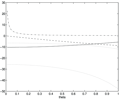
This is the most interesting region. Here, both the adiabatic and isocurvature perturbations are essentially feeded by the fluctuations of the light scalar field (even if their amplitude depends on the background value of the two scalar fields). This means that the adiabatic and isocurvature perturbations are strongly correlated in this region. If one considers the relative magnitude of these light scalar field contributions, one sees that the isocurvature contribution can compensate the $s_{k}^{-1}$ suppression (with respect to the adiabatic perturbations) by a suitable factor $R^{2}$. Note also that in the upper part of this parameter region, i.e. for $\tan\theta\lesssim 1$, the heavy and light contributions in the adiabatic perturbations will be of similar order while the heavy contribution in the isocurvature perturbations can be ignored. In contrast, in the lower part of the region, i.e. $\theta\sim R^{-2}$, the heavy contribution in the adiabatic perturbations is negligible whereas the light and heavy contributions in the isocurvature perturbations are of similar weight. This is illustrated on Figure 1, which displays the relative behaviour of the four contributions as a function of the angle $\theta$.

The expressions for the adiabatic and isocurvature primordial perturbations, (37) and (41) can be simplified further when one assumes that these perturbations are produced during some specific phases of inflation. For instance, if all scales of cosmological relevance are produced during the period of inflation dominated by the heavy scalar field, then the approximate relation (9) relating the angle $\theta$ to the number of e-folds applies, which enables us to simplify the Hubble parameter expression, given in equation (10), into

$$H(s)\simeq\sqrt{2\over 3}m_{l}\sqrt{R^{2}-1}\sqrt{s-s_{0}}.$$ (42)

The various contributions to adiabatic and isocurvature perturbations then reduce to the form

$$k^{3/2}\hat{\Phi}_{h}\simeq-{4\sqrt{6\pi G}\over 9}m_{l}\sqrt{R^{2}-1}\left(s_{k}-s_{0}\right),\quad k^{3/2}\hat{\Phi}_{l}\simeq-{4\sqrt{6\pi G}\over 9}m_{l}\sqrt{R^{2}-1}\sqrt{s_{0}\left(s_{k}-s_{0}\right)},$$ (43)

and

$$k^{3/2}\hat{S}_{h}\simeq{2\sqrt{6\pi G}\over 3}m_{l}\sqrt{R^{2}-1},\quad k^{3/2}\hat{S}_{l}\simeq-{2\sqrt{6\pi G}\over 3}m_{l}R^{2}\sqrt{R^{2}-1}\sqrt{s_{k}-s_{0}\over s_{0}},$$ (44)

where the indices $h$ and $l$ refer to the corresponding coefficients of $e_{h}$ and $e_{l}$ in (37) and (41). Let us briefly comment these results when one varies the free parameters of the model, $m_{l}$, $R$ and $s_{0}$ (but remaining in the domain of validity of the above approximate expressions). Considering the variations with respect to the first two parameters, one can notice that all the contributions are proportional to the term $m_{l}\sqrt{R^{2}-1}$, except $\hat{S}_{l}$ which contains an additional $R^{2}$ dependence. This means, ignoring for the moment the (weak) scale dependence, that the relative amplitudes of three of the contributions are fixed, the relative amplitude of $\hat{S}_{l}$ being adjustable by the mass ratio $R$. Once $R$ is fixed, the overall amplitude of the perturbations can be fixed by the scale $m_{l}$. Concerning now the variation of the contributions with the cosmological scale, $\hat{S}_{h}$ is scale-invariant, while the three other are weakly scale dependent: $\hat{\Phi}_{l}$ and $\hat{S}_{l}$ have the same dependence, whereas $\hat{\Phi}_{h}$ has a stronger dependence.

Another limiting case corresponds to $\theta\ll R^{-1}$, which occurs during the period of inflation dominated by the light scalar field. In this case, one has $s\simeq s_{0}\theta^{2/R^{2}}$ and the Hubble parameter is approximately given by

$$H(s)\simeq\sqrt{2\over 3}m_{l}\sqrt{s}.$$ (45)

As a consequence, the ’heavy’ and ’light’ contributions are approximated by

$$k^{3/2}\hat{\Phi}_{h}\simeq-{4\sqrt{6\pi G}\over 9}m_{l}s_{k}\theta_{k},\quad k^{3/2}\hat{\Phi}_{l}\simeq-{4\sqrt{6\pi G}\over 9}m_{l}s_{k}$$ (46)

for the adiabatic perturbations and

$$k^{3/2}\hat{S}_{h}\simeq{2\sqrt{6\pi G}\over 3}m_{l}\theta_{k}^{-1},\quad k^{3/2}\hat{S}_{l}\simeq-{2\sqrt{6\pi G}\over 3}m_{l}R^{2}$$ (47)

for isocurvature perturbations. The ’heavy’ adiabatic contribution is thus negligible and the perturbations due to the heavy scalar field are therefore essentially isocurvature.

Note, to conclude this section, that in their work [9], Polarski and Starobinsky, concentrated their attention on the intermediate case where the scales of cosmological relevance just correspond to the transition zone from the heavy scalar field driven inflation to the light scalar field driven inflation. As a consequence, their spectrum has a stronger variation in $k$ than in the limiting cases considered above. Here, the emphasis is put on contributions to the isocurvature perturbations. With another choice of parameters, one can also produce a huge temperature anisotropy dipole due to isocurvature perturbations on scales larger than the present Hubble radius [16].

IV Spectra and correlation of adiabatic and isocurvature perturbations

A General definitions

It is usually assumed in cosmology that the perturbations can be described by (homogeneous and isotropic) gaussian random fields. In the specific model under consideration here, where the perturbations are created during an inflationary phase, this is true by construction. What is new here is that isocurvature and adiabatic perturbations are not assumed to be independent. Indeed, as shown in the previous section, in the case of double inflation, the two kinds of perturbations are correlated, at least for some region of the parameter space. It will thus be our purpose to define statistical quantities that can describe random fields which are, a priori, correlated. Let us first recall, for any homogeneous and isotropic random field $f$, the standard definition (up to a normalization factor) of its power spectrum by the expression

$$\langle f_{{\bf k}}f_{{\bf k}^{\prime}}^{*}\rangle=2\pi^{2}k^{-3}{\cal P}_{f}(k)\delta({\bf k}-{\bf k}^{\prime}).$$ (48)

In addition to this definition, it will be useful to define a covariance spectrum between two random fields $f$ and $g$ by the following expression

$${\cal R}e\langle f_{\bf k}g^{*}_{{\bf k}^{\prime}}\rangle=2\pi^{2}k^{-3}{\cal C}_{f,g}(k)\delta({\bf k}-{\bf k}^{\prime}).$$ (49)

In order to estimate the degree of correlation between two quantities, it is convenient to also define the correlation spectrum ${\tilde{\cal C}}_{f,g}(k)$ by normalizing ${\cal C}_{f,g}(k)$:

$${\tilde{\cal C}}_{f,g}(k)={{\cal C}_{f,g}(k)\over\sqrt{{\cal P}_{f}(k)}\sqrt{{\cal P}_{g}(k)}}.$$ (50)

Schwartz inequality implies, as usual, that $-1\leq{\cal C}_{f,g}(k)\leq 1$. The correlation (anticorrelation) will be stronger as one is closer to $1$ or $-1$.

B Double inflation generated perturbations

Let us now specialize the above formulas to the case of perturbations generated by double inflation. By substituting the explicit expressions for the perturbations obtained in the previous section, namely (37) and (41), one finds

$${\cal P}_{\hat{\Phi}}={8G\over 9\pi}H_{k}^{2}s_{k}$$ (51)

for the initial adiabatic spectrum,

$${\cal P}_{\hat{S}}={2G\over\pi}{H_{k}^{2}\over s_{k}}\left[{R^{4}\over\cos^{2}\theta}+{1\over\sin^{2}\theta}\right],$$ (52)

for the initial isocurvature spectrum and

$${\cal C}_{\hat{\Phi},\hat{S}}={4G\over 3\pi}H_{k}^{2}(R^{2}-1)$$ (53)

for the covariance spectrum. Combining the three above spectra according to (50), one finds finally for the correlation spectrum the expression

$${\tilde{\cal C}}_{\hat{\Phi},\hat{S}}={(R^{2}-1)\sin{2\theta}\over 2(R^{4}\sin^{2}\theta+\cos^{2}\theta)^{1/2}}.$$ (54)

It is instructive to study the dependence of this correlation spectrum with respect to the parameters of the model. If one takes $\theta$ fixed, one sees that the correlation will vanish for $R=1$ and will then increase monotonously with increasing $R$ approaching the asymptotic value $\cos\theta$. If now one considers $R$ as fixed and study the variations of the correlation with respect to $\theta$, one recovers the conclusions of section 3D: the correlation vanishes when $\theta$ approaches zero or $\pi/2$; inbetween, one can see that the correlation reach a maximum for $\sin^{2}\theta=(R^{2}+1)^{-1}$, with the value

$${\tilde{\cal C}}_{\hat{\Phi},\hat{S}}^{max}={R^{2}-1\over R^{2}+1}.$$ (55)

The correlation spectrum ${\tilde{\cal C}}_{\hat{\Phi},\hat{S}}$ for various choices of parameters has been plotted on Fig. 2, as a function of $s_{k}$. One can, as before, distinguish between the two extreme cases. For models such that $\theta\gg R^{-1}$, corresponding to a ’heavy’ inflationary phase, the various contributions vary slowly with $\theta$, as can be seen from Fig. 1. This means that the correlation will be almost constant. For models such that $\theta\ll R^{-1}$, corresponding to a ’light’ inflationary phase, $\hat{S}_{h}$ increases quickly with decreasing $\theta$, i.e. with decreasing scales, which implies that the correlation will decrease with decreasing scales, i.e. smaller $s_{k}$. The models with $s_{0}<s_{H}$ belong to the first category, while models with $s_{0}>s_{H}$ correspond to the second. Finally, the models with $s_{0}$ close to $s_{H}$ have an intermediate behaviour between the two extreme cases. They also have the strongest correlation.

V Predictions for the CMBR and density contrast spectrum

A Analytical predictions for long-wavelength perturbations

1 Evolution of the perturbations

In the case of perturbations whose wavelength is larger than the Hubble radius, the time evolution is particularly simple. For an initial isocurvature perturbation characterized by the initial amplitude $\hat{S}$, the entropy perturbation $S$ is unchanged as long as the perturbation is larger than the Hubble radius, whatever the evolution of the backgroung equation of state, i.e.

$$S=\hat{S}\qquad(k\ll aH).$$ (56)

However, the radiation-matter transition will generate a gravitational potential perturbation (see e.g. [12])

$$\Phi^{iso}=-{1\over 5}\hat{S}\qquad(k\ll aH).$$ (57)

Of course, the initial adiabatic perturbation will also contribute to the gravitational potential perturbation:

$$\Phi^{ad}=T\hat{\Phi}\qquad(k\ll aH),$$ (58)

where $T$ is a coefficient, close to $1$, due to the evolution of the universe (if one ignores the anisotropic stress of the neutrinos, $T=9/10$.)

2 Large angular scale CMBR anisotropies.

At large angular scales, the temperature anisotropies are essentially due to the sum of an intrinsic contribution and of a Sachs-Wolfe [17] contribution. Except for the dipole for which the Doppler terms are important, the Sachs-Wolfe contribution can be written (for a spatially flat background)

$$\left(\Delta T\over T\right)_{SW}({\bf e})={1\over 3}\Phi(x_{ls});$$ (59)

Where ${\bf e}$ on the left hand side is a unit vector corresponding to the direction of observation and $x_{ls}$ on the right hand side represents the intersection of the last scattering surface with the light-ray of direction ${\bf e}$. The intrinsic contribution is simply given, via the Stefan law, as the perturbation ${\delta}^{(c)}_{\gamma}/4$ at the time of last scattering. Since last scattering occured in the matter era, ${\delta}^{(c)}_{m}\simeq{\delta}^{(c)}$, and therefore for an adiabatic perturbation (${\delta}^{(c)}_{m}={3\over 4}{\delta}^{(c)}_{\gamma}$), $\left({\Delta T}\over T\right)_{\rm int}\simeq{1\over 3}{\delta}^{(c)}_{m}$, which can be seen to be negligible (see below (62)) with respect to the Sachs-Wolfe contribution, whereas for an isocurvature perturbation ($S\simeq-{3\over 4}{\delta}^{(c)}_{\gamma}$ during matter era),

$$\left(\Delta T\over T\right)_{int}\simeq-{1\over 3}S.$$ (60)

To conclude, the temperature anisotropies will be given in general by

$${\Delta T\over T}={1\over 3}T\hat{\Phi}-{2\over 5}\hat{S}$$ (61)

on angular scales larger than the angle (of the order of the degree) corresponding to the size of the Hubble radius at the time of the last scattering. This equation enables us to estimate easily the normalization of the temperatures anisotropies for the low multipoles (see the definition (68)-(69)), essentially constrained by COBE measurements. Note that for mixed primordial perturbations with isocurvature and adiabatic contributions of the same order of magnitude, the low multipoles anisotropies can be significantly reduced by a compensation effect between the isocurvature perturbation and the adiabatic one. It turns out that this is the case for the light scalar field contribution in double inflation models with $R\sim 5$ (see Fig.1 and the consequence on Fig. 3-5).

3 Large scale structure

Large scale structure is governed by the density contrast, or equivalently the gravitational potential perturbation $\Phi$ since the latter quantity can be related to the (total) contrast density in the comoving gauge by the (generalized) Poisson equation, which reads (see e.g. [14])

$$\left({k\over aH}\right)^{2}\Phi=-{3\over 2}{\delta}^{(c)}.$$ (62)

For modes inside the Hubble radius the evolution becomes quite complicated and depends on the specific ingredients of the model. But what is relevant for our purpose is that this subhorizon evolution does not depend on the nature of the primordial perturbations. What matters is the total gravitational potential perturbation $\Phi$ which can be written, in the matter era, as

$$\Phi=\Phi_{ad}-{1\over 5}S.$$ (63)

Note that the influence of primordial isocurvature perturbations is smaller on the large scale density power spectrum (see (63)) than on large scale temperature anisotropies (see (61)).

4 Spectra

Using the relation (61) (with $T=1$), the spectrum for the large scale temperature anisotropies can be expressed in terms of the primordial isocurvature and adiabatic spectra,

$${\cal P}_{{\Delta T\over T}}={1\over 9}{\cal P}_{\hat{\Phi}}+{4\over 25}{\cal P}_{\hat{S}}-{4\over 15}{\cal C}_{\hat{\Phi},\hat{S}}.$$ (64)

When only primordial adiabatic perturbations are present, the previous expression implies

$${\cal P}^{1/2}_{\Delta T\over T}={1\over 3}{\cal P}^{1/2}_{\Phi},$$ (65)

whereas for pure isocurvature perturbations, one finds

$${\cal P}^{1/2}_{\Delta T\over T}=2{\cal P}^{1/2}_{\Phi}.$$ (66)

This is in agreement with the standard comment in the literature that isocurvature perturbations generate CMBR anisotropies six times bigger than equivalent adiabatic perturbations. This is the reason why isocurvature perturbations are in general rejected in comological models [5]. However, when one takes into account both isocurvature and adiabatic perturbations, with the possibility of correlation, then the additional term due to correlation can change significantly these conclusions. Illustrations will be given in the next subsection.

Similarly, the spectrum for the gravitational potential is given by

$${\cal P}_{\Phi}={\cal P}_{\hat{\Phi}}+{1\over 25}{\cal P}_{\hat{S}}-{2\over 5}{\cal C}_{\hat{\Phi},\hat{S}}.$$ (67)

B All-scale predictions

After having considered long wavelength perturbations, whose advantage is one can estimate analytically their observable amplitude and thus normalize easily the models, let us analyze now smaller scales, which require the use of numerical computation.

1 CMBR anisotropies

As it is customary, one decomposes the CMBR anisotropies on the basis of spherical harmonics:

$${\Delta T\over T}(\theta,\phi)=\sum_{l=1}^{\infty}\sum_{m=-l}^{l}a_{lm}Y_{lm}(\theta,\phi).$$ (68)

The predictions of a model are usually given in terms of the expectation values of the squared multipole coefficients

$$C_{l}\equiv\langle|a_{lm}|^{2}\rangle.$$ (69)

In the present model, the temperature anisotropies will be the superposition of a contribution due to the heavy scalar field and of a contribution due to the light scalar field. These two contributions are independent, because the stochastic quantities $e_{h}$ and $e_{l}$ are independent, and as such the coefficients $C_{l}$ can be decomposed

$$C_{l}=C_{l}^{(l)}+C_{l}^{(h)},$$ (70)

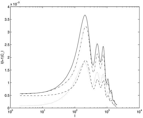
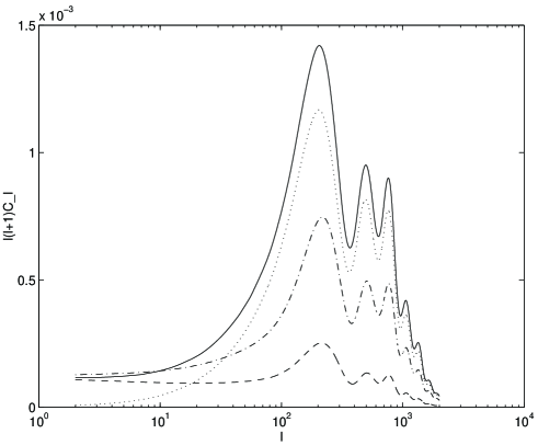
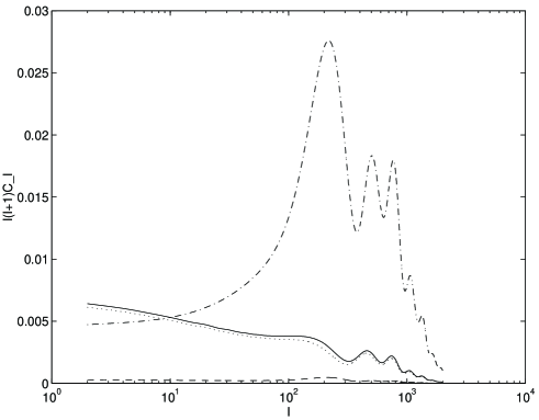
where the upper index refers to the ’light’ or ’heavy’ nature of the perturbations. It is important to emphasize that only a decomposition of this type is allowed here. For example, a decomposition of the $C_{l}$ as a sum of an isocurvature contribution and of an adiabatic contribution would be wrong here. In practice, the heavy and light contributions to the $C_{l}$ are computed independently, by using twice a Boltzmann code (developped in our group by A. Riazuelo, and used in [18]). The first run takes as initial condition $\hat{\Phi}_{h}$ and $\hat{S}_{h}$ and yields the coefficients $C_{l}^{(h)}$. Similarly, the second run computes the $C_{l}^{(l)}$ using as initial conditions the corresponding quantities $\hat{\Phi}_{l}$ and $\hat{S}_{l}$. The results for $C_{l}^{(l)}$ and $C_{l}^{(h)}$, as well as their sum $C_{l}$, are plotted on Fig. 3-6 for four illustrative models (for all models the Hubble parameter and the baryon density correspond respectively to $h_{100}=0.5$, $\Omega_{b}=0.052$). For the first three models, the value $R=5$ has been chosen because the isocurvature and adiabatic contributions of the light scalar field are then of similar amplitude, as is visible on Fig. 1, and the effects of mixing and correlation are particularly important. A consequence of the similar amplitude (with the same sign) of the two ‘light’ contributions is an important suppression of the light spectrum $C_{l}^{(l)}$ for small $l$, as noticed already in the previous subsection, and as is visible on Fig 3-5. In contrast, one can check on Fig. 6 that this will not be the case for the $R=10$ model, for which $\hat{S}_{l}$ is dominant.

The first two graphs have a roughly similar behaviour for the ’heavy’ contribution. What distinguishes them is the ’light’ contribution, which illustrates its high sensitivity on the relative amplitudes of $\hat{S}_{l}$ and $\hat{\Phi}_{l}$. A systematic investigation of the effects of mixed correlated primordial spectra, independently of the early universe model to produce them, on the temperature anisotropies will be given elsewhere [19]. For these two models, one notices an amplification (weak in the first case and strong in the second) of the main acoustic peak with respect to the standard (pure adiabatic and scale-invariant) model. In contrast, the third example shows a suppression of the main peak, which is due to a strong contribution $\hat{S}_{h}$, which makes the ’heavy’ spectrum look “isocurvature” and thus damps the main peak in the global spectrum. Finally, the last example is characteristic of the domination of the ‘light’ spectrum, itself dominated by the isocurvature contribution ($\hat{S}_{l}$), which thus makes the global spectrum look ”isocurvature”. It is rather remarkable that modest variations of the two relevant parameters of the model, $R$ and $s_{0}$ ($m_{l}$ is useful simply for an overall normalization of the parameters), can lead to a large variety of temperature anisotropy spectra.

C Power Spectrum

Another quantity which is extremely important for the confrontation of models with the observations is the (total) density power spectrum. In the literature, it is usually denoted $P(k)$ and its relation to the corresponding spectrum ${\cal P}_{{\delta}^{(c)}}$ (for the comoving density constrast) defined generically in (48) is

$$P(k)=2\pi^{2}k^{-3}{\cal P}_{{\delta}^{(c)}}.$$ (71)

Using the Poisson equation (62), it can be reexpressed in terms of the gravitational potential spectrum

$$P(k)={8\pi^{2}\over 9(a_{0}H_{0})^{4}}k{\cal P}_{\Phi}(k).$$ (72)

As with the temperature anisotropies, the power spectrum for double inflation is obtainable by computing independently the power spectrum for the heavy scalar field contribution, then that for the light scalar field contribution, and finally by adding the two results,

$$P(k)=P_{l}(k)+P_{h}(k).$$ (73)

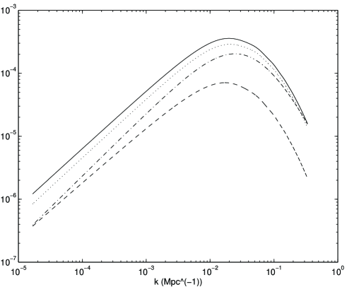
In contrast with the temperature anisotropies, the influence of the mixing and correlation of the primordial perturbations on the density spectrum is less spectacular because the shapes of the pure isocurvature and pure adiabatic density spectra are not extremely different. There is however a sensible difference: the pure isocurvature spectrum has, relatively to the large scales, less power on small scales than the pure adiabatic spectrum. To illustrate what happens for mixed and correlated primordial perturbations, Fig. 7 displays, for the model specified by the parameters $R=5$ and $s_{0}=50$, the total power spectrum , together with the two independent ‘light’ and ‘heavy’ contributions, as well as the standard adiabatic CDM power spectrum (normalized as before) for comparison. Note that the resulting spectrum has, relatively to large scales, less power than the standard adiabatic power spectrum. However, it has globally more power than the standard spectrum for the same temperature anisotropy amplitude on small $l$.

VI Conclusions

The main conclusion of this work is that it is possible, in the simplest model of multiple inflation, to obtain correlated isocurvature and adiabatic primordial perturbations. These perturbations slightly deviate from scale-invariance but their correlation can entail significant modifications with respect to standard single scalar field models.

This class of models, both simple and rich, could provide an interesting field of experiment to investigate the feasibility to determine the cosmological parameters and the primordial perturbations from expected data. The question would be, assuming Nature has chosen this particular model, could we infer from the expected temperature anisotropy data the cosmological parameters and to which precision? More important, would it possible to discriminate between a single field inflation model and a multiple field model with correlated perturbations and what would be the price to pay on the precision of the cosmological parameters ?

It was not the purpose of the present work to exhibit a model supposed to fit better the observations. However, one of these models, surprisingly, turns out to present two characteristics, which are at present favoured by observations: a power spectrum with modest power at small scales (comparatively to the standard CDM model) and a high peak on intermediate scales. It may be worth seeing how well this model does when confronted with the current observations.

Finally, it would be interesting to investigate the possiblity of correlated adiabatic and isocurvature perturbations within the framework of multiple inflation with interaction between scalar fields and see how the main features presented here would be modified.

FIG. 1.: Relative amplitude of the $\phi_{h}$ contributions to the adiabatic perturbations, $\hat{\Phi}_{h}$ (dashed line), to the isocurvature perturbations, $\hat{S}_{h}$ (dotted dashed line), and of the $\phi_{l}$ contribution to the adiabatic perturbations, $\hat{\Phi}_{l}$ (continuous line), and to the isocurvature perturbations, $\hat{S}_{l}$ (dotted line). The last quantity, the only one which depends on $R$, has been plotted for $R=5$ (upper dotted line) and $R=10$ (lower dotted line).

FIG. 2.: Correlation spectrum for various parameters. Continuous curves from bottom to top (on the left hand side of the figure) correspond respectively to $(R=5,s_{0}=30)$, $(R=5,s_{0}=50)$ and $(R=10,s_{0}=50)$. The dashed curve corresponds to $(R=5,s_{0}=60)$, the dotted dashed curve to $(R=5,s_{0}=70)$ and finally the dotted curve to $(R=5,s_{0}=80)$.

FIG. 3.: Temperature anisotropies for the double inflation scenario with $R=5$, $s_{0}=30$. The total anisotropies (continuous line) are the sum of a contribution due to the heavy scalar field (dashed line) and of a contribution of the light scalar field (dotted line). To make the comparison, the anisotropies due to standard (adiabatic scale-invariant) perturbations are also plotted (dotted dashed line), using $C_{10}$ for normalization.

FIG. 4.: Temperature anisotropies for the double inflation scenario with $R=5$, $s_{0}=50$ (same conventions as in Fig.3).

FIG. 5.: Temperature anisotropies for the double inflation scenario with $R=5$, $s_{0}=80$.

FIG. 6.: Temperature anisotropies for the double inflation scenario with $R=10$, $s_{0}=50$.

FIG. 7.: Power spectrum for the double inflation scenario with $R=5$, $s_{0}=50$. The total power spectrum (continuous line) is the sum of a contribution due to the heavy scalar field (dashed line) and of a contribution of the light scalar field (dotted line). The standard (adiabatic scale-invariant) power spectrum is also plotted (dotted dashed line) with the same normalization for $C_{10}$.