Abundances and Physical Conditions in the Warm Neutral Medium Towards $\mu$ Columbae

Abstract

We present ultraviolet interstellar absorption line measurements for the sightline towards the O9.5 V star $\mu$ Columbae ($l=237\fdg 3$, $b=-27\fdg 1$; $d\approx 400$ pc, $z\approx 180$ pc; $\langle n_{\rm HI}\rangle\approx 0.06$ cm^-3) obtained with the Goddard High Resolution Spectrograph (GHRS) on board the Hubble Space Telescope. These archival data represent the most complete GHRS interstellar absorption line measurements for any line of sight towards an early-type star. The 3.5 km s^-1 resolution of the instrument allow us to accurately derive the gas-phase column densities of many important ionic species in the diffuse warm neutral medium, including accounting for saturation effects in the data and for contamination from ionized gas along this sightline. We find that the effects of an H II region around $\mu$ Col itself do not significantly affect our derivation of gas-phase abundances. For the low velocity material ($-20\lesssim v_{\rm LSR}\lesssim+15$ km s^-1) we use the apparent column density method to derive column densities. For the individual absorbing components at $v_{\rm LSR}\approx-28.8$, $+20.1$, $+31.0$, and $+41.2$ km s^-1, we apply component fitting techniques to derive column densities and $b$-values. We have also used observations of interstellar Ly$\alpha$ absorption taken with the GHRS intermediate resolution gratings to accurately derive the H I column density along this sightline. The resulting interstellar column density $\log N(\mbox{{H~{}I}})=19.86\pm 0.015$ is in agreement with other determinations but is significantly more precise.

The low-velocity material shows gas-phase abundance patterns similar to the warm cloud (cloud A) towards the disk star $\zeta$ Ophiuchi , while the component at $v_{\rm LSR}\approx+20.1$ km s^-1 shows gas-phase abundances similar to those found in warm halo clouds. We find the velocity-integrated gas-phase abundances of Zn, P, and S relative to H along this sightline are indistinguishable from solar system abundances. We discuss the implications of our gas-phase abundance measurements for the composition of interstellar dust grains. We find a dust-phase abundance $\left[{\rm(Fe+Mg)}/{\rm Si}\right]_{d}=2.7-3.3$ in the low-velocity gas; therefore the dust cannot be composed solely of common silicate grains, but must also include oxides or pure iron grains. The low velocity material along this sightline is characterized by $T\approx 6,000-7,000$ K with $n_{e}\approx 0.3$ cm^-3, derived from the ionization equilibrium of Mg and Ca.

The relative ionic column density ratios of the intermediate velocity components at $v_{\rm LSR}=+31.0$ and $+41.2$ km s^-1 show the imprint both of elemental incorporation into grains and (photo)ionization. These clouds have low total hydrogen column densities ($\log N({\rm H})\sim 17.4-17.7$), and our component fitting $b$-values constrain the temperature in the highest velocity component to be $T=4,000\pm 700$ K. The electron density of this cloud is $n_{e}\approx 0.6$ cm^-3, derived from the ${}^{2}P_{1/2}$ to ${}^{2}P_{3/2}$ fine structure excitation of C II. The components at $v_{\rm LSR}\approx-30$ and $-48$ km s^-1 along this sightline likely trace shocked gas with very low hydrogen column densities. The $v_{\rm LSR}\approx-30$ km s^-1 component is detected in a few strong low-ionization lines, while both are easily detected in Si III. The relative column densities of the $-30$ km s^-1 suggest the gas is collisionally ionized at moderate temperatures ($T\approx 25,000$ K). This is consistent with the measured $b$-values of this component, though non-thermal motions likely contribute significantly to the observed breadths.

1 INTRODUCTION

The measurement and analysis of interstellar absorption lines provides fundamental information on the content and physical conditions of the Galactic interstellar medium (ISM). In particular, measurements of the gas-phase abundances of the ISM have allowed us to infer the composition of interstellar dust and trace the variations in the dust make-up in a wide range of environments (e.g., Savage, Cardelli, & Sofia 1992; Spitzer & Fitzpatrick 1993, 1995; Sembach & Savage 1996; Lu et al. 1998). Furthermore, atomic absorption lines allow us to study the chemical evolutionary history of the Universe over 90% of its age through the study of gaseous QSO absorption lines (e.g., Lu et al. 1996; Pettini et al. 1997, 1999; Prochaska & Wolfe 1999), provided we can understand the imprint dust leaves on the measurements. The effects of dust are best constrained by our studies of gas-phase abundances at zero redshift.

The study of Galactic interstellar absorption lines has been greatly aided by the Goddard High Resolution Spectrograph (GHRS) on board the Hubble Space Telescope (HST). The echelle-mode resolution of this instrument (FWHM$\,\approx 3.5$ km s^-1) coupled with its ability to achieve high signal to noise ultraviolet observations of Galactic early-type stars makes it a very powerful instrument for studying absorption lines in the Galactic ISM.

The star $\mu$ Columbae is the GHRS high- and intermediate-resolution radiometric standard. As such, it was observed extensively during the Servicing Mission Orbital Verification (SMOV) stages after the installation of the Corrective Optics Space Telescope Axial Replacement (COSTAR). In the post-COSTAR era, more than 500 echelle-mode observations were made of $\mu$ Col using the GHRS, as well as a similar number of observations with the lower-resolution first-order gratings. This makes $\mu$ Col the most extensively observed early-type star with the GHRS.

The design of the GHRS calibration observations during the SMOV period were such that the extensive $\mu$ Col echelle-mode dataset is characterized by extensive wavelength coverage and relatively high signal-to-noise ratios. The resulting high-resolution absorption line dataset is almost ideal for studying abundances along the low-density sightline to this star. Though this sightline has been extensively studied by the Copernicus satellite (Shull & York 1977; hereafter SY) and with the pre-COSTAR GHRS by Sofia, Savage & Cardelli (1993; hereafter SSC), the extremely rich dataset acquired after the installation of COSTAR represents a significant increase in resolution over the observations of SY and in S/N over those of SSC. The extensive wavelength coverage of the dataset includes observations of a wide assortment of ionic species, with most being observed in several transitions with a range of $f$-values.

We have reduced and analyzed the extensive archival GHRS ultraviolet absorption line dataset for the $\mu$ Col sightline. Our main objectives in this work are to very accurately derive the gas-phase elemental abundances in the low- and intermediate-velocity gas along this sightline as well as information on the physical conditions of the gas. From the gas-phase abundances we infer the dust content of the ISM in this direction and discuss the implications of these data for understanding the make-up of dust grains in the diffuse ISM.

Our work is presented as follows. We discuss the properties of the $\mu$ Col sightline and the previous studies of this sightline in §2. In §3 we describe our reductions of the GHRS dataset, as well as our extraction and analysis methods for analyzing the ISM absorption line data. In §4 we discuss the gas-phase abundances of the low-velocity material along this sightline, including a detailed analysis of the contributions from an H II region about $\mu$ Col itself and the derivation of physical conditions for the absorbing gas. We present an analysis of the abundances of the intermediate velocity gas along this sightline in §5. A discussion of the implications of this interstellar absorption line dataset is included in §6, and we summarize our major conclusions in §7.

2 THE $\mu$ COL SIGHTLINE

The star $\mu$ Columbae (HD 38666) lies in the direction ($l,\ b$) = (237^∘, $-27^{\circ}$) along a relatively unreddened sightline [E($\bv$) = 0.02; Bastiaansen 1992]. Classified as an O9.5 V star by Walborn (1973), $\mu$ Col is a runaway star with a radial velocity relative to the local standard of rest (LSR) of $v_{\rm LSR}=+90$ km s^-1 (Gies 1987; Keenan & Dufton 1983). Lesh (1968) has placed the star as far away as 1000 pc. The absolute magnitude scale of Vacca, Garmany, & Shull (1996) yields a slightly smaller distance of $\approx 790$ pc, given the observed magnitude $V=5.16$. However, recent Hipparcos measurements have constrained its parallax to be $\pi=2.52\pm 0.55$ milliarcseconds (Perryman et al. 1997), implying a distance of only $400^{+100}_{-70}$ pc. This result is more consistent with the distance derived from Strömgren photometry (410 pc) by Keenan & Dufton (1983). This discrepancy in distance scale may be related to problems in assigning luminosity classes to rapidly rotating spectral standards (Lamers et al. 1997). We will adopt the Hipparcos results throughout this work, though the reader should be aware of the continuing gaps in our knowledge of the stellar distance scale.

The adopted distance, coupled with the observed neutral hydrogen column density of $\log N(\mbox{H$\;${\small\rm I}})=19.86\pm 0.015$ (see Appendix A), implies an average line of sight density of $\langle n_{\rm H}\rangle\approx 0.06$ cm^-3. Molecular hydrogen makes a negligible contribution to the total hydrogen column density with $\log N({\rm H_{2}})=15.50$ summed over $J=0$ to 4 (Spitzer, Cochran, & Hirshfeld 1975).

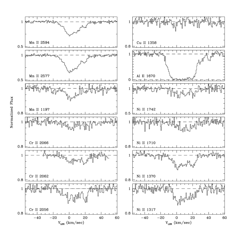
Figure 4: As Figure 1, but for the moderately to heavily depleted species Mn II, Cr II, Cu II, Al II, and Ni II.

Highly ionized gas along the $\mu$ Col sightline implies the presence of both hot ($T>10^{5}$ K) collisionally ionized material and photoionized gas near the star. York (1974) fit the strong interstellar O VI absorption along this sightline with a column density $\log N(\mbox{{O~{}VI}})=13.82\pm 0.02$ and a Doppler parameter $b_{\rm O\,VI}=43.8$ km s^-1. Brandt et al. (1999) present GHRS observations of weak C IV, Si IV and N V absorption at 3.5 km s^-1 resolution. Figures 1-7 show the normalized interstellar absorption line profiles for the $\mu$ Col sightline observed with the GHRS, including the profiles of C IV and Si IV (see Figure 6). The profile widths of the highly ionized atoms increase with ionization potential. The breadth of the profile implies $T<2\times 10^{6}$ K, while the width of the C IV line, for example, implies temperatures $T<2.3\times 10^{5}$ K; much of the velocity widths may be due to non-thermal motions. The O VI and C IV profiles are centered near $\langle v_{\rm LSR}\rangle=-2$ km s^-1, while the Si IV is centered at $\langle v_{\rm LSR}\rangle=+5$ km s^-1. The ratio $N(\mbox{{C~{}IV}})/N(\mbox{{O~{}VI}})=0.11\pm 0.01$ is consistent with that observed for other sightlines intercepting Galactic disk gas (Spitzer 1996). Brandt et al. suggest much of the O VI and some C IV arises in an evolved supernova remnant along the line of sight, though some of the high-ion absorption likely arises in the interface between the Local Cloud and the Local Bubble. They also show that a significant amount of the Si IV column density is likely produced in a low-density H II region surrounding $\mu$ Col. We will discuss in more detail the possible contributions of ionized gas to the absorption line measurements.

The low-ionization material along the sightline to $\mu$ Col was studied with the Copernicus satellite by SY at a resolution of $\approx 13$ km s^-1 and with the echelle gratings of the pre-COSTAR GHRS by SSC with a resolution of $\approx 3.5$ km s^-1. These studies have identified low-ion absorption in four main absorbing components, the properties of which are given in Table 1. This table includes the number by which we will refer to each of these absorbing regions, the approximate central velocity and the range of velocity over which the absorption from each region extends, both in the LSR frame, as well as the identifications of these regions in the nomenclature of SY and SSC. Regions 2, 3, and 4 are relatively well separated in velocity and may represent individual absorbing “clouds;” region 1 is a blend of several clouds that overlap in velocity. The region we designate as component 5, which appears at negative velocities, was described by SY as “trailing absorption.” Each of the absorbing regions in Table 1 shows different gas-phase abundances, suggesting changing patterns of elemental incorporation into dust grains and ionization. In general the absorption along this sightline is consistent with the Routly-Spitzer effect (Routly & Spitzer 1952), where the gas-phase abundances of refractory elements increase with velocity (SY; SSC; Hobbs 1978). Also given in Table 1 are the temperatures, $T$, and electron densities, $n_{e}$, for each component from our analysis below (see §4.4 and §5.3).

Lockman (1991) has discussed the H I 21-cm emission profile towards $\mu$ Col, which is reproduced in Figure 8. These data, from Lockman, Hobbs, & Shull (1986), have a 21′ beam and have been corrected for stray radiation. The column of H I from the 21-cm data is more than twice that derived from observations of Lyman-$\alpha$ along the sightline to $\mu$ Col, implying much of the H I column observed in 21-cm radiation comes from beyond the star. In the direction of $\mu$ Col Galactic rotation is expected to carry the gas to positive velocities, with a maximum velocity of $v_{LSR}\approx+5.2\pm 0.6$ km s^-1. The majority of the H I emission and the UV-absorption (i.e., the region 1 blend) resides at velocities allowed by Galactic rotation. A quite narrow component at $v_{\rm LSR}\approx 3$ km s^-1 shows the peak brightness temperature in the H I emission profile, though several broad absorbing clouds also contribute to the blend of region 1. It is clear that the H I content of components 2, 3, and 4 is significantly less than that of component 1. Though UV absorption profiles along this sightline show gas out to $v_{\rm LSR}\approx+42$ km s^-1, the H I emission profile shows an extended wing to $v_{\rm LSR}\gtrsim+60$ km s^-1.

Component 1 is centered at $v_{\rm LSR}\approx+3$ km s^-1 and contains $\sim 90\%$ of the neutral gas along the sightline, as evidenced by the relative strengths of the absorbing regions in the undepleted species S II. Ground based observations of the Na I D2 line at a resolution of 1 km s^-1 show the complex to consist of several (at least three or four) velocity components (Hobbs 1978; see Figure 8). Though the absolute velocity of the absorption is uncertain, SY tentatively associate the observed H₂ absorption with component 1.

The papers of SY and SSC have shown absorbing complex 1 likely has depletion characteristics similar to that of the warm cloud towards $\zeta$ Oph (component A of Savage et al. 1992). The low velocity resolution of the Copernicus data make the separation of absorption from components 1 and 2 difficult; the higher resolution observations of SSC are superior in this respect. Those elements with high condensation temperatures, such as Fe II and Cr II, exhibit gas phase abundances that are sub-solar with respect to S II by $\approx 1.3$ dex. Sofia et al. (SSC) suggest that the level of depletion exhibited by the $\mu$ Col component 1 and the warm component along the $\zeta$ Oph sightline may be typical of the low-density, warm neutral medium (WNM) of the Galactic disk.

The presence of ionized material in the velocity range encompassed by component 1 is suggested by N II and Si III absorption in the data of SY. The fine structure lines of N II^∗∗, which trace the densest ionized regions, are centered at $v_{\rm LSR}=0$ to +2 km s^-1. Shull & York argue that the majority of the ionized gas along the sightline is associated with an H II region surrounding $\mu$ Col and estimate a density $\langle n_{e}\rangle\approx 0.2$ cm^-3. Recent observations of this sightline with the WHAM Fabry-Perot spectrometer (Reynolds et al. 1998), which are reproduced in Figure 8, show that the ionized gas is indeed concentrated near $v_{\rm LSR}=0$ (M. Haffner, 1998, priv. comm.). The imprint of ionized regions on the column densities of (primarily) neutral gas tracers can be one of the largest uncertainties in studying the gas-phase abundances in the Galactic WNM, such as in component 1. We will discuss this contamination of our dataset in §4.1.

Component 2 appears distinctly in species that tend to be highly depleted in component 1. A quick comparison of the Ca II and Na I profiles of Hobbs (1978) shows that the ratio of these two species changes significantly as the velocity of the gas increases (these data are reproduced in Figure 8). This difference is likely due to the return of elements to the gas phase due to dust destruction. Shull & York (SY) and Sofia et al. (SSC) have shown that the refractory elements have a much higher relative abundance in this component than in the lower velocity material. This cloud is at a velocity that would place it well beyond the star if it were simply participating in Galactic rotation.

The intermediate-velocity gas along the $\mu$ Col sightline has been less-well observed due to the relatively low column of material present in these clouds. Centered at $v_{\rm LSR}\approx+33$ and +42 km s^-1, respectively, components 3 and 4 show patterns of abundances quite different than the low-velocity material. Both SY and SSC examine the gas-phase abundances in component 4, though component 3 was only identified by SSC. In both cases, the effects of ionization may be significant, though the gas-phase abundances of these clouds may also be high, suggesting substantial grain destruction (SSC). Shull & York also noted the presence of “trailing” absorption in the Si III profile. This material, which we identify as component 5, has a velocity relative to the local standard of rest $v_{LSR}\approx-30$ km s^-1, which is inconsistent with Galactic rotation.

Some $90\%$ of the gas towards $\mu$ Col is associated with component 1, which has velocities roughly consistent with expectations due to Galactic rotation. Most of the remaining 10% of the material has velocities which are inconsistent with rotation. Sembach & Danks (1994) have found that on average $\sim 10\%$ of Ca II absorption is at forbidden velocities. They estimate a cloud-to-cloud velocity dispersion in this forbidden-velocity gas of $\sigma\approx 22$ km s^-1. The forbidden-velocity gas towards $\mu$ Col, therefore, seems not to show highly unusual kinematics compared with the observations of low-density sightlines by Sembach & Danks.

3 DATA PROCESSING AND ANALYSIS

Table 2 lists basic information of the individual spectra used in our analysis of the $\mu$ Col sightline. The present set of observations was acquired for the purpose of evaluating the in-flight performance of and flux-calibrating the high-resolution modes of the GHRS following the installation of COSTAR. The data have been collected over a large span of time, beginning in early 1994 after the installation of COSTAR. As such, the observations do not represent a completely homogeneous data set. We rely most heavily on measurements made with the echelle-mode Ech-A and Ech-B gratings, which give a resolution of $\approx 3.5$ km s^-1 (FWHM). An extensive dataset exists for the first-order gratings as well, and we have used observations taken with the G140M and G160M gratings to derive the column densities of H I (see Appendix A) and Fe III along the $\mu$ Col sightline. Typically the star was observed for 30-120 seconds through the large science aperture (LSA; 1$\farcs$74$\times$1$\farcs$74) with four substeps per diode. Appropriate measurements were made of the inter-order scattered light in all cases (see Cardelli et al. 1993), and the observations employed the comb-addition routine with the on-board doppler compensator enabled. We have in general restricted ourselves to using the post-COSTAR data for this sightline due to the degradation in resolution of the pre-COSTAR LSA observations. We have, however, made use of pre-COSTAR small science aperture (SSA; 0$\farcs$22$\times$0$\farcs$22) data in our component fitting analysis (see §3.3.2).

3.1 Data Processing

Our calibration and reduction of the data follows procedures similar to those discussed in Savage et al. (1992) and Cardelli et al. (1995). Our determination and propagation of errors follows Sembach & Savage (1992) for our measurements of the integrated equivalent widths and column densities. The basic calibration was performed at the GHRS computing facility at the Goddard Space Flight Center and at the University of Wisconsin-Madison using the standard CALHRS routine. The CALHRS processing includes conversion of raw counts to count rates and corrections for particle radiation contamination, dark counts, known diode nonuniformities, paired pulse events and scattered light. The wavelength calibration was derived from the standard calibration tables and should be accurate to approximately $\pm 3.5$ km s^-1.

The final data reduction was performed using software developed and tested at the University of Wisconsin-Madison. This includes the merging of individual spectra and allowing for additional refinements to the scattered light correction. The inter-order scattered light removal discussed by Cardelli et al. (1990, 1993) is based upon extensive pre-flight and in-orbit analysis of GHRS data and is used by the CALHRS routine; the coefficients derived by these authors are appropriate for observations made through the SSA. We find that many of the LSA observations required an additional correction to bring the cores of strongly saturated lines to the appropriate zero level. The final scattered light coefficients, $d_{\rm c}$, used for each group of spectra are given in Table 2. Many of the observations had no strong lines which would allow us to refine the values of $d_{\rm c}$; those cases for which we have adopted the Cardelli et al. (1993) values, having no independent measure of $d_{\rm c}$, are marked with a colon in Table 2. In general the signal-to-noise ratio and spacing of the individual spectra did not warrant solving explicitly for the FPN spectrum. Those regions for which we have derived the noise spectrum and removed it (following the algorithm of Cardelli & Ebbets 1994) are identified in Table 2.

To bring all of the species into a common velocity reference we have applied a “bootstrap” technique similar to that discussed in Cardelli et al. (1995). We have aligned in velocity space lines of the same species found in different observations. We have further attempted to align several ions with similar ionization and depletion characteristics, or similar velocity structure. For example, the strong lines of Mg I and II, Fe II, Al II, and Si II have been shifted in velocity space to be brought into alignment with the Si II $\lambda$1304 line. Component 4 is well separated from lower-velocity absorption for the stronger lines of these species, making the alignment relatively straight-forward. The Si II $\lambda$1808 line was brought into this reference frame using the wings of Si II $\lambda$1304, and the weak lines of Fe II have been aligned with the wings and the distinct component 2 of the stronger Fe II lines. The O I $\lambda$1302 line appears in the same exposures as Si II $\lambda$1304 and was used to tie N I and C II into the velocity frame of the more depleted species. The lines of the heavily depleted species Ni II $\lambda$1370 and Cr II $\lambda\lambda$2056, 2062 were aligned to the weaker $\lambda\lambda$2249 and 2261 lines of Fe II; the other lines of these species lacked sufficient signal-to-noise to enable any correction to their velocity zero-points. Cr II $\lambda$2062 was then used to align Zn II $\lambda$2062, which appears in the same observations. The latter line was then used to bring Zn II $\lambda$2026, P II $\lambda$1152, and S II $\lambda$1250 into the common velocity reference. The two stronger lines of S II were aligned to the $\lambda$1250 line. Lastly, the lines Mg II  $\lambda\lambda$1239 and 1240, and Mn II $\lambda\lambda$2577 and 2594 were aligned as well as possible with Si II $\lambda$1808. The Mg II to Si II alignment should be reasonably secure given the somewhat similar component structure of these transitions, but the Mn II lines show different component structure, particularly for component 2 centered near $v_{\rm LSR}\approx+21$ km s^-1, which seems to be indicative of the different depletion characteristics of these elements. The alignment of these last lines is more uncertain than most.

To determine an absolute velocity frame we have measured the heliocentric velocity of the O I^∗ $\lambda$1304 and O I^∗∗ $\lambda$1306 telluric absorption lines, which are present in the same specrum as the Si II$\lambda$1304 line. We have determined the central velocities of each of these telluric lines and compared those with the velocity of the spacecraft at the time of the observation plus the correction for the Earth’s motion towards the star. A correction of $-0.3$ km s^-1 was needed to bring the Si II $\lambda$1304 line observed through the SSA into the heliocentric rest-frame. An additional correction was then made to convert heliocentric velocities to the LSR frame. Assuming a solar neighborhood speed of +16.5 km s^-1 in the direction $(l,b)=(53^{\circ},25^{\circ})$ (Mihalas & Binney 1981) implies $v_{\rm LSR}-v_{helio}=-16.5$ km s^-1 for the sightline to $\mu$ Col. We have, however, applied a shift of $-19.9$ km s^-1 to all heliocentric velocities in order to be consistent with previous studies of this sightline which have assumed a solar motion of $+20$ km s^-1 in the direction $(l,b)=(56^{\circ},22^{\circ})$ [$(\alpha,\delta)_{1900}=(18^{h},+30^{\circ})$; see York & Rogerson 1976; also adopted by York 1974, SY, and SSC].

3.2 Absorption Profiles and Measurements

Continuum normalized interstellar line profiles for all species treated in this work are shown in Figures 1$-$7. Each profile was normalized by fitting low-order ($<5$) Legendre polynomials to the local stellar continuum in regions free from interstellar absorption (Sembach & Savage 1992). In general the continuum of the star, which has a radial velocity $v_{\rm LSR}=+90$ km s^-1 (Keenan & Dufton 1983) and projected rotational velocity $v\sin i\approx 111$ km s^-1 (Penny 1996), was well behaved, making the fit to the stellar continuum relatively certain. In some cases, however, the interstellar absorption coincides with stellar lines in a way that makes the continuum placement more ambiguous. Examples of such occurences include the lines Si II $\lambda$1193, Si III $\lambda$1206, and N I $\lambda$1199. We have marked lines with less than certain continuum placement in the tables of data presented herein. For comparison with the low-ionization GHRS data presented here, we also include in Figure 8 ground based absorption profiles of Ti II from Welsh et al. (1997) and the Ca II and Na I profiles from Hobbs (1978) as well as the H I emission profile from Lockman, Hobbs, & Shull (1986). Also shown in Figure 8 is the WHAM spectrum of H$\alpha$ emission along this sightline (M. Haffner, 1998, priv. comm.). The GHRS data for Si IV and C IV from Brandt et al. (1999) are shown in Figure 6.

The integrated equivalent widths, $W_{\lambda}$, are given in Table Abundances and Physical Conditions in the Warm Neutral Medium Towards $\mu$ Columbae for each species, along with the 1$\sigma$ error estimates (see §3.3.1). The range over which the equivalent width and apparent column density integrations extend for each absorbing region are given in Table 1. Also listed in Table Abundances and Physical Conditions in the Warm Neutral Medium Towards $\mu$ Columbae are the ionization potentials of the measured ionic species and the next lower ionization state of the element, vacuum wavelengths, adopted values of the oscillator strengths for each transition and the studies from which we have drawn these values, and the empirically estimated signal-to-noise ratios. Oscillator strengths used in our analysis are generally taken from the compilation of Morton (1991), using the recommended updates listed in Table 2 of Savage & Sembach (1996a) with a few updates for new determinations detailed below.

For the Ni II and the weak Mg II transitions recent determinations suggest oscillator strength revisions by factors of $\sim 2$. We choose to adopt the recent empirical determination of the oscillator strengths for Mg II $\lambda\lambda$1239 and 1240 by Fitzpatrick (1997). These $f$-values are determined from a comparison of the strong Mg II transitions near $\lambda$2800 with those near $\lambda$1240 in high signal to noise GHRS observations. Fitzpatrick’s recommended $f$-values are a factor of $\sim 2.4$ larger than the Hibbert et al. (1983) theoretical calculation and a factor of $\sim 2$ smaller than the emperical determination of Sofia, Cardelli, & Savage (1994).

The Ni II oscillator strengths are derived from a combination of the Fedchak & Lawler (1999) and Zsargó & Federman (1998) results. Zsargó & Federman (1998) have placed many of the Ni II $f$-values on a consistent relative scale using GHRS observations of several stars. Their compilation includes all of the transitions we observe with the exception of the $\lambda$1317 line. We find no significant evidence in our data that the ratios of the $\lambda\lambda$1317 and 1370 $f$-values from Morton (1991) should be modified, though the signal-to-noise ratio for the latter line is less than ideal for this type of study. Fadchek & Lawler (1999) have very recently provided absolute laboratory measurements of the oscillator strengths of a number of vacuum ultraviolet Ni II transitions, including the $\lambda\lambda$1709 and 1741 transitions observed in this work. The ratios of the absolute $f$-values derived by these authors for the $\lambda\lambda$1709 and 1741 transitions are in excellent agreement with the results of Zsargó & Federman. Fedchak & Lawler suggest using the $f$-values derived by Zsargó & Federman multiplied by a scale factor of $0.534\pm 0.05$. We adopt this recommendation in this work, using values $\log\lambda f$ that are $-0.272$ dex below the values suggested by Zsargó & Federman. We note however that there is a discrepancy between the implied column densities derived from the $\lambda$1741 transition and the $\lambda\lambda$1317 and 1370 transitions. The measurements of the $\lambda$1741 transition in our dataset are based on a single Ech-B exposure with $S/N\sim 21$. The possibility exists that a FPN feature is present in these data; however, the velocity structure appears similar to the weak Cr II and Fe II lines with comparable signal-to-noise ratios. We believe that there may still be uncertainties in the relative oscillator strengths between the lines longward and shortward of 1700 Å in our dataset. The change in oscillator strengths suggested by Fedchak & Lawler (1999) and Zsargó & Federman (1998) not only has implications for the dust content of diffuse interstellar clouds in the Milky Way but also, and perhaps more importantly, clouds the interpretation of [Ni/Fe] measurements in high-redshift damped Ly$\alpha$ systems (e.g., Lu et al. 1996; Prochaska & Wolfe 1999; Kulkarni, Fall, & Truran 1997). We discuss the implications of the new Ni II oscillator strengths in more detail in §6.

Our estimation of the errors inherent to our measurements of the integrated equivalent widths and apparent column densities (see below) includes contributions from photon statistics, continuum placement uncertainties, and zero-level uncertainties (Appendix A of Sembach & Savage 1992). We have adopted a 2% zero-level uncertainty throughout. Though this may overestimate the errors in regions near heavily saturated lines, we feel it is appropriate given the uncertain scattered-light properties of the LSA. Continuum placement uncertainties were estimated based upon the effects of adjusting the continuum level by $\pm 0.4$ times the rms noise about the fit. These sources of error are independent and have been added in quadrature to produce the final error estimate quoted with our measurements.

The sources of error discussed above make no allowance for the existence of FPN features in our data. The strength of FPN features is reduced significantly by co-adding spectra that have been shifted along the diode array from one another, so that features constant in diode-space are shifted in wavelength-space. Even given this improvement, FPN features are found in our reduced data, often mimicking weak interstellar absorption lines. For example a FPN feature is present at $v_{\rm LSR}\approx+41$ km s^-1 in our data for the S II $\lambda$1253 line (see Figure 1), almost exactly coincident with the expected absorption from component 4. In this case, however, we can identify it as a FPN feature because it appears in only one of the two co-added observations of this wavelength region. For those wavelength regions covered by only one observation, our ability to discriminate between true interstellar absorption and weak FPN features becomes less robust. In these cases we are aided by the excellent wavelength coverage of the current $\mu$ Col dataset: we are often able to check the reality of absorption features in many different transitions of the same ionic species.

The nominal short-wavelength limit of the GHRS is 1150 Å, given the inefficiency of the magnesium fluoride coatings of the HST optics at wavelengths less than 1150 Å. However, the short wavelength Digicon detector has a LiF window, and observations shortward of this are possible. We include in our data measurements of the Fe III $\lambda$1122.526 transition as well as the N I triplet at $\lambda$1134, and transitions of Fe II at $\lambda\lambda$1133, 1143, and 1145. Unfortunately, two of the ground-state transitions of neutral carbon are nearly coincident with the Fe III transition, at $\lambda\lambda$1122.518 and 1122.438, which lie at $-2.1$ and $-23.5$ km s^-1 relative to the Fe III velocity zero point, respectively. We do not believe the C I contamination of Fe III is a significant problem for the following reason. We detect the much stronger C I line at $\lambda$1560.309 with an integrated equivalent width of $W_{\lambda}=14.7\pm 0.9$ mÅ. This is equivalent to a combined equivalent width from the C I transitions at $\lambda\lambda$1122.518 and 1122.438 of $W_{\lambda}=0.66\pm 0.04$ mÅ, implying the C I transitions make a negligible contribution to the Fe III measurement ($W_{\lambda}=19\pm 4$ mÅ).

3.3 Analysis Methods

In theory one can separate an observed interstellar absorption profile into individual absorbing clouds along the line of sight, if the data fully resolve these individual entities. By fitting models for the absorption from each cloud, or component, one can determine the column densities, central velocities, and Doppler parameters for each absorbing cloud along a given line of sight. An excellent example of applying this approach to study the abundances in the diffuse ISM is the work of Spitzer & Fitzpatrick (1993), who used the GHRS to study the abundances and physical conditions towards HD 93521. In practice one can run into significant uncertainties with this approach, particularly for clouds closely-spaced in velocity. An example of a region where the component fitting techniques become difficult, leading to a lack of uniqueness, is the principal absorbing region along the line of sight towards $\mu$ Col (component 1; $-17.0\lesssim v_{\rm LSR}\lesssim 15.5$ km s^-1). The Fe II and Mg I profiles suggest that there are multiple blended components in this velocity range. However, constraining a fit to the data for the less depleted species of S II and Si II is more difficult.

To derive accurate column densities for the components along the line of sight to $\mu$ Col, we will apply the component fitting technique for the higher velocity gas (components 2–5) but will primarily rely upon the apparent column density, $N_{a}(v)$, method described by Savage & Sembach (1991) for dealing with the central low-velocity blend we have designated component 1.

3.3.1 Apparent Column Density Method

In analyzing the low-velocity components towards $\mu$ Col, we will make use of the so-called apparent column density, or $N_{a}(v)$, method, which gives information on the velocity structure of the absorbing material that is model-independent (Savage & Sembach 1991). In short, a continuum normalized absorption profile $I(v)\equiv e^{-\tau_{a}(v)}$, for a transition having wavelength, $\lambda$, and an oscillator strength, $f$, is related to the apparent column density per unit velocity, $N_{a}(v)$, by

$$N_{a}(v)=\frac{m_{e}c}{\pi e^{2}}\frac{\tau_{a}(v)}{f\lambda}=3.768\times 10^{14}\frac{\tau_{a}(v)}{f\lambda({\rm\AA})},$$ (1)

in units ${\rm atoms\ cm^{-2}\ (km\ s^{-1})^{-1}}$, where $\lambda$ is given in Å. In the absence of unresolved saturated structure, which can be identified by comparing $N_{a}(v)$-profiles for different transitions of the same species, Savage & Sembach (1991) have shown this method provides a valid, instrumentally blurred representation of the true column density as a function of velocity, $N(v)$.

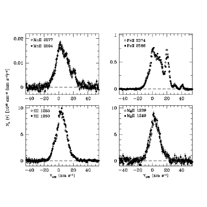
Figure 9: Representative plots of the $N_{a}(v)$ profiles for the ions Mn II, Fe II, S II, and Mg II. For most of the absorbing components, these profiles exhibit little in the way of unresolved saturated structure. The $N_{a}(v)$ profiles of Fe II are discrepant near $v_{\rm LSR}\approx+20$ km s^-1 (component 2), suggesting the presence of unresolved saturation in these transitions.

Examples of $N_{a}(v)$ profiles for the (presumably) non-depleted species S II, the moderately-depleted Mg II and Mn II, and the highly-depleted Fe II, are shown in Figure 9. For each of these ionic species two transitions with different oscillator strengths are plotted. One can see that the examples we have chosen, in general, show good agreement between the two transitions. An example where our profiles exhibit unresolved saturated structure is seen in the Fe II profiles. The $N_{a}(v)$ values near $v_{\rm LSR}\approx+21$ km s^-1 are lower in the stronger $\lambda$2586 line than the weaker $\lambda$2374 line. This is evidence for unresolved saturated structure in component 2 within these Fe II lines. For Fe II, however, it is still possible to accurately derive $N(v)$ with transitions weaker than the $\lambda$2586 transition.

Table 4 contains the velocity-integrated apparent column densities (Savage & Sembach 1991) and estimated errors for the transitions studied in this work. The sources of errors for these integrations were taken to be the same as those described above for deriving the integrated equivalent widths. We have not included the uncertainties in the $f$-values in this error budget. In the absence of unresolved saturated structure, these column densities are equivalent to the true column densities in the velocity ranges outlined in Table 1. The column densities are representative of the individual components considered here if there exists no significant blending between the components.

3.3.2 Component Fitting

The column densities derived through the $N_{a}(v)$ method above may be subject to large uncertainties in cases where the individual absorbing regions overlap significantly in velocity. In particular component 2 may be heavily contaminated by overlap with absorption due to component 1 in lightly depleted species (cf., Figure 1). To more cleanly separate the higher velocity gas seen in components 2, 3, 4, and 5 we use component fitting techniques to derive the interstellar column densities.

The component fitting approach begins with a model of the interstellar absorption spectrum, which consists of $k$ individual components described by their central velocities, $v_{k}$, Doppler spread parameters, $b_{k}$, and column densities, $N_{k}$. The individual model components are assumed to be well approximated by a Voigt profile. This model is then convolved with an appropriate instrumental line spread function (LSF), and the value of $\chi^{2}$ minimized between this blurred model and the observed line profile to determine the best-fit parameters. Our component fitting analysis makes use of software kindly provided by E. Fitzpatrick (1998, priv. comm.) and described in Spitzer & Fitzpatrick (1993) and Fitzpatrick & Spitzer (1997).

Where they exist, we have used observations taken through the SSA of the GHRS in our component fitting analysis. While these data often have lower signal to noise, the LSF of the SSA has been carefully studied by Spitzer & Fitzpatrick (1993) and has a slightly better resolution than the LSF of the LSA. However, most of the data presented here were taken through the GHRS LSA. The LSF for the GHRS LSA has not been well characterized. Robinson et al. (1998) present a LSF for the post-COSTAR LSA; however, we found this LSF inadequately matched the results derived from our fitting of SSA profiles and was not able to fit narrow deep lines correctly (e.g., component 4). In Appendix B we derive a new LSF for the post-COSTAR GHRS LSA. The new LSF is a sum of a strong narrow Gaussian and a weak broad Gaussian. The narrow component has a FWHM of 1.09 diodes, while the weak component has a FWHM of $\sim 4.21$ diodes with a peak approximately 4.5% that of the narrow component at $\lambda$2800. Therefore the broad weak component contains 15.1% of the spread function area. This fraction is a function of wavelength, however. We discuss this LSF in more detail in Appendix B.

The best fit $b$-values and column densities from our component fitting analysis are given in Table 5. The best fit central velocities are given in Table 6. We fit the blend making up component 1 with three components having approximate central velocities $\langle v_{\rm LSR}\rangle\approx-8$, 1, and 7 km s^-1, though there is some variation in the best fit values. Due to the lack of uniqueness in this central blend, we do not report here the results for these individual components, but only the sum of their column densities in Table 5. Our purpose in fitting component 1 was not to disentangle this blend, but to approximately account for the overlap of this region with the more distinct component 2.

Where several lines exist for a given ionic species, we have fit all of the profiles simultaneously. For several species it was necessary to adopt $b$-values derived from fits to other ions. This approximation was necessary when either the signal-to-noise ratio of the spectra were not high enough for the fitting to be reliable (e.g., Cr II or Ni II) or when the profiles of the components were not distinct enough to provide appropriate information to constrain the fit (e.g,. for component 2 in P II and Zn II). In these cases we have adopted relatively well-constrained $b$-values from lines of similar atomic mass. To assess the error contribution of the adopted $b$-values to our derived column densities, we have also calculated the best fit models for $b\pm 1\sigma$. The differences between the $b\pm 1\sigma$ results and the best fit $b$-value results were added in quadrature to the formal fitting error. For the S II profile we have fixed the central velocity of component 2 to that derived for Si II. This was done because the unconstrained fit yielded velocity structure and relative column densities in the central blend that were significantly different than that of any other ion, and these differences impacted the fitted component 2 parameters. We found, however, that by holding the velocity of this component we were able to obtain a fit in good agreement with our results for the other ions.

In general the component fitting results for component 1 agree with the $N_{a}(v)$ integrations, suggesting little in the way of unresolved saturated structure or confusion from component overlap. We find the column densities derived for component 2 in lightly depleted species are typically $\sim 0.2$ dex lower than the results derived from integrating the $N_{a}(v)$ profiles. This is a result of the overlap from wings of components in the low-velocity blend that are included in the $N_{a}(v)$ integration. We see that component 4 may be significantly saturated in a number of profiles by comparing the component fitting results with the column densities derived from a straight integration of the $N_{a}(v)$ profiles (e.g., Mg II and O I). The $b$-values derived from our component fitting analysis are $b\leq 2.4$ km s^-1 (FWHM$\,\lesssim 4.0$ km s^-1). Thus it is important to use the component fitting results for this cloud.

3.4 Adopted Column Densities

To derive the best column densities for component 1, we take the weighted average of all the transitions for a given species that show no evidence for unresolved saturated structure in their $N_{a}(v)$ profiles. We present our adopted final column densities in Table 7, noting where we have chosen not to use an observed transition in deriving these column densities. We are relatively certain that the column densities in Table 7 for the low-velocity absorbing components toward $\mu$ Col are not significantly affected by saturation effects. The individual clouds making up the blend of component 1 are relatively broad, and the absorption profile seems to be fully resolved by the echelle-mode resolution of 3.5 km s^-1.

In a few cases we have chosen to use the component fitting results for component 1. These cases have been marked in Table 7 and include Ni II, Fe II, and Zn II. The Zn II observations show a systematic offset of 0.08 dex between the integrated column densities of the two transitions. This cannot be due to saturation effects since the stronger of the two lines gives a higher apparent column density, exactly the opposite of the expected behavior in the presence of saturation. This behavior may be caused by uncertainties in the oscillator strengths of the transitions. We have chosen to adopt the component fitting results for Zn II because we believe the column densities are a better compromise between the two profiles than the $N_{a}(v)$ values and the formal errors are more representative of the true errors.

The final adopted column densities for components $2-5$ are from our component fitting results. Most of the values given in Table 7 are the result of simultaneously fitting all the available transitions of a given species, with exceptions noted in the table. Table 7 also includes our derivation of the H I column density along this sightline, which is described in Appendix A.

4 ABUNDANCES IN THE LOW VELOCITY GAS

In this section we discuss the observed abundances in the low-velocity absorbing regions (components 1 and 2) along the line of sight to $\mu$ Col and the implications of these abundances for interstellar dust. This velocity range (from $v_{\rm LSR}\approx-17$ to $+29$ km s^-1) not only contains the vast majority of the warm neutral absorbing column but also material associated with ionized gas along the path to $\mu$ Col. It is necessary to examine the degree to which material in primarily ionized gas may affect the derivation of relative abundances in the neutral material along this sightline. We discuss this contamination and our assessment of it in §4.1.

Throughout this paper we will be discussing the normalized gas-phase abundance of elemental species. We define the normalized gas-phase elemental abundance of a species $X$ relative to $Y$ as a function of velocity to be

$$[X/Y]_{v}\equiv\log\{N_{a}(v)_{X}/N_{a}(v)_{Y}\}-\log\{X/Y\}_{\odot},$$ (2)

where $N_{a}(v)$_X and $N_{a}(v)$_Y are the apparent column density per unit velocity for the elements $X$ and $Y$, respectively, and the quantity $\{X/Y\}_{\odot}$ is the solar or cosmic reference abundance ratio of the two species $X$ and $Y$ (e.g., the meteoritic abundances from Anders & Grevesse 1989). We will use $[X/Y]$ to denote the equivalent of Equation (2) when one uses velocity-integrated total column densities in place of $N_{a}(v)$_X and $N_{a}(v)$_Y. This nomenclature is equivalent to others’ definition of the logarithmic depletion, $D(X)$ (e.g., SSC; Spitzer & Fitzpatrick 1993). When deriving gas-phase abundances it is typically assumed $[X^{+}/Y^{+}]\approx[X/Y]$, if $X^{+}$ and $Y^{+}$ are the dominant stages of ionization in the warm neutral medium. For the most part this assumption is justified, though the effects of ionized gas along the line of sight may modify the ions in a different manner, causing this assumption to break down. We will show in §4.1 that this is not a significant effect for component 1. However, for components $3-5$ this assumption will not be appropriate (see §5).

4.1 Ionization Effects

The presence of absorption due to the ions S III, Si III, Si IV, Al III, and Fe III in our GHRS spectra and the Copernicus observations of N II strongly suggest the presence of ionized hydrogen (H⁺) along the line of sight to $\mu$ Col. The WHAM observations of this region imply the presence of ionized gas in this direction at velocities compatable with those of the ionized tracers observed by GHRS, though much of the emission may come from beyond the star. For regions primarily containing H^o, an element $X$ whose first ionization potential falls below that of hydrogen is predominantly found in its singly ionized form, $X^{+}$. Thus measurements of $X^{+}/{\rm H^{o}}$ or $X^{+}/Y^{+}$ are generally good indicators of the gas-phase abundance of the element $X$ in the neutral material. However, the inferred presence of H⁺ along the sightline to $\mu$ Col complicates this simple picture since the relative contributions of $X^{+}$ and $X^{+2}$ may be different for each element in the H⁺-containing region and will be dependent upon the ionization structure of the region. Therefore, it is important to investigate the effects of H⁺-containing regions along the line of sight on our derived gas-phase abundances.

$\mu$ Col is an O9.5 V star with $T_{eff}\approx 33,000$ K (Howarth & Prinja 1989) and is therefore hot enough to ionize its immediate surroundings. A SIMBAD search of the area within 5^∘ of $\mu$ Col reveals two B2.5 IV stars along the sightline to $\mu$ Col: $\gamma$ Col and HD 41534. These stars, with $T_{eff}\sim 20,000$ K, lie $\gtrsim$20 pc from the sightline to the star and should contribute very little to the ionized column along the sightline compared with $\mu$ Col itself. Within 10^∘ of the star there are a total of seven B stars of types B2.5 or later. Given the lack of any O-type stars within 300 pc of the $\mu$ Col sightline (SY) and the late spectral types of the B-type stars found near the sightline, we will continue under the assumption that the majority of the warm ionized gas that occurs along this sightline is contained in a photoionized nebula around $\mu$ Col. The column of H II along the line of sight can be predicted using

$$N({\rm H}^{+}) = N({\rm H^{o}}+{\rm H}^{+})-N({\rm H^{o}})$$

$$\approx N({\rm S}^{+})\cdot\{{\rm H/S}\}_{\odot}-N({\rm H^{o}}).$$

Using this approach SY predict log $N({\rm H}^{+})=19.94$. Using our accurate determination of $N({\rm H\;\mbox{\small\rm I}})$ towards $\mu$ Col (Appendix A), coupled with our high-quality S⁺ measurements, we predict $\log N({\rm H}^{+})=19.17\pm 0.14$. This estimate relies on the key assumption that the total sulfur to hydrogen abundance along this sightline is solar. The WHAM spectra and the GHRS observations of S III, Al III and Si II^∗ (see below) suggest that ionized gas contamination is most significant for component 1.

To more reliably assess the contribution of material associated with an ionized nebula about $\mu$ Col to our absorption line measurements, we have used the photoionization equilibrium code CLOUDY (v90.04; Ferland 1996, Ferland et al. 1998) to model the ionization and temperature structure of such an H II region. To estimate the stellar spectrum from $\mu$ Col for use in our photoionization models, we adopt an ATLAS line-blanketed model atmosphere (Kurucz 1991) with the stellar parameters $T_{eff}=33,000$, $\log(g)=4.0$ and $L_{*}=2.6\times 10^{4}\ L_{\odot}\ =1\times 10^{38}$ ergs s^-1, close to the values estimated by Howarth & Prinja (1989) for $\mu$ Col. For a range of densities and filling factors of the ambient ISM, we have calculated the ionization and temperature structure of model nebulae from a distance 0.03 pc from the star to the point where the electron density, $n_{e}$, falls to $5\%$ of the total hydrogen density, $n_{\rm H}$. We have used solar abundances throughout. The ambient densities used in the models presented here are $n_{\rm H}=0.02,0.05$, 0.2, and 0.5 cm^-3. The densities 0.05 and 0.2 cm^-3 are approximately the average line of sight density, and the estimated density of the H II region gas from the excited states of N II (SY) and Si II (see §4.4). The highest value was used to study regions more dense than the limit of $n_{e}\gtrsim 0.2$ cm^-3, while the lowest is used to show the relative constancy of the results. The first three models are those presented in Brandt et al. (1999) to discuss the source of the Si IV absorption along the line of sight to $\mu$ Col. Similar models have also been presented by Howk & Savage (1999) to derive the gas-phase abundance of [Al/S] in the ionized medium of the Galaxy.

In order to match the observational constraints, we assume all of the column density of S III arises in the photoionized region about the star. For the densities considered, we vary the volume filling factor of the material until a match to the observed S III column density of $\log N(\mbox{{S~{}III}})=13.82$ is obtained. Table 8 contains the physical parameters for each of our models and the predicted column densities of important ionic species. The predicted column densities of H⁺ for the models given in Table 8 are in the range $\log N(\mbox{H$\;${\small\rm II}})=19.01-19.10$, which is in rough agreement with the H II column density predicted by scaling our S II column density according to Equation (4.1). The H II column densities from our CLOUDY models are mildly sensitive to where the model nebulae are truncated.

Among the most important conclusions we have drawn from our modelling of the $\mu$ Col H II region is that the ratio of $N({\rm Al}^{+2})/N({\rm S}^{+2})$ predicted to occur in an H II region is relatively insensitive to the model assumptions. Howk & Savage (1999) have used similar models and observed values of $N({\rm Al}^{+2})$ and $N({\rm S}^{+2})$ to determine the normalized gas-phase abundance of Al to S in the H II region surrounding $\mu$ Col. Their model-corrected result,

$$[{\rm Al/S}]_{{\rm H\,II}}=-0.78\pm 0.08,$$

is insensitive to the adopted density or filling factor of the nebula, and the ionizing photon flux of the star. Further, the sensitivity to the shape of the ionizing spectrum (i.e., to $T_{eff}$), is also relatively small. The error estimate comes from the standard deviation about the mean predicted value of $N({\rm Al}^{+2})/N({\rm S}^{+2})$ for models using input spectra in the range $27,000\leq T_{eff}\leq 39,000$ K (see Howk & Savage 1999).

A similar calculation can be made regarding the gas-phase abundance of Fe relative to S in the H II region about $\mu$ Col. Howk & Savage (1999) have shown that values of $N({\rm Fe}^{+2})/N({\rm S}^{+2})$ predicted by the models are much more sensitive to uncertainties in the input effective temperature of the ionizing source. Using observations of $N({\rm Fe}^{+2})$ and $N({\rm S}^{+2})$ and CLOUDY models, they determine

$$[{\rm Fe/S}]_{{\rm H\,II}}=-0.87\pm 0.21$$

in the $\mu$ Col H II region.

The sub-solar abundances of Al and Fe in the $\mu$ Col H II region likely implies the existence of dust in the ionized ISM about this star. An Al depletion of 0.8 dex is similar to that found for refractory elements along warm disk+halo sightlines (Sembach & Savage 1996). The similar depletion of Fe is also consistent with warm disk+halo sightlines.

For the undepleted ions S II and P II, which are the dominant ionization stages in the WNM, our models predict absorption from material in the H II region may account for $\sim 10$% of the total observed absorbing column density. Thus the presence of a low-density H II region surrounding $\mu$ Col may add a systematic contribution of $\approx 0.04$ to 0.05 dex to the column densities of undepleted species in component 1. This is a relatively small contribution. We have chosen not to report the photoionization model results for the undepleted species Zn II given the large uncertainties in the adopted atomic parameters, particularly the recombination coefficients and ionization cross sections, for this element.

Assessing the impact of the H II region to the measurements of highly depleted species is more complicated. We have assumed solar abundances for our model H II region. Given our analysis of the Al III and Fe III absorption above, using solar abundance models will over-estimate the contribution of the H II region to the total line of sight absorption measurements for depleted species. This can easily be seen in the results tabulated for Fe II in Table 8. In some cases we predict more Fe II absorption than is actually measured for component 1. Because there is evidence for sub-solar abundances in the measured ratios $N({\rm Fe}^{+2})/N({\rm S}^{+2})$ and $N({\rm Al}^{+2})/N({\rm S}^{+2})$, we have confidence that dust exists in the ionized gas about $\mu$ Col.

The estimated abundance [Fe/S] in the H II region is roughly consistent with that of warm disk+halo sightlines. We can use this abundance to estimate the corresponding abundances of the elements Mg, Si, and Mn in the H II region. The compiled logarithmic depletions (equivalent to our normalized gas-phase abundances) of these elements are tabulated in Savage & Sembach (1996) for such sightlines to be

$$[{\rm Mg/H}]\approx-0.31;\ [{\rm Si/H}]\approx-0.25;\ {\rm and}\ [{\rm Mn/H}]\approx-0.66,$$

where we have corrected the value of [Mg/H] for our adopted $f$-values. If we apply these depletions to our model H II region results, the relative contribution of H II region gas to the measured total column densities of these species is approximately

$$\mbox{{Mg~{}II}}:0.05\ {\rm dex};\ \mbox{{Si~{}II}}:0.06\ {\rm dex};\ \mbox{{Mn~{}II}}:0.09\ {\rm dex};\ {\rm and}\ \mbox{{Fe~{}II}}:0.06\ {\rm dex},$$

where we have assumed [Fe/H]$=-0.87$. Thus, material associated with the H II region may provide a relatively small, though not insignificant, contribution (uncertainty) to the measured column densities. This contribution is not large enough to hinder our major conclusions regarding the gas-phase abundances of the primarily neutral medium. We will assume that the contribution of H II region gas to the measurements of Zn II is similar to that of the undepleted elements S II and P II. For Cr II and Ni II we find results similar to those of Fe II and Mn II, respectively. It is important to point out that the expected contribution of an ionized nebula to the depleted and non-depleted species are very similar. Thus while the contributions to the S II and Fe II column densities from the ionized nebula are of order 0.05 to 0.06 dex, the ratio $N(\mbox{Fe$\;${\small\rm II}})/N(\mbox{S$\;${\small\rm II}})$ is only changed by $\sim 0.01$ dex. However, when comparing singly-ionized species to neutral hydrogen, this contribution is more significant.

The aforementioned uncertainties in the fundamental stellar parameters (temperature, luminosity, and surface gravity) do not seriously affect our estimates of contamination from gas in an H II region around $\mu$ Col. The temperature and surface gravity of the star change the shape of the spectrum, but over the range of allowable values, we have found varying these parameters changes little in our models. Changing the luminosity does not affect the results at all. In this case the important parameter is the “ionization parameter” (see Howk & Savage 1999), which can be made made constant with varying luminosity by simply adjusting the ambient density and/or filling factor.

It is important to constrain the ionization fraction of the primarily neutral gas along the sightline. There may be partially ionized gas in the H I-containing regions along the sightline that do not contribute to the S III used to constrain our H II region models, but which may contribute (particularly) to the S II column density along this sightline. We can roughly estimate the ionization fraction $x_{e}\equiv n_{e}/n_{\rm H}$ of the neutral regions using the Ar I measurements of SY with the work of Sofia & Jenkins (1998; hereafter SJ). Sofia & Jenkins have suggested that the intrinsic Ar/H abundance in the ISM is close to to the solar system abundance [following SJ we adopt $12.0+\log({\rm Ar/H})_{\odot}=6.52$], and that sub-solar Ar I/H I measurements reflect the over-ionization of Ar I relative to H I. This over-ionization of Ar I is a result of its very large ionization cross section relative to that of H I. Sofia & Jenkins develop a formalism to relate the observed discrepancy, $[{\rm Ar/H}]$, between the observed and expected Ar abundance to the ionization fraction, $x_{e}$, along an interstellar sightline (see their Equation 11). Their treatment incorporates the relevant ionization and recombination rates, effects of charge exchange reactions, and photoionization into high ionization states of Ar through a quantity they denote $P\arcmin_{\rm Ar}$. Characteristic values of $P\arcmin_{\rm Ar}$ for various interstellar conditions and ionizing spectra are tabulated in their Table 4. Using the Ar I measurements of SY, corrected for the suggested Ar I oscillator strengths used in SJ, we find $[{\rm Ar/H}]=-0.24\pm 0.10$ towards $\mu$ Col using our $N(\mbox{H$\;${\small\rm I}})$ measurement. Thus it would seem that some degree of ionization is present even in the neutral gas along this sightline, unless the reference abundance of Ar is incorrect. Using Equation (11) from SJ, with an estimate of $P\arcmin_{\rm Ar}=10\pm 5$ from their Table 4, we find $x_{e}=0.09\pm 0.07$. Therefore we expect the contribution of ionized hydrogen to the total neutral column density due to partially-ionized gas to be $0.037\pm 0.028$ dex. Thus there could be an additional correction of $\sim-0.04$ dex needed to account for partially-ionized gas in the H I regions along the $\mu$ Col sightline.

We note that the relative abundance [Ar/S] derived with Ar I and S II measurements is extremely sensitive to relatively small amounts of ionized gas along a given sightline since the measured gas phase S II and Ar I increase and decrease, respectively, as the level of ionization increases. Furthermore, neither of these elements is expected to be incorporated into dust grains in large amounts (see SJ), and their nucleosynthetic origins are the same, both being $\alpha$-process elements primarily produced in high-mass stars. The usefulness of [Ar/H] measurements for identifying the existence of partially-ionized gas has been emphasized by SJ; we suggest that the [Ar/S] ratio, which can be determined as a function of velocity, is an even more sensitive indicator of the combined effects of partially-ionized gas in H I-bearing regions and H II region contamination.

4.2 Gas-Phase Abundances

Table 9 contains the values of $[X/{\rm S}]$ in the low-velocity components 1 and 2 for the elements considered here. For comparison with other sightlines and QSO absorption line systems we also give the sightline integrated values of [$X$/H] for each element $X$. These results are derived from the adopted column densities presented in Table 7. Also given in this table is the adopted solar reference abundance for each element relative to hydrogen, and the normalized gas-phase abundances for components 3 and 4, which will be discussed in §5. The quoted errors here contain only those described in §3.2. Our adopted solar reference abundance system is taken from Savage & Sembach (1996a), who rely primarily on the meteoritic abundances of Anders & Grevesse (1989) with updates for C, N, and O by Grevesse & Noels (1993).

We have plotted the data from Table 9 in Figure 10. The ordinate of these plots is the gas-phase abundance for the elements listed along the abscissa, normalized to S. The top panel of Figure 10 contains only the data from components 1 and 2. The bottom panel also shows these data, but we have overlayed the values $[X/{\rm S}]$ for the warm cloud along the $\zeta$ Oph sightline (cloud A of Savage et al. 1992) as the dashed line, and for the spread of warm halo cloud abundances from Sembach & Savage (1996) as the hatched region. Data for the gas-phase abundances of interstellar Ti in individual halo clouds are sparse. For Ti we plot an upper limit equal to that of Ni and a lower limit that is equal to the lower limit of Fe in these clouds. The values of $[X/{\rm S}]$ from Savage et al. (1992) and Sembach & Savage (1996) have been adjusted to reflect our choice of oscillator strengths.

The values of $[X/{\rm S}]$ for elements in the component 1 blend are quite similar to those found in the warm $\zeta$ Oph cloud. This was also the conclusion of SSC, though with considerably more uncertainty. This level of sub-solar abundances is consistent with other “warm disk”-like clouds as categorized by Sembach & Savage (1996). Similarly, the relative abundance pattern seen for component 2 is mostly within the small range of “halo” cloud values. This is somewhat deceiving, however, since the earlier GHRS data for the $\mu$ Col sightline (SSC) were used by Sembach & Sembach (1996) in defining this spread of values. The new data presented here for component 2 support the claim of Sembach & Savage that the upper-limit of $[X/{\rm S}]$ for many elements shows relatively little cloud-to-cloud variation about the mean for each species. What is perhaps surprising, given the new distance to $\mu$ Col, is that a cloud within $\approx 400$ pc of the sun ($z\lesssim 180$ pc) has abundance patterns similar to clouds at relatively large heights from the plane. If one adopts the distance derived from the Vacca et al. (1996) absolute magnitude scale, namely $d\sim 790$ pc, the $z$-height becomes $z\sim 360$ pc from the midplane. This is more than one H I scale height above the midplane.

In the gas of component 1, the values [Si/S] and [Mg/S] are slightly higher than those seen along the $\zeta$ Oph sightline warm cloud. Using the oscillator strengths suggested by Fitzpatrick (1997), Si and Mg show quite similar abundance patterns. Given the similarity of the Si II $\lambda$1808 line profile to those of Mg II $\lambda\lambda$1239, 1240, this is not a surprising result. The similar abundance behavior of these elements is seen even more clearly in plots of $[X/{\rm S}]_{v}$, the gas-phase abundance of an element $X$ as a function of velocity.

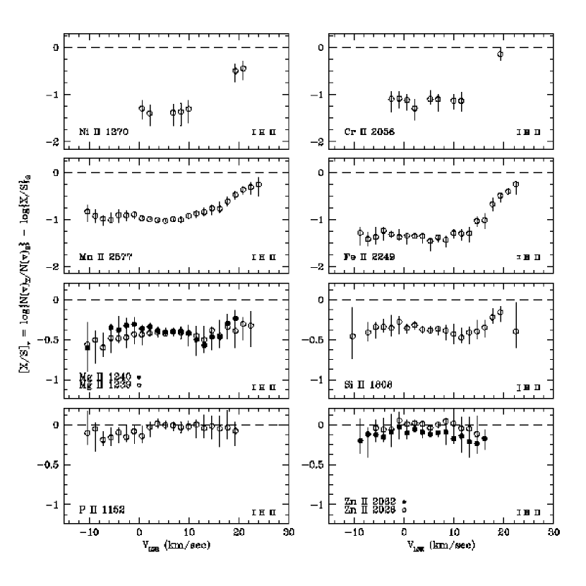
Figure 11: Normalized gas-phase abundances of several ionic species relative to S as a function of velocity. Plotted are the ratios of P II, Zn II, Mg II, Si II, Mn II, Fe II, Ni II, and Cr II to S II, normalized to the solar system meteoritic abundances of Anders & Grevesse (1989), as a function of velocity. The error bars represent $1\sigma$ uncertanties from photon statistics, continuum fits, and zero point uncertainties as well as a contribution for velocity shifts between the profiles. In the lower right of each panel is a bar representing the estimated size of the uncertainty due to contamination from material in an H II region surrounding $\mu$ Col. For Zn II and Mg II we have plotted both transitions since there are slight differences between them.

Figure 11 presents plots of the normalized gas-phase abundances for several elements as a function of velocity, using the adopted solar system abundances listed in Table 9 (principally the meteoritic abundances of Anders & Grevesse 1989). We have plotted the ratios of P II, Zn II, Mg II, Si II, Mn II, Fe II, Ni II, and Cr II to S II in this figure. For all of the species but Ni II, the width of the data bins is half a resolution element (i.e., $\approx 1.75$ km s^-1 or two of the original data points for profiles taken with four substeps per diode). We have binned the Ni II profile to one point per resolution element. The error bars represent the sources of errors discussed in §3.2 as well as a contribution from possible velocity scale offsets. The latter was derived by shifting one profile relative to the other by half a resolution element (in both the positive and negative velocity directions) and adding the resulting errors in quadrature to those of §3.2. These velocity shift error estimates are the primary cause of the asymmetric error bars in Figure 11. The range over which data points are plotted in this figure is determined by the significance of each point once we have added all of the sources of noise. This presentation assumes that the $N_{a}(v)\approx N(v)$ and $[X^{+}/{\rm S}^{+}]_{v}\approx[X/{\rm S}]_{v}$. The former of these assumptions is justified by our examination of the $N_{a}(v)$ profiles of each of the ions for which unresolved saturation might be present. In no case do we find evidence for saturation effects in the transitions presented in Figure 11. The latter of these assumptions is likely valid for material in the warm neutral medium. In the lower-right of each panel we have included a bar representing the maximum degree of uncertainty the $\mu$ Col H II region is thought to add to the individual measurements, as discussed in the previous subsection.

There is an increase in the gas-phase abundances of the elements Fe, Mn, Cr, Ni and possibly Si near $v_{\rm LSR}\approx+20$ km s^-1, which is associated with the significant strengthening of component 2 in moderately- and heavily-depleted species. However, one of the more striking aspects of Figure 11 is the relative constancy of the ratios plotted here over the range $-10\lesssim v_{\rm LSR}\lesssim+14$ km s^-1. The absorbing clouds making up the component 1 blend have similar gas-phase abundances. The $[X/{\rm S}]_{v}$ profiles for Si and Mg are quite similar, with $[{\rm Si/S}]_{v}\approx[{\rm Mg/S}]_{v}\approx-0.4$ dex. The Mg abundance profile is slightly flatter than the Si profile. Figures 10 and 11 show that Mg and Si trace each other well (see Fitzpatrick 1997).

The abundances $[X/{\rm S}]_{v}$ for the elements P and Zn are consistent with solar system abundances, i.e., [P/S]${}_{v}\approx$ [Zn/S]_v $\approx$ 0. This behavior holds over the whole velocity range considered in Figure 11. This supports our choice of solar system abundances as a reference for this dataset. B stars in the solar neighborhood may have lower intrinsic abundances than the sun (e.g., Kilian-Montenbruck et al. 1994; Gies & Lambert 1992), suggesting the proper “cosmic” reference abundance may be sub-solar by $\sim 0.2$ dex. In the case of the sightline towards $\mu$ Col, we observe gas with solar system abundance ratios of P and Zn to S, which we believe argues for using solar system reference abundances for these clouds. The choice of solar relative abundances for these clouds is particularly strong given the sources of metal production for S, an $\alpha$-element, are thought to be different stars than those producing Zn, which traces Fe-peak elements. Given these elemental abundance ratios, we will rely primarily upon the solar system abundances of Anders & Grevesse (1989) as a cosmic reference (as compiled in Savage & Sembach 1996a).

4.3 Implications for Interstellar Dust

The sub-solar gas-phase abundance patterns seen in Figures 10 and 11 likely represent the imprint of elemental incorporation into interstellar dust grains. Our arguments from §4.1 suggest that the ionized gas contribution to the measured total column of each of the species considered in Figures 10 and 11 is minor, certainly less than $\sim 0.1$ dex. The depletion of elements from the gas- to the solid-phase is a well known phenomenon and allows us to infer the elemental make-up of dust grains in the diffuse ISM (Savage & Sembach 1996a).

The striking similarities between the normalized abundances in the warm $\zeta$ Oph cloud and the material making up component 1 along the $\mu$ Col sightline suggest that this level of depletion, or incorporation of elements into the dust-phase, is relatively common among low H I column density clouds that make up the warm neutral medium in the solar neighborhood (SSC). The H I column densities of these two cloud complexes are quite similar [$\log N(\mbox{H$\;${\small\rm I}})_{\zeta\ {\rm Oph\ A}}\approx 19.74$; Savage et al. 1992].

Of interest for determining the types of grains present in the ISM is the dust-phase abundance of each element with respect to hydrogen. The dust-phase abundance of a species $X$ relative to hydrogen, $(X/{\rm H})_{d}$, is given by

$$(X/{\rm H})_{d}=(X/{\rm H})_{c}-(X/{\rm H})_{g},$$ (4)

where the subscripts $d,\ c,$ and $g$ refer to the dust-phase, cosmic, and gas-phase abundances of $X$, respectively. Table 10 gives the dust-phase abundances of a series of elements relative to H (given in parts per million H) and relative to Si for components 1 and 2. We also give the dust-phase abundances of Mg, Si, and Fe when adopting B-star abundances as determined by Gies & Lambert (1992) and Kilian-Montenbruck et al. (1994). Gies & Lambert do not derive the abundance of Mg in their work, so we have adopted the Mg abundance from Kilian-Montenbruck et al. in this case. The values of $(X/{\rm H})_{c}$ are given for each element in the different reference systems. The values $(X/{\rm H})_{d}$ have been derived assuming S is present in its cosmic abundance, i.e., is not depleted into grains. The cosmic sulfur abundances in the three systems are: (S/H)${}_{c}=1.9\times 10^{-5}$ (Anders & Grevesse 1989); (S/H)${}_{c}=1.6\times 10^{-5}$ (Gies & Lambert 1992); and (S/H)${}_{c}=9.3\times 10^{-6}$ (Kilian-Montenbruck et al. 1994). We have not included P or Zn in this table, as neither shows any evidence for incorporation into dust grains in our data.

Among the elements considered here, the most abundant in dust grains are Mg, Si, and Fe. The solid forms of these elements in the ISM are thought to include silicates, oxides and possibly metallic iron. Among the silicate forms thought to be most common are various pyroxenes, (Mg, Fe)SiO₃, and olivines, (Mg, Fe)₂SiO₄ (Ossenkopf et al. 1992). If the Mg- and Fe-bearing dust in the ISM towards $\mu$ Col were primarily made up of only these types of silicates, one would expect a ratio of [(Fe+Mg)/Si]${}_{d}\approx 1-2$. Assuming the solar abundances given in Table 10, we find:

$$\left[{\rm(Fe+Mg)}/{\rm Si}\right]_{d} = 2.70\pm 0.11\quad\mbox{in component 1; and}$$

$$\left[{\rm(Fe+Mg)}/{\rm Si}\right]_{d} = \phantom{0}3.3\pm 1.4\phantom{0}\quad\mbox{in component 2.}$$

If one adopts the Kilian-Montenbruck et al. (1994) B-star abundances as the cosmic reference, these values become: $[{\rm(Fe+Mg)}/{\rm Si}]_{d}=5.06\pm 0.24$ in component 1; and $[{\rm(Fe+Mg)}/{\rm Si}]_{d}=15\pm 14$ in component 2. The abundances of Gies & Lambert (1992) yield intermediate values. The composition of dust grains containing Mg, Si, and Fe in the material making up component 1 is inconsistent with the sole consituent of this dust being silicate pyroxenes or olivines, irrespective of the cosmic abundance one chooses to adopt. Component 2 may be similar in this regard, but the large uncertainties make this statement much less certain.

Whittet et al. (1997) have recently reported on the detection of O$-$H stretching modes in OH groups along the diffuse sightline to Cygnus OB2 No. 12 (VI Cygni No. 12) using the Infrared Space Observatory. Given the lack of ices along this sightline, they attribute this feature to hydrated silicates. The values of (Mg/Si)_d in components 1 and 2, assuming solar system abundances, is consistent with the incorporation of Mg into a mixture of the phyllosilicates talc, Mg₃Si₄O₁₀[OH]₂, and serpentine, Mg₃Si₂O₅[OH]₄. However, Whittet et al. find a very small fraction of silicates along that sightline are hydrated. Thus we believe it unlikely phyllosilicates can provide for enough of the Mg to allow Fe-bearing silicates to account for the total dust-phase Fe abundance. Some amount of the Mg- and Fe-bearing dust is therefore likely in the form of oxides or pure iron grains. Examples of Mg-, and Fe-bearing oxides include MgO, FeO, Fe₂O₃, and Fe₃O₄ (Nuth & Hecht 1990; Fadeyev 1988).

It is clear from Figures 10 and 11 that there is a larger gas-phase abundance of the refractory elements in component 2 than in component 1. In particular, the gas-phase abundances of Fe, Cr, and Ni show much higher abundances in Figure 10. In principle higher gas-phase abundances of Fe-peak elements in interstellar clouds could be interpreted as evidence for enrichment by Type Ia SNe (Jenkins & Wallerstein 1996). We discount this mechanism for providing the enhanced gas-phase abundances seen in component 2 over component 1 along the $\mu$ Col sightline, suggesting instead that the large enhancements seen in the Fe-peak elements over the other elements in Figure 10 are a result of the return to the gas phase of highly depleted elements. The increases in the gas-phase abundances per million H in component 2 over component 1 are: $15.4\pm 1.1$ for Fe, $11\pm 4$ for Si, $0.018\pm 0.006$ for Ti, $0.27\pm 0.04$ for Cr, $0.078\pm 0.015$ for Mn, and $0.54\pm 0.07$ for Ni. If we were to assume gas with abundances similar to component 1 had been enriched by gas from a Type Ia SN, we would expect factors of 2.5 and $3-7$ more Mn and Ni, respectively, relative to Fe using the nucleosynthetic yields of Nomoto et al. (1984) and Thielemann et al. (1986). Also, relative to the models of Type Ia SN nucleosynthesis, the observed increase in Si relative to Fe is a factor of $\sim 2$ too large, while the increase in Ti to Fe is too high by a factor of 2.5 to 160, depending upon the exact nucleosynthesis result used. Therefore, we conclude that the increase in gas-phase abundances observed in component 2 relative to component 1 is likely not due to enrichment by the nucleosynthetic products of a Type Ia SN.

We interpret the higher gas-phase abundances seen in component 2 as a return of elements to the gas phase from the solid phase in material that has been processed by a shock(s). The dust-phase abundances of many elements in component 2 have been lowered relative to those in component 1. Examining the data in Table 10 we see that relative to component 1, the dust-phase abundances of Si, Mg, and Fe have changed by approximately a factor of two. The values of $[{\rm(Fe+Mg)}/{\rm Si}]_{d}$ in component 2 are consistent with those of component 1 given the large errors for this component. There is evidence for lower dust-phase abundances of Si, Fe, Ti, Cr, Mn, and Ni in component 2. If the dust-phase abundances of the warm $\zeta$ Oph cloud and the clouds making up component 1 are characteristic of a standard depletion in the low-density WNM of the Galaxy, we can estimate the fraction of material returned to the gas-phase from dust in component 2. The data in Table 10 suggest the return of $(55\pm 20)\%$ of Si, $(50\pm 4)$% of Fe, $(23\pm 8)$% of Ti, $(60\pm 9)$% of Cr, $(26\pm 5)$% of Mn, and $(32\pm 4)$% of Ni to the gas phase from dust grains, when compared to the values appropriate for component 1.

If one interprets the differences in abundance patterns between components 1 and 2 as evidence for the stripping of grain mantles from standard dust-phase abundance of the WNM, the composition of the mantles may be inferred from a direct comparison of the dust-phase abundances of components 1 and 2. The data for the $\mu$ Col sightline then suggest that the mantles of dust grains are consistent with silicate and oxide components. Our large errors in the values for component 2 make a detailed determination of the mantle composition difficult.

4.4 Physical Conditions

In this subsection we discuss the information about the physical conditions in the low-velocity material towards $\mu$ Col contained in our absorption line data. The approaches used here are well-discussed in the works of Spitzer & Fitzpatrick (1993, 1995) and Fitzpatrick & Spitzer (1994, 1997).

4.4.1 Electron Densities in the Ionized Gas

Copernicus observations of N II, N II^∗, and N II^∗∗ have yielded estimates for the average electron density in the ionized gas, $\langle n_{e,i}\rangle$, along the sightline to $\mu$ Col (SY). These authors’ estimates yield $\langle n_{e,i}\rangle\sim 0.16$ to 0.22 cm^-3 for the ionized gas. We detect weak absorption arising from the excited ${}^{2}P_{3/2}$ fine structure level of Si II at $\lambda$1264.738 in our GHRS dataset. This allows us to verify the results of SY. The equation for collisional excitation equilibrium of the Si⁺ levels may be written

$$A_{21}n({\rm Si}^{+*})+\gamma_{21}n_{e}n({\rm Si}^{+})=\gamma_{12}n_{e}n({\rm Si}^{+}),$$ (5)

where $\gamma_{12}$ and $\gamma_{21}$ are the rate coefficient for collisional excitation and de-excitation, respectively, and $A_{21}$ the spontaneous downward transition probability. In the case of ion excitation by electrons we write (Spitzer 1978)

$$\gamma_{12}=\frac{8.63\times 10^{-6}}{g_{1}T^{1/2}}\Omega_{12}\exp\left(\frac{-E_{12}}{kT}\right)\ {\rm cm}^{3}\ {\rm s}^{-1}.$$ (6)

For warm gas like that expected in an H II region, exp$(E_{12}/kT)\approx 1.0$ (to the accuracies being considered here). We adopt the values $A_{21}=2.17\times 10^{-4}$ s^-1 (Mendoza 1983; his Appendix), $\Omega_{12}=5.58$ (Osterbrock 1989; his Table 3.3), and the statistical weight $g_{1}=2$. Replacing the particle densities with column densities we have

$$\langle n_{e,i}\rangle=9.0T^{1/2}\frac{N({\rm Si}^{+*})}{N({\rm Si}^{+})},$$ (7)

where we have ignored collisional de-excitation. The effects of collisional de-excitation are negligible when $n_{e}\ll n_{cr}$, where the critical density, $n_{cr}$, is given by $n_{cr}=A_{21}/\gamma_{21}$. For $T=8000$ K the critical density is $n_{cr}\approx 1600$ cm^-3.

Using the integrated column density of Si II in component 1 yields $\langle n_{e,i}\rangle=0.2$ cm^-3. This result assumes $T=8000$ K, and scales as $T^{1/2}$. This value is a lower limit to the true electron density, $n_{e,i}$. The Si⁺ absorption includes contributions from both H I and H II regions, while it is likely that the Si^+∗ absorption comes primarily from only the densest gas of H II-bearing regions. The column of Si⁺ associated with the ionized gas is overestimated, making $n_{e,i}$ too small. The results of our photoionization modelling in §4.1 suggest that the column density of Si II arising in the H II region about $\mu$ Col is likely $\log N(\mbox{{Si~{}II}})\approx 14.3$. If we adopt this value for the column density of Si II associated with the ionized gas and assume that all of the Si II^∗ arises in this H II, we can derive an upper limit for $n_{e,i}$. Combining these two limits yields

$$0.2\ {\rm cm}^{-3}\,\lesssim n_{e,i}\,\lesssim 1.2\ {\rm cm}^{-3}.$$

The upper limit is larger than the values we’ve used for modelling the $\mu$ Col H II region, but the conclusions drawn in §4.1 are not sensitive to the ambient density.

4.4.2 Electron Temperatures and Densities in the Neutral Gas

We estimate the electron temperatures and densities of the primarily neutral material in the low-velocity components 1 and 2 by examining the ionization equilibrium of Ca and Mg in these clouds. The equation for ionization equilibrium of the ionic stages $X^{i}$, $X^{i+1}$ of an element $X$ may be written

$$\Gamma(X^{i})n(X^{i})=\alpha(X^{i})n_{e}n(X^{i+1}),$$ (8)

where $\alpha(X^{i})$ is the recombination coefficient of $X^{i+1}$ to $X^{i}$ and $\Gamma(X^{i})$ the ionization rate of $X^{i}$. The value $\alpha(X^{i})$ is the sum of the radiative recombination coefficient, $\alpha_{rad}(X^{i})$, and the dielectronic recombination coefficient, $\alpha_{di}(X^{i})$, and is a function of temperature. Using Equation (8) simultaneously for Ca⁺/Ca⁺⁺ and Mg^o/Mg⁺ ionization equilibrium can yield estimates of both the electron temperatures and densities.

For the recombination coefficients we adopt the fits suggested in the compilation of atomic data by D. Verner. Namely for the Mg^o recombination coefficients we use $\alpha_{di}({\rm Mg}^{\rm o})=4.49\times 10^{-4}T^{-3/2}\exp(-5.01\times 10^{4}/T)\left[1+2.1\times 10^{-2}\exp(-2.81\times 10^{4}/T)\right]$ cm³ s^-1 and $\alpha_{rad}({\rm Mg}^{\rm o})=1.4\times 10^{-13}\left(T/10^{4}\right)^{-0.855}$ cm³ s^-1 from Shull & Van Steenberg (1982) and Aldrovandi & Péquignot (1973), respectively. We assume a photoionization rate $\Gamma({\rm Mg}^{\rm o})=4.0\times 10^{-11}$ s^-1 (Frisch et al. 1990). For Ca we adopt the values $\alpha({\rm Ca}^{+})\approx\alpha_{rad}({\rm Ca}^{+})=6.78\times 10^{-13}\left(T/10^{4}\right)^{-0.8}$ cm³ s^-1 from Shull & Van Steenberg (1982). We assume $\Gamma({\rm Ca}^{+})=2.0\times 10^{-12}$ s^-1 (Péquignot & Aldrovandi 1986). Unfortunately, we do not measure the dominant ionization stage Ca⁺⁺. To proceed we assume that the gas-phase abundances of Ca and Fe are approximately the same in the WNM towards $\mu$ Col (see Jenkins 1987). The profiles of the Ca II and Fe II (e.g., $\lambda$2249) transitions are very similar for the $\mu$ Col sightline, suggesting this is a reasonable assumption. Using this approximation we can substitute $n({\rm Fe}^{+})\cdot\{{\rm Ca/Fe}\}_{\odot}$ for $n({\rm Ca}^{++})$.

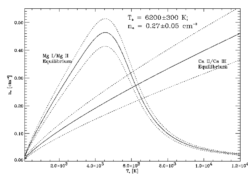
Figure 12: Plot of the predicted electron density, $n_{e}$, as a function of temperature, $T_{e}$, using Mg I/Mg II and Ca II/Ca III ionization equilibrium. The solid lines represent the trends in $n_{e}$ with $T_{e}$ for the most likely ratios of these ionization stages. The dotted lines represent the $1\sigma$ uncertainties (not including uncertainties in the atomic data). The values predicted by the intersection of the Mg I/Mg II and Ca II/Ca III curves are $\langle T_{e}\rangle=6200\pm 300$ K and $\langle n_{e}\rangle=0.27\pm 0.05$ cm^-3.

Figure 12 shows the relationship of $n_{e}$ and $T_{e}$ for Ca and Mg ionization equilibrium in component 1. The solid lines represent the dependence of $n_{e}$ on $T_{e}$ for each diagnostic given the best values of the $N({\rm Ca}^{+})/N({\rm Fe}^{+})$ and $N({\rm Mg^{o}})/N({\rm Mg}^{+})$ ratios. The dotted lines give the $1\sigma$ error limits based upon the sources of error given in §3.2. While there is a formal solution for very low temperatures, the high-temperature solution is more applicable to the gas being considered here. The results of this approach for components 1 and 2 are given in Table 1. Also shown are the electron temperatures and densities for component 4 (see below). The treatment of Equation (8) neglects the charge-exchange reactions between neutral Mg and ionized H (Allan et al. 1988), but we have found including these reactions makes little difference to the final results.

In principle one can derive the neutral hydrogen density in WNM clouds using observations of C I absorption from the ${}^{3}P_{0}$, ${}^{3}P_{1}$, and ${}^{3}P_{2}$ levels. However, our marginal detections of the first excited ${}^{3}P_{1}$ level and limits on the ${}^{3}P_{2}$ column densities allow us only to place limits on the neutral hydrogen density. We find $\log N_{10}\equiv\log N(\mbox{{C~{}I}}\ \,^{3}P_{1})-\log N(\mbox{{C~{}I}}\ \,^{3}P_{0})\lesssim-0.37$ and $\log N_{20}\equiv\log N(\mbox{{C~{}I}}\ \,^{3}P_{2})-\log N(\mbox{{C~{}I}}\ \,^{3}P_{1})\lesssim-0.56$ in component 1. Interpolating between the values given in the tabulation of Keenan (1989), and assuming $T\approx 6000$ K and $n_{e}\approx 0.3$ derived above, we estimate $n_{\rm H}<10$ cm^-3 in component 1.

5 IONIZATION AND DUST IN THE INTERMEDIATE-VELOCITY GAS

5.1 Photoionized Gas at Intermediate Positive Velocities

Components 3 and 4 along the sightline to $\mu$ Col are examples of low total column density intermediate-velocity clouds (IVCs). The hydrogen column density for component 4 is likely $\log N({\rm H})\sim 17.3-17.7$ (see below). With an absorption cross-section of $6.3\times 10^{-18}$ cm² for atomic hydrogen (Spitzer 1978), this implies an optical depth of order unity for this cloud at $\lambda$912. Thus, the assumption that the gas-phase abundances of a cloud are accurately traced by the dominant stage of ionization in the neutral medium may break down for components 3 and 4. Further, the effects of ionization will differ from species to species, depending upon that ionic species’ ionization potential and photoionization cross section, its recombination coefficient, including the effects dielectronic recombination, and the availability of charge-exchange reaction pathways.

The species for which we have well-determined column densities for component 4 include N I, O I, Mg I and II, Si II and III, Fe II, and Al II. In Figure 13 we plot the the values of [$X$/Si] for the species O, Mg, Si, Al, Mn, and Fe. The values [$X$/Si] for components 3 and 4, derived from the ratios of the usually dominant species, are also given in Table 9. The unusual nature of this component can easily be seen in Figure 13. Typically Si is moderately incorporated into grains in the diffuse ISM (e.g., in components 1 and 2), while N has only moderately sub-solar gas phase abundances in the solar neighborhood (Meyer et al. (1997) find $[{\rm N/H}]\approx-0.1$). Therefore in the WNM we expect to find $[{\rm N/Si}]>0$. In Figure 13 we see that [N/Si] derived from measurements of N I and Si II is sub-solar. At the same time we find that [Fe/Si] is almost indistinguishable from that seen in component 2 and similar to halo cloud values. We believe that the pattern of gas-phase column densities observed in component 4 is a result of photoionization of a low column density cloud with somewhat typical halo-like gas-phase abundances. The uncertainties in this ionization, however, hinder our ability to make firm conclusions regarding the gas-phase abundances of the intermediate velocity clouds towards $\mu$ Col.

For a few species we can place quite stringent limits on the true gas-phase abundances. We observe the ionization states Si II, III, and IV and therefore have a very good measure of the total column density of Si in component 4, $\log N({\rm Si})=12.85\pm 0.03$, i.e., the contributions from Si III and IV are negligible. We can place similar constraints on the abundance of Al in this material. The $2\sigma$ upper limit $\log N(\mbox{{Al~{}III}})\lesssim 11.2$ in component 4 implies $-0.51\lesssim[{\rm Al}/{\rm Si}]\lesssim-0.25$. If we assume Si is present in its solar system abundance, the column density of Si suggests the total hydrogen column density is $\log N({\rm H})\approx 17.35$, whereas if its abundance is as low as $[{\rm Si/H}]\approx-0.3$, i.e., having warm disk cloud-like abundances, then the total hydrogen column density of this cloud is $\log N({\rm H})\approx 17.65$.

Before discussing the effects of photoionization, we note that the observed gas-phase abundances are likely not due to collisional ionization, nor is it likely these clouds have been ionized by the hard radiation from a strong shock. Recent works studying high-velocity material in the Galactic disk (Trapero et al. 1996) and gas associated with the Vela supernova remnant (Jenkins et al. 1998) have suggested these physical mechanisms are responsible for unusual abundances along the sightlines they studied. Two lines of evidence lead us to believe these are unlikely situations for the intermediate positive velocity gas towards $\mu$ Col. First, the observed $b$-values for the IVCs towards $\mu$ Col imply very low temperatures. We derive a temperature for component 4 of $T=4,000\pm 700$ K in §5.3. Second, both of these works find increasing gas-phase abundances as a function of ionization potential (IP). In Figure 14 we show the gas phase abundances of components 3 and 4 towards $\mu$ Col referenced to Si. The bottom plot shows these same data with the results from Jenkins et al. and Trapero et al. overlayed. We see very little trend with IP, except for a turnover at high IP with Si III. Trapero et al. find $\log N(\mbox{{Si~{}II}})/N(\mbox{{Si~{}III}})\approx-0.6$, we find $\log N(\mbox{{Si~{}II}})/N(\mbox{{Si~{}III}})\approx+2.1$ for component 4.

Given the sub-solar abundance [Al/Si] derived above, it is clear that component 4 contains dust, which is affecting the pattern of column densties measured in this cloud. However, the abundances [O/Si] and [N/Si] derived from measurements of O I and N I reveal that photoionization is also playing a role. This conclusion is based on an examination of the relative ionization cross sections and recombination coefficients for the observed atomic and ionic species. The ionization equilibrium of a species in its simplest form is written in a manner similar to Equation (8). Ignoring for now charge exchange reactions, we write

$$\frac{n(X^{i})}{n(X^{i+1})}=\frac{\Gamma(X^{i})}{\alpha(X^{i})}n_{e},$$ (9)

where $\Gamma(X^{i})$ is a function of the ionization cross section and incident radiation field. Ions that have higher ratios of the ionization cross section $\sigma_{\nu}$ to recombination coefficient $\alpha(T)$ are more readily ionized by a given photon of frequency $\nu$. Sofia & Jenkins (1998) have discussed in detail the role of photoionization for Ar I, which has a large cross section to ionizing photons. They find that the observed deficit of Ar relative to H towards several stars is likely due to the preferential ionization of Ar I to II relative to the ionization of H. The results of SJ also show, when using the photoionization cross sections of Verner et al. (1996) and recombination coefficients of Shull & Van Steenberg (1982), that O I and N I have significantly larger values $\Gamma(X^{i})/\alpha(X^{i})$ than most of the species studied here, while Al II, Mg II, and Si II were among the lowest. We suggest the deficits of N I and O I relative to Si II are the result of photoionization of this low column density cloud, similar to the deficit of Ar I relative to H I measured by SJ. The magnitude of the deficits is such that O would be $\sim 50\%$ ionized in component 4. We expect the ionization fractions of H to be very similar given the very strong charge exchange reactions between these elements (Field & Steigman 1971).

The fraction of C in the form C⁺ is likely quite large given the large IP of this ion and the relative similarity of $\Gamma({\rm C}^{+})/\alpha({\rm C}^{+})$ to that of Si⁺ over a large range of energy. Sofia et al. (1997) have shown the gas-phase abundance of C is relatively constant at a value $[{\rm C/H}]\approx-0.4$; if we assume this is also the case in component 4, then we expect $[{\rm Si/H}]\approx-0.3$. However, the most important abundance measurement for this cloud is the value [Al/Si] derived above. Given our ability to account for the various stages of ionization of these elements, our measurements securely show this cloud contains dust grains.

Component 3 may be even more prone to ionization effects. The column density of Si II in component 3 is similar to that in component 4, though the column density of O I is lower by a significant amount, suggesting a higher degree of ionization ($N({\rm O^{++}})/N({\rm O})\approx 0.7$). The total column density of Si in this component is $\log N({\rm Si})=12.83\pm 0.03$, using the measured column densities of Si II and III and the upper limit for Si IV: $\log N(\mbox{{Si~{}IV}})\lesssim 11.3$ ($2\sigma$). The ratio $\log N(\mbox{{Si~{}II}})/N(\mbox{{Si~{}III}})=+0.95$, while less than that for component 4, shows that the higher stages of ionization add relatively little to the abundance of Si. Again, we can accurately derive the gas-phase abundance of Al relative to Si given our upper limits to the column density of Al III. We find $-0.31\lesssim[{\rm Al}/{\rm Si}]\lesssim-0.11$ for component 3. Thus the values [Al/Si] may be slightly different in components 3 and 4. Given our $3\sigma$ upper limits to the column densities of S II and III in this component, [Si/S]$\gtrsim-0.15$, or $-0.3$ if we assume the amount of S III is negligible. This suggests component 3 could be similar in its gas-phase composition to component 2.

5.2 Collisionally Ionized Gas at Intermediate Negative Velocities

Component 5 likely samples a low-column density region of warm, collisionally ionized gas. For the species that have well-determined $b$-values, i.e., C II, Mg II, and Si III, we derive upper limits to the temperature of $T<36,000$ K, $<82,000$ K, and $<95,000$ K, respectively. Unfortunately, our $b$-values are not well enough constrained to disentangle the thermal from non-thermal broadening. For C II and Mg II, ions with a factor of two difference in atomic mass, to have such similar $b$-values, non-thermal broadening must play a significant, if not dominant, role in this component.

For component 5 we find $\log N(\mbox{{Si~{}II}})/N(\mbox{{Si~{}III}})=-0.67$, similar to the value observed towards 23 Ori by Trapero et al. (1996). This value is also similar to a gas in collisional ionization equilibrium having a temperature slightly less than $T\approx 25,000$ K (Sutherland & Dopita 1993), which consistent with our upper limit of $36,000$ K. If Si is not depleted in this gas and all of the Si is found in the Si⁺ and Si⁺², then the column density of hydrogen (${\rm H^{o}}+{\rm H}^{+}$) in this component should be $\log N({\rm H})\gtrsim 16.8$. We quote a lower limit since some depletion is likely.

Photoionization models using stellar input spectra or models for the interstellar radiation field are unable to match the observed ratio of Si II to Si III (e.g., Howk & Savage 1999) unless the gas is directly exposed to a hard radiation field. It is thus unlikely that this component represents H II region gas or gas associated with the WIM, even if it is made up of several overlapping clouds. Howk & Savage (1999), for example, find $\log N(\mbox{{Si~{}II}})/N(\mbox{{Si~{}III}})\gtrsim 0.0$ for H II regions surrounding stars having $T_{eff}\lesssim 39,000$ K.

If component 5 is indeed in collisional ionization equilibrium with $T\approx 25,000$ K, the fraction of C in stages other than C⁺ should be minimal given the high IP of C⁺ (Sutherland & Dopita 1993). Using $\log[N(\mbox{{Si~{}II}})+N(\mbox{{Si~{}III}})]=12.37\pm 0.03$ as the column density of Si in this component, we find $[{\rm C/Si}]=0.0\pm 0.1$. Various authors have found gas-phase abundances of $[{\rm C/H}]\approx-0.4$ in the local ISM (referenced to solar system values) with very little intrinsic spread (Sofia et al. 1997; Cardelli et al. 1993). Thus, if we assume this value also holds in component 5, our derived [C/Si] suggests [Si/H] similar to that found in component 1.

We also note the presence of an absorbing component at $v_{\rm LSR}=-49.5\pm 0.3$ km s^-1 visible only in Si III. This component may be similar to component 5. Component fitting analysis yields: $\log N(\mbox{{Si~{}III}})=11.62\pm 0.03$, and $b=5.9\pm 1.0$ km s^-1, constraining the temperature $T\lesssim 59,000$.

The relative ionization levels of component 5 are similar to the clouds observed towards 23 Ori by Trapero et al. (1996), as evidenced by the relative column densities of Si II and III. There are two main observational differences between the collisionally-ionized material along the $\mu$ Col and 23 Ori sightlines, which may or may not imply true physical differences between these clouds. First, the collisionally-ionized gas towards 23 Ori is at high velocities relative to the LSR of $v_{\rm LSR}\approx-100$ to $-125$ km s^-1. However, while component 5 does not have as extreme a velocity as the ionized material seen towards 23 Ori, its velocity is inconsistent with models of Galactic rotation in this direction. This alone, however, is not extremely unusual given that components 2, 3, and 4 towards $\mu$ Col are also at odds with simple models of Galactic rotation. These clouds make up only $\sim 10\%$ of the total column density along the $\mu$ Col sightline.

A second difference between the material making up our component 5 and the HVCs observed by Trapero et al. is the observed component structure of the gas. Trapero et al. report the existence of four well-separated components in the HVC seen towards 23 Ori, each of which is characterized by a $b$-value between 2 and 3 km s^-1. Thus they derive temperature limits $T\lesssim 12,000$ K for each of their components. These authors suggest the gas is not in collisional ionization equilibrium, but rather that the ionization state of the gas is “frozen in” with relative ionization levels more representative of $T\sim 25,000$ K. The gas temperature suggested by comparing the amounts of Si II and III with ionization equilibrium calculations for component 5 ($\sim 25,000$ K) is consistent with the $b$-values derived from our component-fitting analysis (suggesting $T\lesssim 36,000$ K). We must caution, however, that although our observations of component 5 are made with the echelle-mode gratings of the GHRS, with a resolution of $\approx 3.5$ km s^-1, there may be unresolved component structure present in the profile. Though this component is reasonably well fit by a model cloud represented by a single gaussian, this does not exclude the presence of multiple components within this velocity range. Indeed, the similarity of the C II and Mg II $b$-values suggests that the temperature of the gas in this component is much less than the upper limit derived from our the C II $b$-value.

Thus the intermediate negative velocity gas along the $\mu$ Col sightline appears to be an example of low column density, collisionally ionized material. The two clouds at $v_{\rm LSR}\approx-29$ and $-49$ km s^-1 may be similar to the HVCs observed towards the disk stars 23 Ori and $\tau$ CMa. Though the negative velocity IVCs towards $\mu$ Col have slightly lower column densities and appear at lower velocities, the ionization state of these IVCs appear to be similar to the HVCs presented by Trapero et al. (1996).

5.3 Physical Conditions in the Intermediate-Velocity Gas

Our component fitting results for component 4 include good $b$-values for species over a wide range of atomic mass, from N I to Fe II. Figure 15 shows a plot of $b^{2}$ vs. $1/A$, where $A$ is the ion mass in atomic mass units, for component 4. The best linear fit to these data is also overplotted. Theoretically this fit is a sum of the expected broadening from thermal and non-thermal sources such that:

$$b^{2}=\frac{2kT}{Am_{\rm H}}+v_{nt}^{2},$$ (10)

where $m_{\rm H}$ is the mass of hydrogen and $v_{nt}$ is the non-thermal velocity dispersion. We determine a temperature $T=4,000\pm 700$ K with a non-thermal velocity component $v_{nt}=0.6\pm 0.4$ km s^-1 for component 4. While the fit to the data is quite good, this temperature is slightly lower than typically found in diffuse interstellar clouds (e.g., $T\approx 6,000$ K by Spitzer & Fitzpatrick 1993). If we use only the measurements for Fe II, Si II, and Mg II in this fit, we derive $T=4,300\pm 700$, in agreement with the values derived when including the less certain O I and N I $b$-values.

Spitzer & Fitzpatrick (1993) have discussed the population of the upper fine-structure level of the C⁺ ground state via electron collisions. Their Equation (7) relates the value of $n_{e}$ in diffuse clouds to the column of C^+∗ in the same way we have approached the excitation of the Si⁺ lines in §4.4. The extreme strength of the C⁺ line at $\lambda$1334 makes the column density of the lower-lying level uncertain. Adopting the atomic constants used by Spitzer & Fitzpatrick (1993), namely: $A_{21}=2.29\times 10^{-6}$ s^-1 (Mendoza 1983) and $\Omega_{12}=2.90$ (Osterbrock 1989), we find

$$\frac{N({\rm C}^{+*})}{N({\rm C^{+}})}=5.5\frac{n_{e}}{T^{1/2}}.$$ (11)

We have assumed that the column densities may be used in place of the particle densities. Using Equation (11) with the temperature $T=4,000\pm 700$ K derived from our component fitting, and assuming $\log N({\rm C^{+}})=13.75\pm 0.1$, gives $n_{e}=0.47\pm 0.14$ cm^-3. Analysis of the Mg^o/Mg⁺ ionization equilibrium using Equation (8) and this temperature yields $n_{e}=0.64\pm 0.14$ cm^-3, in surprising agreement with the density derived from C^+∗.

The cooling per nucleon via the C II ${}^{2}P_{3/2}\rightarrow^{2}P_{1/2}$ radiative transition at $\lambda 158\ \mu$m can be written

$$l_{c}=h\nu_{12}A_{12}N(\mbox{{C~{}II}}^{*})/N({\rm H}),$$ (12)

where $h\nu_{12}=1.26\times 10^{-4}$ ergs is the energy of the emitted photon, and $A_{21}=2.29\times 10^{-6}$ s^-1 is the Einstein $A$-value for the transition (Mendoza 1983). If $\log N({\rm H})\approx 17.3-17.7$ in this component, our C II^∗ column density yields $l_{c}=(3-4)\times 10^{-25}$ ergs s^-1 nucleon^-1. This value is similar to that derived for sightlines in the Galactic disk (Pottasch et al. 1979; Gry et al. 1992), and higher than observed along most halo sightlines (Savage & Sembach 1996b).

The charge exchange reaction between O⁺ and H^o is large enough to effectively keep the ionization fractions of O and H coupled. If we assume that O and Si in components 3 and 4 have the same intrinsic gas-phase abundances (Si in low-density regions may be slightly more abundant), we can use the observed deficit of O I to estimate the ionization fraction of H in these clouds. Using the values [O/Si] in Table 9, and again using $x_{e}\equiv n_{e}/n_{\rm H}\approx N({\rm H}^{+})/N({\rm H})$, we find $x_{3}\approx 0.7$ and $x_{4}\approx 0.5$. If we assume $n_{e}\approx 0.5$ cm^-3 in component 4, we estimate $n_{\rm H}\approx 1.0$ cm^-3, assuming He is mostly neutral. The corresponding thermal pressure is $P/k\approx 6,000$ K cm^-3, similar to other pressure estimates for diffuse gas. The assumption of an intrinsic value [O/Si]$\,=0.0$ likely makes the estimated ionization fractions upper limits and the densities and pressures lower limits.

If we assume $x\approx 0.5$ and $n_{e}\approx 0.5$ cm^-3 for component 4 and adopt the column density for H derived above ($\log N({\rm H})\approx 17.3-17.7$), the thickness of the absorbing region is $\sim 0.04-0.1$ pc. For the HVC towards $\tau$ CMa, Trapero et al. (1996) suggest the absorbing region is likely $\sim 0.065$ pc.

6 DISCUSSION

6.1 Interstellar Reference Abundances

An important result of this paper is our conclusion that the relative abundances of S, P, and Zn are consistent with solar system relative abundances, i.e., $[{\rm Zn/S}]\approx[{\rm P/S}]\approx 0.0$. Furthermore, $[{\rm S/H}]=+0.08\pm 0.02$, $[{\rm P/H}]=+0.05\pm 0.02$, and $[{\rm Zn/H}]=+0.06\pm 0.08$ using the integrated sightline column densities with no correction for the presence of ionized gas along the sightline. There is no evidence for saturation in our S II observations of the weaker two lines ($\lambda\lambda$1250.534 and 1253.811; see Figure 9), and the strongest line shows only moderate saturation effects. In §4.1 we showed that the contribution of ionized gas in an H II region to these species was in the range 0.04 to 0.05 dex. An additional correction of $\sim-0.04$ dex may need to be applied, in particular, to the S II measurements to correct for the presence of partially-ionized material in the predominantly neutral H I-bearing clouds. Thus relative to H, the abundances of S, P, and Zn are consistent with solar (within the errors).

The conclusion that S, P, and Zn relative to H are consistent with their solar system abundances (or greater) is significant because we believe we understand the effects of ionized gas on these and other species along this sightline. Abundance measurements of [S/H] derived from S II and H I are particularly susceptible to contamination from H⁺-containing regions. In ionized regions, which are not included in the derived H I reference column density, the dominant ion of S can be S⁺ given its high ionization potential (23.3 eV; see Howk & Savage 1999). Thus the derived gas-phase abundance [S/H] may be unreliable if significant amounts of H⁺ are present along a sightline. Comparing our quality measurements of H I with Zn II and P II, which have lower ionization potentials (18.0 and 19.7 eV, respectively) than S II, allows us to firmly conclude that we are seeing gas with solar system abundances in S, Zn, and P.

The derived solar system relative abundances of the gas towards $\mu$ Col are not tracing initially sub-solar metallicity material contaminated by a SN or other enrichment event. The measurement of S, an $\alpha$-process element, Zn, a tracer of Fe-peak elements, and P, an odd-Z element produced primarily in the hydrostatic O- and Ne-burning shells of massive stars (Timmes et al. 1995), shows no evidence for a different nucleosynthetic signature in the gas towards $\mu$ Col than that responsible for producing the observed metals in the solar system.

Recent studies by Sembach et al. (1995) and Roth & Blades (1995) have shown the abundance of Zn in the ISM is a function of the sightline value of $\log N(\mbox{{H~{}I}})$ as well as the fractional abundance of molecular hydrogen, $f({\rm H}_{2})\equiv 2N({\rm H}_{2})/[2N({\rm H}_{2})+N(\mbox{{H~{}I}})]$. This dependence on sightline parameters such as column density, average sightline neutral density, and molecular content may be interpreted as evidence for the incorporation of Zn into grains in the ISM (e.g., Jenkins 1987). The $\mu$ Col sightline samples low density WNM gas ($\langle n_{\rm HI}\rangle\equiv N(\mbox{{H~{}I}})/d\approx 0.06$ cm^-3). Therefore it would not be surprising if this sightline were to show higher gas-phase abundances of Zn than a sample including high density sightlines. However, both Sembach et al. (1995) and Roth & Blades (1995) find values $\langle[{\rm Zn/H}]\rangle\approx-0.2$ in their sample of Milky Way disk and halo stars with little molecular gas [$\log f({\rm H}_{2})\lesssim-3$]. This is significantly lower than the observed [Zn/H] towards $\mu$ Col, which has $\log f({\rm H_{2}})\sim-4.35$ according to the results of SY. The H I column density towards $\mu$ Col is significantly lower than any in the Sembach et al. sample and lower than all but one of the stars studied by Roth & Blades. The few stars from the latter sample with average sightline neutral densities similar to the sightline to $\mu$ Col still show $[{\rm Zn/H}]\sim-0.1$, though the errors are likely of order 0.08 dex.

Quality, high-resolution measurements of [S/H] are somewhat more sparse in the literature, in part because the transitions of S II are stronger than those of Zn II and therefore saturate along even relatively low column density sightlines. We have collected from the literature the following quality integrated sightline measurements of [S/H] using the S II transitions: $[{\rm S/H}]=0.00\pm 0.09$ towards $\gamma^{2}$ Vel (Fitzpatrick & Spitzer 1994); $[{\rm S/H}]=-0.05\pm 0.04$ towards HD 93521 (Spitzer & Fitzpatrick 1993); and $[{\rm S/H}]=-0.09\pm 0.09$ towards HD 215733 (Fitzpatrick & Spitzer 1997). These values were derived assuming H I column densities from Diplas & Savage (1994), except for the $\gamma^{2}$ Vel [S/H] value, which uses an H I column density that is the weighted average of the Diplas & Savage (1994) measurement with those of Bohlin et al. (1978) and York & Rogerson (1976). All of these measurements are roughly consistent with a solar system abundance of sulfur. The number of measurements is too few and the errors on many of the measurements are too large to provide good estimates of the intrinsic scatter in the S abundance. We do note that the high-quality $\mu$ Col and HD 93521 measurements are inconsistent with one another at $\gtrsim 2\sigma$ significance. However, we have not accounted for the effects of ionized gas. We have seen that towards $\mu$ Col the contribution from ionized gas to the S II measurements can be of order 0.05–0.08 dex. The values given above should be viewed as upper limits to the true gas-phase abundance of sulfur. Disentangling the influence of ionized gas on the sulfur abundance for many sightlines, where the fraction of ionized gas may vary considerably, may be non-trivial.

Our measurements of solar-like abundance ratios along the $\mu$ Col sightline argue for a solar reference abundance along at least one sightline. Comparing the [Zn/H] abundance towards $\mu$ Col with [Zn/H] along the low-density sightlines studied by Roth & Blades (1995) and Sembach et al. (1995) suggests possible abundance variations in the low-density ISM. Our measurements of solar system relative abundances along this sightline are in striking contrast to the results of Meyer et al. (1997, 1998) and Cardelli & Meyer (1997) regarding the constancy of (sub-solar) O/H, N/H, and Kr/H abundances in the ISM within $\lesssim 1.5$ kpc of the sun. Our data are inconsistent with $[{\rm Zn/H}]=-0.2$ or $[{\rm P/H}]=-0.2$ (for comparison with the results of Sembach et al. and Roth & Blades, as well as the Meyer et al. [O/H] results) at the $2.5\sigma$ and $10\sigma$ levels, respectively, after subtracting off the expected contribution from ionized gas (0.04 to 0.05 dex).

There has been growing evidence in the literature to support the choice of a sub-solar reference abundance in the local ISM (Meyer et al. 1998; Mathis 1996; Snow & Witt 1995, 1996). The arguments for sub-solar abundances appear to be supported by observations of local B star abundances (e.g., Gies & Lambert 1992; Kilian-Montenbruck et al. 1994) and H II region abundances (e.g., Afflerbach, Churchwell, & Werner 1996; Simpson et al. 1995; Osterbrock, Tran, & Veilleux 1992; Shaver et al. 1983). However our results suggest the issue is not resolved. There may be intrinsic abundance variations in the ISM near the sun. For many sightlines the solar system abundances may actually be the appropriate reference abundance system. Some caution is warranted given that we have identified only one sightline with solar system abundances. However, the $\mu$ Col sightline is exceptionally well observed, and our understanding of the ionization state of the gas along this path through the ISM is far better than for most others. The interpretation of the measured O/H and N/H ratios are simplified by the strong charge exchange reactions between O^o and H^o, and to a lesser extent N^o and H^o. This keeps the relative ionization fractions of these species locked to that of H. Though our measurements are of species less strongly tied to hydrogen, the fact that P and Zn appear in their solar system ratios relative to H, and that our photoionization modelling can account for the observed super-solar abundance of S/H, gives us confidence that we are indeed seeing solar system abundances along this sightline.

The identification of the proper reference abundance for the local ISM, or for an individual sightline, is likely not an easy task. Furthermore, the observed abundances for the B-star and H II-region reference systems are less well constrained at this time than for that of the sun. Indeed, the spread in the B-star abundances (0.2-0.7 dex) seen by Kilian-Montenbruck et al. (1994) may be evidence that there are intrinsic variations in the local reference abundance. However, these authors see 0.2 to 0.7 dex abundance spreads for stars within the same clusters, possibly suggesting very small scale abundance inhomogeneities in the material from which the stars were formed or inhomogeneities introduced by the star formation process itself. At this point we caution that it is not clear that either solar system abundances or some constant fraction thereof should be adopted out of hand as the cosmic reference abundance.

6.2 Implications for High-Redshift Absorption Systems

Our work has important implications for the study of high-redshift quasar absorption line systems, particularly the damped Ly$\alpha$ systems (DLAs). Among the most important aspects of this paper for interpreting absorption line spectroscopy of higher-redshift gas are the solar system abundances of undepleted elements as discussed in §6.1, and in particular the measurement $[{\rm P/Zn}]\approx 0.0$, and the application of new Ni II oscillator strengths to the study of the gaseous medium of the Galaxy.

The new high-quality laboratory measurements of Ni II absolute oscillator strengths imply that previously derived Ni column densities should be increased by $\sim 0.3-0.4$ dex, depending on the source of the $f$-values. In particular, column densities derived using the $f$-values of Zsargó & Federman (1998) should be increased by $+0.272$ dex, although there may still be uncertainties in the oscillator strengths of the lower-wavelength transitions (e.g., $\lambda\lambda$1317 and 1370; see §3.2). Nickel can be an extremely important element for studies of DLAs because the Ni/Fe ratio is set by nuclear statistical equilibrium in the sites of Ni and Fe production. Thus the ratio of Ni/Fe (dust+gas) is expected to be the same no matter the nucleosynthetic history of the material. Observations of disk and halo stars over a large range of metallicities confirm this expectation (Edvardsson et al. 1993; Gratton & Sneden 1988, 1991; see also discussion in Lu et al. 1996), although there has been disputed evidence for a slight increase in [Ni/Fe] at very low metallicities (see discussion in Wheeler, Sneden, & Truran 1989 and McWilliam 1997 and references therein). Edvardsson et al. (1993) derive $[\langle{\rm Ni/Fe}\rangle]=+0.02\pm 0.05$ for their sample of 189 galactic disk G and F dwarfs, which cover a range of abundances $-1.1\lesssim[{\rm Fe/H}]\lesssim+0.25$. Gratton & Sneden (1991) similarly find $[\langle{\rm Ni/Fe}\rangle]=-0.05\pm 0.08$ for their sample of 22 metal-poor stars ($[{\rm Fe/H}]\lesssim-0.8$).

Measurements of the gas-phase [Ni/H] in disk and halo clouds by numerous authors have suggested $[{\rm Ni/Fe}]<0.0$ (see Savage & Sembach 1996a and references therein) when using the Ni II $f$-values from Morton (1991). Several groups have found sub-solar Ni/Fe ratios in DLAs as well (e.g., Lu et al. 1996; Prochaska & Wolfe 1999; Pettini et al. 1999). This depletion of Ni relative to Fe in DLAs has been interpreted to imply the existence of dust grains in these systems, given that one expects $[{\rm Ni/Fe}]\approx 0$ in the absence of dust. Lu et al. (1996), however, pointed out the possible uncertainties in the $f$-values of the Ni II transitions and adopted to reject this line of evidence for presence of dust given the uncertainties in the atomic data. The recent Fedchak & Lawler measurements of the Ni II resonance oscillator strengths revise all of the previous DLAs Ni abundance measurements upwards by $\sim 0.3$ dex. This is typically enough to bring the Ni/Fe ratio near the solar system abundance in DLAs. Combining the 20 DLAs with detected Fe and Ni absorption from the observations of Lu et al. (1996) and Prochaska & Wolfe (1999) we find $[\langle{\rm Ni/Fe}\rangle]=0.15\pm 0.25$ in these DLAs (typical measurement errors are $\sim 0.1$ dex). The absorbing systems in this combined dataset cover a range in redshift $1.8\lesssim z\lesssim 3.9$; the [Ni/Fe] measurements seem not to be a function of redshift.

The revisions in the Ni II oscillator strengths imply that [Ni/Fe] measurements no longer offer a straightforward indicator of the presence of dust. We calculate a revised value $[{\rm Ni/Fe}]=+0.04\pm 0.05$ for cloud A along the $\zeta$ Oph sightline (using both revised Ni II and Fe II oscillator strengths). Coupled with our own measurements of [Ni/Fe]$\,=+0.02\pm 0.06$ towards $\mu$ Col (see Table 9), this implies the ratio Ni/Fe can be consistent with solar system abundances, even in the presence of dust. Many of the existing claims for dust in DLAs that use sub-solar Ni/Fe ratios as evidence should be reconsidered given the new absolute $f$-value scale for the $\lambda\lambda$1710 and 1741 transitions, and the suggested relative scale for many other transitions. This result once again emphasizes the need for high-quality oscillator strength measurements.

Another possibly important aspect of our work for studies of high-z gas is the observation [P/Zn]$\,\approx 0$ along the $\mu$ Col sightline. The elements S and Zn have often been used to search for enhancements of $\alpha$-process elements over Fe-peak elements in the distant universe, particularly because they are not expected to be incorporated into dust grains in large amounts. These comparisons offer clues to the nucleosynthetic history of the gas, which can be compared with that of low-metallicity Galactic stars. Unfortunately, the strength of the S II transitions relative to the Zn II lines often means that the S lines are saturated where the Zn lines are strong enough to be detectable. The P II $\lambda$1152 transition is expected to have a strength closer to the Zn II (e.g., see Table Abundances and Physical Conditions in the Warm Neutral Medium Towards $\mu$ Columbae) and might therefore be better choice for comparing abundances of an elemental produced by type II SNe (P) with one tracing Fe-peak elements (Zn).

The interpretation of the P/Zn ratio is not as straightforward as that of S/Zn, however. First, $\alpha$-elements, such as S, are known to show enhancements relative to Fe-peak elements, traced by Zn, in low-metallicity Galactic halo stars (e.g., Wheeler et al. 1989 and references therein). This is understood as a result of the time delay between the explosions of massive stars as type II SNe (which produce the $\alpha$-process elements) and the explosions of white dwarfs in binary systems as type Ia SNe (which in turn produce much of the Fe-peak elements). Unfortunately the emperical information about the chemical evolution of P is not as well constrained given the lack of abundance measurements of P in Galactic stars (see Timmes, Woosley, & Weaver 1995). The production of ³¹P primarily occurs in the hydrostatic O- and Ne-burning shells of pre-supernova massive stars (Woosley & Weaver 1995; Trimble 1991). Unlike many elements, the amount of ³¹P produced in a type II SN is relatively insensitive to the exact mechanism of the explosion (Timmes et al. 1995). Timmes et al., in their detailed chemical evolution calculations, find the abundance [P/Fe] should be significantly sub-solar in low metallicity environments ($[{\rm P/Fe}]\gtrsim-0.8$), and rise to super-solar values ($[{\rm P/Fe}]\lesssim+0.15$) as the metallicity [Fe/H] increases. Therefore, the yield of P in type II SN explosions is expected to be a function of the initial metallicity. This is similar to the expected behavior of [N/Fe] if the production rate of nitrogen depends on the initial CNO abundances, i.e., if the synthesis of N has a secondary origin. The measurement of [P/Zn] in high-redshift DLAs thus probes the chemical evolution of an element with a secondary origin in massive stars and an Fe-peak element produced primarily through low-mass stars.

The validity of conclusions drawn from P and Zn comparisons in DLAs depends on the assumption that P and Zn are undepleted in the gas, or have similar levels of depletion. Our measurements suggest that the former is true along a low-density WNM sightline in the Galactic disk. The abundance of P in the diffuse ISM of the galaxy has not been well characterized. Dufton, Keenan, & Hibbert (1986) used Copernicus data to study the abundance of P; they concluded that the abundance of P in low-density clouds was consistent with solar. However, there were only a handful of P II measurements in their sample of warm, low-density sightlines. Savage et al. (1992) find $[{\rm P/Zn}]\approx-0.2$ in the warm cloud A towards $\zeta$ Oph (using our adopted oscillator strengths), which otherwise shows abundances similar to component 1 along the $\mu$ Col sightline. While the $\mu$ Col data suggest that P and Zn trace each other well in the Galactic ISM, the contradictory results for a similar cloud towards $\zeta$ Oph suggest a better sample of P measurements is needed to constrain the relative behavior of P and Zn in the Milky Way. Measurements of the P to Zn abundance in the ISM of the Magellanic Clouds and other local low-metallicity environments may also be helpful in this regard. Without this fundamental knowledge of the properties of low-redshift gas, the usefulness of P and Zn as tracers of high-redshift chemical evolution may be limited.

6.3 Composition of Dust in the Diffuse ISM

In Table 11 we have compiled data for the dust-phase abundances of Mg, Si, and Fe in well-studied diffuse interstellar clouds. The data are taken from the works of Fitzpatrick & Spitzer (1997), Savage et al. (1992), Sofia et al. (1994), and Spitzer & Fitzpatrick (1993, 1995) as well as this work. References to the abundance measurements are given in the table. We only include clouds for which quality measurements of Mg, Si, and Fe exist. The data have been adjusted to reflect our choice of Mg II oscillator strengths (Fitzpatrick 1997), and reference abundance (see Savage & Sembach 1996a). The table has two sections: one showing the dust-phase abundances of several “warm disk” clouds for comparison with the dust-phase abundances in component 1, and the other containing information on “halo” clouds for comparison with component 2 (see Sembach & Savage 1996). Also given are the weighted mean of each of these samples and the standard error of the mean. The sample presented here does not represent an unbiased selection, but the averages are useful for judging the significance of variations in the dust-phase abundances within these clouds.

Our selection of clouds for each group (halo or disk) is based upon the Sembach & Savage (1996) categorizations and the similarity of sightline environments. As such we have chosen clouds with similar properties for each category. The small spread in (Mg/H)_d, (Si/H)_d, and (Fe/H)_d in the warm disk clouds listed in Table 11 is quite interesting. The dust phase abundances of Mg, Si, and Fe show a spread of $\lesssim\pm 10\%$ from the mean values, with the exception of the (Fe/H)_d measurement for HD 18100. This sightline, for which we have used the sightline-integrated values of [X/Zn] in deriving the dust-phase abundances (Savage & Sembach 1996b), likely contains a larger fraction of low-density material than the others categorized as warm disk clouds. Even given the large difference in (Fe/H)_d for HD 18100 [and correspondingly large excursion of (Fe/Si)_d from the mean], the value of [(Mg+Fe)/Si]_d is still only $\sim 10\%$ from the mean value. Thus it would appear that a population of warm clouds in the Galactic disk can be identified with very similar dust composition. Component 1 towards $\mu$ Col seems to lie on the low end of the (Mg/H)_d and (Si/H)_d values, which is consistent with the slightly higher [Mg/S] and [Si/S] values in this blend compared with cloud A towards $\zeta$ Oph. The dust-phase abundance of Fe is close to that observed in other warm disk clouds. The dust-phase abundances associated with the disk clouds in Table 11 may be representative of grains in the WNM of the disk, particularly given the relatively small variation in the abundances.

The data given in Table 11 suggest there is a quite small spread in the dust-phase abundances for clouds having “halo”-like abundances, although the errors in the available data are larger than for typical disk clouds. The dust-phase abundances of Fe, Mg, and Si relative to H are consistently lower in the halo clouds than the disk clouds of Table 11. Again, $\mu$ Col seems to lie near the lower end of the dust-phase abundances. This is consistent with the findings of SSC. In Figure 6 of Sembach & Savage (1996), which shows gas-phase abundances for many sightlines, the SSC results for component 2 along the $\mu$ Col sightline typically show the highest abundance [$X$/H] for a given element. Though the errors are large, it does not appear that the ratios of Si, Mg, and Fe inclusions in the grains associated with component 2 are different than for the other halo clouds listed in Table 11. This cloud is therefore characterized by a greater return of elements to the gas-phase than the other halo clouds with no fundamental change in the dust-phase composition.

Table 11 shows that the dust-phase abundances of both typical WNM disk clouds and halo clouds are inconsistent with the sole constituent of Galactic dust being pure olivine or pyroxene grains. Fitzpatrick (1997) has also pointed out that the gas-phase abundances from works of Fitzpatrick & Spitzer (1997) and Spitzer & Fitzpatrick (1993, 1995) are consistent with non-silicate inclusions of Fe and/or Mg into grains, possibly in the form of oxides, if adopting the Mg II $f$-values he derives in that work. It has been suggested that the dust-phase abundances in the halo clouds are representative of the composition of the resilient cores of grains, and in the warm disk clouds of the cores plus mantles (see Savage & Sembach 1996a). If this is the case then the data in Table 11 suggest the mantles contain Si, Fe, and Mg in the ratio Si:Fe:Mg$\,\approx\,$7:5:4. Therefore, [(Mg+Fe)/Si]${}_{mantle}\approx 1.4$, which is consistent with a mixture of the common silicates mentioned above. This is slightly larger than the value [(Mg+Fe)/Si]${}_{mantle}\approx 0.94$ derived by Savage & Sembach (1996a). This difference is primarily due to the assumed Mg II oscillator strengths. The data in Table 11 imply the postulated resilient grain cores must include a greater fraction of non-silicate Fe and Mg inclusions than the more fragile mantles.

The fact that the different oscillator strengths used for the Mg II doublet near $\lambda$1240 variously imply no Mg depletion (e.g., Spitzer & Fitzpatrick 1993, 1995), moderate Mg depletion similar to that of Si (this work), and relatively large Mg depletion similar to that of Mn (e.g., Sembach & Savage 1996) shows the need for an an accurate laboratory measurements of the $f$-values for these important transitions.

7 SUMMARY

We present absorption line profiles from the GHRS for many atomic and ionic species along the line of sight to the nearby star $\mu$ Col. The majority of these data were taken with the echelle-mode resolution of $\approx 3.5$ km s^-1, which we analyze with a combination of the apparent column density method and component fitting techniques. This dataset is the most extensive interstellar absorption line database for studying the WNM of the Galaxy. The principal results of this study are:

1. The presence of ionized gas near $v_{\rm LSR}\approx 0$ km s^-1 is suggested by the presence of S III, Al III, Fe III, Si III and IV, and Si II^∗. Copernicus observations of N II and N II^∗ and WHAM spectra of H$\alpha$ emisson also imply ionized gas at these velocities. Based upon CLOUDY photoionization models and our measurements of the doubly ionized species, we estimate the contribution from gas associated with ionized hydrogen to the column densities of singly ionized species used as abundance tracers in the neutral gas. We find that the relative contribution from ionized gas to these tracers is minimal.

2. We find no evidence for sub-solar gas-phase abundances of Zn or P relative to S over the velocity range for which we are able to measure these species, i.e., [Zn/S]$\approx$[P/S]$\approx 0.0$. The gas-phase abundances [Zn/H] and [P/H] are also solar within the errors. The [S/H] abundance derived from S II and H I is super-solar by $+0.08$ dex, though our photoionization model, which corrects for S⁺ in ionized gas reduces this by $-0.05$ to $-0.08$ dex. This suggests the proper reference abundances for investigating the gas along the sightline to $\mu$ Col are the solar system abundances (e.g., Anders & Grevesse 1989).

3. Adopting the $f$-values derived for Mg II $\lambda\lambda$1239.925 and 1240.395 by Fitzpatrick (1997), we find the abundance patterns of Mg and Si in the WNM towards $\mu$ Col as a function of velocity are very similar. This result is in accord with the trends noted by Fitzpatrick (1997).

4. The gas-phase abundances for the warm neutral absorbing complex centered at $v_{\rm LSR}=+3$ km s^-1 are similar to those found in the warm cloud towards $\zeta$ Oph and other warm disk clouds (Savage & Sembach 1996a). Table 9 gives our derived gas-phase abundances which are shown in Figures 10 and 11. This level of gas-phase abundances seems to be typical of WNM clouds in the diffuse ISM of the Galactic plane.

5. Component 2 at $v_{\rm LSR}=+20.1$ km s^-1 shows higher gas-phase abundances of the refractory elements compared to component 1, suggesting grain processing has played a part in the evolution of this cloud. Comparison of the gas-phase abundances of components 2 to 1 suggests the liberation from the the solid phase $(55\pm 20)\%$ of Si, $(50\pm 4)$% of Fe, $(23\pm 8)$% of Ti, $(60\pm 9)$% of Cr, $(26\pm 5)\%$ of Mn, and $(32\pm 4)$% of Ni. We rule out enrichment from Type Ia SNe as the cause of these enhanced gas-phase abundances.

6. The values of the dust-phase abundances of Mg and Fe relative to Si derived for the low-velocity material towards $\mu$ Col, [(Mg+Fe)/Si]${}_{d}=2.7-3.3$, assuming solar relative abundances, are inconsistent with incorporation of Fe and/or Mg solely into olivine and pyroxene-type silicates, which predict [(Mg+Fe)/Si]${}_{d}=1-2$. Oxides are a likely component of the Mg- and Fe-bearing grains in the neutral ISM towards this star. This result is even more pronounced if one adopts B-star reference abundances.

7. The low-velocity gas (components 1 and 2) along this sightline is characterized by $T_{e}\approx 6,000-7,000$ K and $n_{e}\approx 0.3$ cm^-3, derived from ionization equilibrium of Mg and Ca. The temperature is typical for warm diffuse interstellar clouds of the Galactic disk and low halo (e.g., Spitzer & Fitzpatrick 1993). In the densest ionized gas regions at low velocities we find $0.2\lesssim n_{e}\lesssim 1.2$ cm^-3 from excitation equilibrium analysis of the ${}^{2}P_{3/2}$ and ${}^{2}P_{1/2}$ fine structure levels of Si⁺. This ionized gas may trace an H II region about $\mu$ Col.

8. The relative column densities of atomic and ionic species in the IVCs towards $\mu$ Col, components 3 and 4 at $v_{\rm LSR}=+31.0$ and $+41.2$ km s^-1, respectively, are dominated by the effects of (photo)ionization and elemental incorporation into grains. Our conclusions regarding these clouds are limited by the uncertain ionization state of the gas. However, we can bracket $-0.31\lesssim[{\rm Al}/{\rm Si}]\lesssim-0.11$ in component 3 and $-0.51\lesssim[{\rm Al}/{\rm Si}]\lesssim-0.26$ in component 4. These measurements are based upon several stages of ionization and should therefore be quite robust. Component 5 at $v_{\rm LSR}=-30$ km s^-1 traces collisionally ionized gas and is only measured in five species.

9. From our component fitting results for component 4 we derive $T=4,000\pm 700$ K. Using collisional excitation equilibrium and the column densities of C II in the ${}^{2}P_{3/2}$ and ${}^{2}P_{1/2}$ fine structure levels, we derive $n_{e}=0.47\pm 0.14$ cm^-3. From ionization equilibrium of Mg I and II we derive $n_{e}=0.64\pm 0.14$ cm^-3. The cooling in the C II $\lambda 158\ \mu$m line via radiative decay from the ${}^{2}P_{3/2}$ level is likely in the range $(3-4)\times 10^{-25}$ ergs s^-1 nucleon^-1. Component 5 has $T\lesssim 36,000$ K. The ratio of Si II to III is similar to that expected for gas in collisional ionization equilibrium at $T\approx 25,000$ K.

Appendix A DERIVATION OF $N(\mbox{H$\,${\small I}})$ TOWARDS $\mu$ COL

In this appendix we derive the column density of neutral hydrogen along the sightline towards $\mu$ Col. The H I column density for this sightline has been determined previously by Diplas & Savage (1994) and Bohlin et al. (1978) from IUE and Copernicus satellite spectra. However, the high signal to noise observations taken of the region near Lyman-$\alpha$ (Ly$\alpha$) with the intermediate resolution gratings of the GHRS, coupled with their exceptional scattered light properties, make a new determination of $N({\rm H\;\mbox{\small\rm I}})$ a useful endeavor given our final goal of deriving very accurate gas-phase abundances along this sightline.

To derive the H I column density towards $\mu$ Col we use the continuum reconstruction method (Bohlin 1975; Diplas & Savage 1994; Sofia et al. 1994). The optical depth of an interstellar absorption line as a function of wavelength, $\tau_{\lambda}$, is (Spitzer 1978):

$$\tau_{\lambda}(N)=\frac{\pi e^{2}}{m_{e}c}fN\phi(\Delta\lambda)\equiv\sigma_{\lambda}N,$$ (A1)

where $N$ is the column density of the absorbing species, $f$ is the oscillator strength, $\phi$ is the line profile function, and $\Delta\lambda\equiv\lambda-\lambda_{o}$, where $\lambda_{o}$ is the wavelength at line center. The continuum reconstruction method finds the correct column density of an ionic species by multiplying the observed flux, $F_{\lambda}$, by $\exp[+\tau_{\lambda}(N)]$. The column density $N$ is chosen such that the reconstructed continuum best matches the non-absorbed stellar continuum, $F_{\lambda,o}$.

This method is best applied to very strong lines with cores near zero flux (very large optical depths) and strong Lorentzian damping wings. We rely on these wings to provide us with an accurate estimate of $\tau_{\lambda}(N)$. The Voigt line profile function is a convolution of natural and Doppler broadening components:

$$\phi_{V}(\Delta\lambda)=\phi_{L}(\Delta\lambda)\otimes\phi_{D}(\Delta\lambda).$$ (A2)

The Lorentzian profile, $\phi_{L}(\Delta\lambda)$, is

$$\phi_{L}(\Delta\lambda)=\frac{\Sigma A/4\pi^{2}}{(\Sigma A/4\pi)^{2}+[(c/\lambda_{o}^{2})\Delta\lambda]^{2}},$$ (A3)

where $\Sigma A$ is the summed Einstein probabilities for spontaneous radiative decay. Using the $f$-values and transition probabilities from Morton (1991), we derive the following numerical values in $\sigma_{\lambda}$ for the Ly$\alpha$ absorption:

$$\sigma_{\lambda}({\rm cm^{2}})=\left\{\frac{4.26\times 10^{-20}}{6.04\times 10^{-10}+\Delta\lambda^{2}}\right\}\otimes\phi_{D}(\Delta\lambda),$$ (A4)

where $\Delta\lambda$ is in Å. The Dopper profile, $\phi_{D}(\Delta\lambda)$, is written

$$\phi_{D}(\Delta\lambda)=\frac{\lambda_{o}}{\pi^{1/2}b}\exp[-(c\Delta\lambda/\lambda_{o}b)^{2}].$$ (A5)

Here the Dopper spread parameter, $b$, includes thermal and non-thermal components added in quadrature [e.g., equation (10)]. To derive the thermal component we assume $T=6,000$ K, equivalent to the temperature for component 1 derived in §4.4. For the non-thermal component we estimate the $b$-value of a single gaussian component fit to the S II $N_{a}(v)$ profile. Assuming the spread is primarily due to non-thermal broadenings, we derive $v_{nt}\approx 8$ km s^-1. The total Dopper spread parameter is $b=12.8$ km s^-1 [in good agreement with the value $b=12^{+3}_{-2}$ derived by York & Rogerson (1976)].

To derive the reconstructed continuum flux, $F_{\lambda}^{R}$, we therefore perform the following

$$F_{\lambda}^{R}=\frac{F_{\lambda}}{\exp[-\sigma_{\lambda}N]\otimes\phi_{I}(\Delta\lambda)}.$$ (A6)

The additional term $\phi_{I}(\Delta\lambda)$ in the denominator is the instrumental spread function.

We adopt an instrumental spread function that consist of two Gaussian components: a narrow “core” and more extended “halo.” The width of the core component was taken from the plots shown in the GHRS Instrument Handbook (Soderblom et al. 1995). The adopted resolutions of the G140M and G160M gratings at $\lambda$1215.67 are $\Delta v=14.4$ km s^-1 and $19.3$ km s^-1 (FWHM), respectively. The halo component of the adopted spread function is due to effects at the detector (see Cardelli, Ebbets, & Savage 1990). We characterise it as a Gaussian with a FHWM of 5 diodes (Spitzer & Fitzpatrick 1993). The relative contribution of these two components was derived following Spitzer & Fitzpatrick (1993) by fitting a spline to the relative contributions as a function of wavelength observed in pre-flight testing of the instrument (Cardelli et al. 1990). At $\lambda$1215.67 the contribution of the halo component is 7.5% of the total spread function.

The GHRS dataset for $\mu$ Col includes observations of the region containing interstellar Ly$\alpha$ absorption ($\lambda_{o}=1215.670$) made through the SSA and LSA with both the G140M and G160M intermediate resolution gratings. To derive the H I column density we have used the G160M SSA data ($S/N\gtrsim 100$) with the LSA and SSA G140M data ($S/N\gtrsim 60$ and 30, respectively). We use observations taken through both apertures with the G140M data because the signal to noise of the SSA data do not allow us to probe as far into the core as we would like, while the LSA data are complicated by the poorly known instrumental spread function. The scattered light properties of the intermediate resolution GHRS first-order gratings are superb. Figure 16 shows the wavelength region near Ly$\alpha$ observed with the G160M grating. The core of the deep Ly$\alpha$ profile is flat bottomed at zero flux level, consistent with no contribution from scattered light. The use of observations taken with both gratings reassures us that the complicating influences of spread functions, variations in the sensitivity at different points on the blaze function, and other instrumental effects do not impact our derived column density. In performing our analysis we follow the reconstructed continuum to a point where the observed signal to noise ratio falls below 10:1. Thus for the G160M observations we exclude information between $1215.0\lesssim\lambda\lesssim 1216.3$ Å. This corresponds to an optical depth (before instrumental smearing) of $\tau\gtrsim 5.0$. The two observations with the G140M grating do not allow us to trace the continuum to quite as high optical depths.

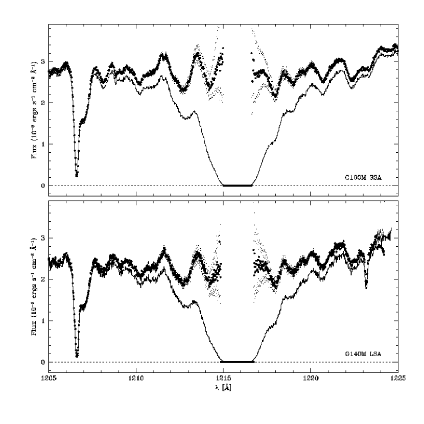
Figure 17: The best fit (filled circles) and $\pm 2\sigma$ (points) values for the reconstructed continuum in the G160M and G140M observations (top and bottom, respectively). The best-fit column density of H I along this sightline is $\log N({\rm H\;\mbox{\small I}})=19.87\pm 0.015$. The thick line at the center of the line profile shows the range over which we have not reconstructed the profile, i.e., the range over which the signal to noise is less than 10.

From our analysis of the GHRS observations of Ly$\alpha$ towards $\mu$ Col, we derive a column density of neutral hydrogen $\log N(\mbox{{H~{}I}})=19.87\pm 0.015$ ($\pm 1\sigma$ systematic). Figure 17 shows the observed and reconstructed intensities for the G160M observations. We also show the $\pm 2\sigma$ (systematic) reconstructed continua. The derivation of $N({\rm H\;\mbox{\small\rm I}})$ is relatively subjective. Given the complex undulating stellar continuum against which we are viewing the Ly$\alpha$ absorption, we feel a formal fitting procedure is unwarranted.

Estimating the errors in our column density determination is not a straightforward or easily quantifiable task. The undulations in the reconstructed continuum are primarily due to stellar absorption lines. The signal to noise ratios of our Ly$\alpha$ spectra are high enough that the systematic errors of the continuum reconstruction method (i.e., continuum placement, central velocity, etc.) almost certainly dominate the statistical errors (e.g., photon statistics, background subtraction, etc.) in our derivation. We have estimated $\pm 2\sigma$ systematic errors for the values of $N({\rm H\;\mbox{\small\rm I}})$ we judged to give the best continuum reconstruction by increasing and decreasing $N({\rm H\;\mbox{\small\rm I}})$ until we judge the resulting continuum reconstructions as highly implausable. In Figure 17 we display the best fit continuum reconstruction along with the $\pm 2\sigma$ reconstructions. One can see that these $\pm 2\sigma$ results are truly unacceptable. That the range of appropriate values is so small is a result of the high signal to noise and exceptional scattered light properties of the observations.

One problem in deriving the H I column density is determining the velocity alignment of the spectrum. We have used the lines of the N I triplet near $\lambda$1200 (e.g., see Figure 2) to give us a range of acceptable values for the velocity zero-point of our spectrum, but we have used the reconstructed wings of the H I Ly$\alpha$ profile themselves to fine-tune this determination. The assumption in this approach is that the absorption is symmetric. This may not be the case given complex component structure along the line of sight. Though the S II profile is reasonably approximated by a Gaussian fit (i.e., our turbulent broadening discussed above), we have in deriving our final number derived the thermal Gaussian profile with a detailed model of the component structure along the sightline. We use the results of our component fitting to the S II profile, with additional approximations for components 3, 4, and 5, as the kernel for the non-thermal structure along the sightline. The results of using this detailed model are almost indistinguishable from the simple Gaussian turbulent broadening model described above.

Because the derivation of $N({\rm H\;\mbox{\small\rm I}})$ relies heavily upon the very broad wings of the absorption profile, the precise details of the convolutions described here make little difference to the final result. As mentioned above, using a detailed component model as opposed to a simple Gaussian model for the non-thermal broadening gives indistinguishable results. Adopting temperatures in the range $100<T<10000$ K makes virtually no difference to the final continuum reconstruction. Even neglecting the smearing by the instrumental spread function makes only very negligible changes to the reconstructed continuum. Not only are the results we present quite robust to errors in these facets of our approach, but future works at comparable resolutions need not worry so much about the details of such complications when attempting to derive the H I column density along a given line of sight. Again, the keys to our ability to precisely derive the H I column density are the high signal-to-noise ratios of our data, the exceptional scattered light properties of the GHRS first-order gratings, and an appropriate (though not overly high) resolution.

Our derived value of $N({\rm H\;\mbox{\small\rm I}})$ is quite similar to past determinations. From IUE measurements of Ly$\alpha$, Diplas & Savage (1994) derive $\log N(\mbox{{H~{}I}})=19.88\pm 0.08$. Bohlin et al. (1978) derive $\log N(\mbox{{H~{}I}})=19.85\pm 0.08$ from Copernicus observations of Ly$\alpha$, and from Copernicus measurements of Lyman-$\beta$ and higher Lyman series absorption, York & Rogerson (1976) have estimated $\log N(\mbox{{H~{}I}})=19.9\pm 0.1$. The primary advantage of our derivation is that the errors are almost completely due to the systematics of the continuum reconstruction method applied to a star with undulating stellar absorption features $\sim 5-30\%$ deep.

The derived column density $\log N(\mbox{{H~{}I}})=19.87\pm 0.015$ contains contributions from the stellar photosphere as well as the interstellar medium. We must account for the stellar component if we are to very accurately derive the interstellar H I column density. Savage & Panek (1974) have shown that the observed equivalent widths of stellar Ly$\alpha$ absorption for nearby early-type stars are in agreement with the non-LTE predictions of Mihalas (1972a,b). Their work was used by Diplas & Savage (1994) to derive stellar contributions to the Ly$\alpha$ equivalent width based upon an empirical calibration using the Strömgren $[c_{1}]$ index. They suggest a contribution from the photosphere of $\mu$ Col of order $W_{\lambda}(\mbox{Ly$\alpha$})=2.95$ Å, equivalent to $\log N_{\rm HI}\equiv 18.27+\log W_{\lambda}(\mbox{Ly$\alpha$})=18.74$.

In this work we will estimate the contribution of stellar Ly$\alpha$ absorption by using the Mihalas (1972a,b) models presented in Savage & Panek (1974) to constrain the expected ratio of $W_{\lambda}(\mbox{Ly$\alpha$})/W_{\lambda}({\rm H}\beta)$. Using measurements of the H$\beta$ equivalent width by Buscombe (1969) we will then estimate the stellar contribution to $W_{\lambda}(\mbox{Ly$\alpha$})$. Using the data in Table 3 of Savage & Panek (1974) we find the ratio of these two hydrogen lines is well fit by a third order polynomial such that:

$$W_{\lambda}(\mbox{Ly$\alpha$})/W_{\lambda}({\rm H}\beta)=14.89-38.33\left(\frac{T_{eff}}{30,000\ {\rm K}}\right)+39.53\left(\frac{T_{eff}}{30,000\ {\rm K}}\right)^{2}-15.12\left(\frac{T_{eff}}{30,000\ {\rm K}}\right)^{3}.$$ (A7)

For $\mu$ Col we predict $W_{\lambda}(\mbox{Ly$\alpha$})/W_{\lambda}({\rm H}\beta)\approx 0.418$. The measured H$\beta$ equivalent width from the photosphere of $\mu$ Col is $W_{\lambda}({\rm H}\beta)=1.77$ Å (Buscombe 1969), suggesting a stellar contribution to the Ly$\alpha$ equivalent width of $W_{\lambda}(\mbox{Ly$\alpha$})\approx 0.74$ Å. This is equivalent to $\log N_{\rm HI}\approx 18.14$. Thus the stellar contribution should represent $\approx 0.01$ dex of the total. We adopt a final interstellar column density to the star $\mu$ Col of $\log N_{\rm HI}=19.86\pm 0.015$ ($1\sigma$ systematic).

Appendix B DERIVATION OF THE LARGE SCIENCE APERTURE LINE SPREAD FUNCTION

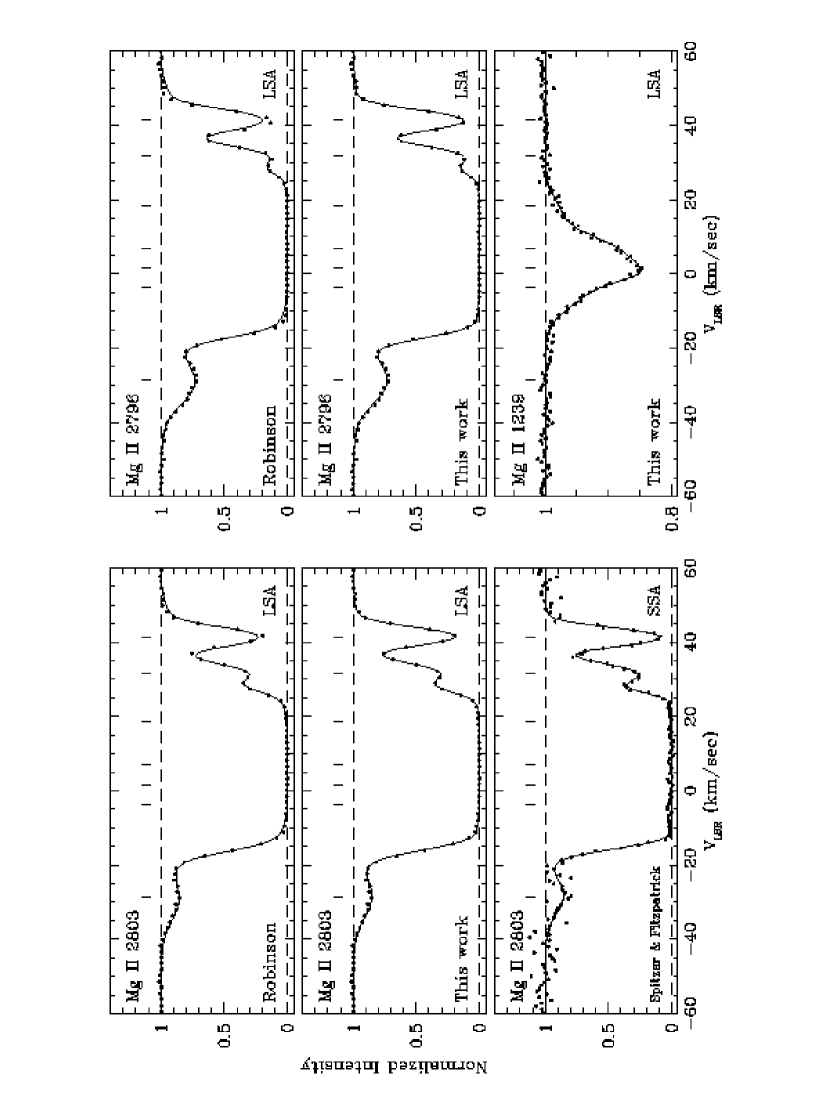
Figure 18: A comparison of the best-fit component models for the Mg II $\lambda\lambda 2796$ and 2803 Å transitions using the Robinson et al. LSF (1998; top row), that derived in this work (middle row), and the SSA data plus Spitzer & Fitzpatrick (1993) LSF. Also shown in the bottom row is the best fit model for Mg II $\lambda 1239$ Å transition derived simultaneously with the stronger transitions using our derived LSF. The central velocities of the individual components are marked as ticks above the profiles.

In the process of attempting to fit component models to our interstellar line profiles, we have come to the conclusion that the LSF presented by Robinson et al. (1998) for the LSA is not appropriate at most wavelengths covered by the GHRS, evidenced by our inability to adequately fit model profiles to the narrow, often deep, component 4. Figure 18 shows the best fit model for Mg II $\lambda\lambda$2796 and 2803 in the top row when using the LSF suggested by Robinson et al. (1998). Our best fit component models for Mg II at $\lambda\lambda$2796 and 2803 using the Robinson et al. LSF were unable to match the depth of the core of component 4, while at the same time they provided too much absorption in the wings of the profile. Furthermore, when we fit the pre-COSTAR observations of Mg II $\lambda$2803 taken through the SSA using the spread function derived by Spitzer & Fitzpatrick (1993) and Fitzpatrick (priv. comm.), we found significant discrepancies in the derived column densities for components 3 and 4, which are both very narrow and deep. Using the Robinson et al. LSF we derived a column density $\log N_{4}(\mbox{{Mg~{}II}})=13.22\pm 0.09$; using the SSA observations and the LSF of Fitzpatrick & Spitzer we derived $\log N_{4}(\mbox{{Mg~{}II}})=12.86\pm 0.05$, more than a factor of two different. Also, the derived $b$-values were slightly different: $b_{4}=2.0\pm 0.3$ km s^-1 using the SSA observations and $b_{4}=1.54\pm 0.15$ km s^-1 using the LSA observations. We found similar discrepancies comparing the SSA and LSA observations of O I. However, the SSA and LSA results agreed relatively well when comparing fits of the Si II $\lambda$1304 transition. We believe this is because component 4 is not as deep in this line as the others. Thus the differences in the LSF seem to give significantly different results only for strong, very narrow absorption features.

We have attempted to rederive the line spread function for the LSA. Though the problem is poorly constrained by the current dataset, we have pieced together a spread function that is able to match the SSA results and provide good fits to the data. To begin we have fit the Robinson et al. (1998) spread function with two Gaussians: a narrow “core” and a broad “halo” component. Table 12 gives the FWHMs (in diodes) and relative areas of these Gaussians. Our approach has been to assume a two-component Gaussian model is a valid approximation to the LSA spread function, and that the values of the FWHM from the Robinson et al. LSF are reasonable. We assume the widths of the core and halo Gaussians in diode-space are constant. The effective resolution changes with placement of the diode array in the echelle due to differences in the mapping of wavelengths to diode space. Our free parameter in the fit is the relative area of the core and halo components. We have proceeded by fitting the SSA data for O I, Si II, Mg II, and Fe II using the Fitzpatrick & Spitzer LSF. Then we have held the results of these fits constant and applied them to our LSA observations using varying values of the relative power of the core and halo components of our LSF. For each transition of these species that showed component 4 strongly, we have derived a best fit value for the relative power of the halo to the LSF. Figure 19 shows our derived spread function with the Robinson et al. (1998) and Spitzer & Fitzpatrick (1993) LSFs at $\lambda 1900$ Å.

The extended wings of the LSF in the LSA are a result of the broad wings of the point spread function from the aberrated primary (plus COSTAR) being allowed to enter the spectrograph through the $1\farcs 74\times 1\farcs 74$ LSA. For the SSA, which effectively blocks the far wings of the telescope point spread function, the broad component adopted by Fitzpatrick & Spitzer is a result of aberrations in the internal optics of the spectrograph and effects in the detector. The relative power of the broad component is much greater in the spread function for the LSA than for the SSA. We have fit the fractional contribution of the halo component, $f_{halo}$, to the total as a function of wavelength with the following function:

$$f_{halo}=0.486-(2.89\times 10^{-4})\lambda+(5.52\times 10^{-8})\lambda^{2}.$$ (B1)

We find that this prescription gives results that agree in column density and $b$-value with fits to the SSA data using the Fitzpatrick & Spitzer SSA spread function. The best fit profile using this profile is also better able to reproduce the data than the Robinson et al. LSF. Figure 18 shows the results of the component fits for the Mg II lines. The top row shows the best fit component model using the Robinson spread function for the Mg II lines near $\lambda$2800, the middle row shows the best fit using our derived spread function, and the bottom row shows the fit to the SSA data using the Spitzer & Fitzpatrick (1993) spread function. Also shown in the bottom row is the fit obtained simultaneously for the Mg II $\lambda$1239 transition using our derived LSF. The tick marks show the locations of our model interstellar components. When examining the fit to component 4 near $v_{\rm LSR}=+41$ km s^-1, it is clear that our LSF provides a better fit to this strong, narrow component. Furthermore, it provides results consistent with those derived using the SSA data.

While our empirically-derived LSF is able to match the SSA data, we do not wish to suggest the LSA spread function is well understood. Our fit is consistent with the available data, though the problem is ill-constrained, particularly in the wavelength range $1600<\lambda<2300$ Å, where we have no data. The true LSF of the LSA is likely more complex than the two Gaussian model we have adopted. Further, the true spread function may be a function of the positioning of the star within the LSA. It is important to realize that the adoption of a specific shape for the instrumental profile can have important consequences when trying to derive accurate column densities for narrow, deep lines. When possible, investigators interested in deriving the column densities of such components should use the SSA, for which the spread function has been better characterized (e.g., Spitzer & Fitzpatrick 1993) and is better behaved. When using data taken through the LSA for such work, one should investigate the consequences of adopting slightly different spread functions. In our case the values derived for the column densities of O I and Mg II were different by factors of 1.5 to 2.5 between the different spread functions.

Table 1: Velocities and Conditions in the Absorbing Regions Towards $\mu$ Columbae

Region	$v_{\rm LSR}$	$\Delta v$	$T_{e}$	$n_{e}$	Previous
Number	[km s-1]	[km s-1]	[K]	[cm-3]	ID
1	+3	$-$17.0 to 15.5	$6,200\pm 300$	$0.27\pm 0.05$	A
2	+20.1	15.5 to 29.0	$6,900\pm 600$	$0.31\pm 0.13$	B
3	+31.0	29.0 to 37.5	$\lesssim 10,000$	$\cdots$	D
4	+41.2	37.5 to 47.0	$4,000\pm 700$	$0.64\pm 0.12$	C
5	$-28.8$	$-45.0$ to $-17.0$	$\lesssim 36,000$	$\cdots$	$\cdots$

Table 2: Log of GHRS Observations

Spectral Range	Rootname	Exp.	Mode	Aper.	dc	Species
[Å]		[sec]	& Order			Detected
1116-1124	Z2X30108T	81.6	G140M/1	LSA	0.0	Fe II, Fe III
	Z2X30109T	81.6	G140M/1	LSA
1131-1137	Z2C0011AP	108.8	A/49	LSA	0.011	N I, Fe II
1142-1148	Z2AF011AT	108.8	A/49	LSA	0.061:	Fe II
	Z2C0030RT	108.8	A/49	LSA
	Z308010OT	108.8	A/49	LSA
	Z3JN010OT	108.8	A/49	LSA
1149-1153	Z2AF020RT	108.8	A/49	LSA	0.061:	P II
	Z2C0010QP	108.8	A/49	LSA
	Z2C0021AP	108.8	A/49	LSA
1154-1161	Z2C00119P	108.8	A/48	LSA	0.058:	C I
1157-1163	Z2C0041AT	108.8	A/49	LSA	0.011:	C I
1184-1191	Z2AF010PT	108.8	A/47	LSA	0.000	C I, Si II, S III
	Z2C0020PP	108.8	A/47	LSA
1191-1197	Z2AF0118T	108.8	A/47	LSA	0.038	Si II
	Z2AF021CT	108.8	A/47	SSA
	Z2C0030PT	108.8	A/47	LSA
1195-1230	Z2AN020AT	54.4	G160M/1	SSA	0.0	H I
1197-1225	Z2XE010DT	27.2	G140M/1	LSA	0.0	H I
1197-1225	Z2XE0117T	27.2	G140M/1	SSA	0.0	H I
1197-1200	Z2AF020PT	108.8	A/47	LSA	0.038:	N I, Mn II
1200-1203	Z2C00218P	108.8	A/47	LSA	0.035	N I
1206-1212	Z2AZ010MT	1740.8	A/46	SSA	0.027	Si III
1237-1244	Z2AZ010CT	1088.0	A/45	LSA	0.049:	N V, Mg II
	Z2AZ010OT	1088.0	A/45	SSA
1249-1256	Z2AF020MT	27.2	A/45	LSA	0.049:	S II
	Z2C00215P	27.2	A/45	LSA
1259-1262	Z2C0040MT	27.2	A/45	LSA	0.033	S II
1259-1267	Z2C00114P	27.2	A/44	LSA	0.026	Si II∗
1271-1278	Z2AF0114T	27.2	A/44	LSA	0.046:	C I
1301-1308	Z2AF0113T	27.2	A/44	LSA	0.050	O I, Si II, P II
	Z2AF0217T	27.2	A/44	LSA
	Z2C0030KT	27.2	A/44	LSA
	Z308010HT	27.2	A/44	LSA
1313-1320	Z2C0010JP	27.2	A/43	LSA	0.050:	Ni II
	Z2C0040KT	27.2	A/43	LSA
1326-1333	Z2AF010JT	27.2	A/42	LSA	0.041:	C I
	Z2C0020JP	27.2	A/42	LSA
1332-1339	Z2AF0112T	27.2	A/42	LSA	0.041	C II, C II∗
	Z2AF0216T	27.2	A/42	SSA
	Z2C0030JT	27.2	A/42	LSA
	Z308010GT	27.2	A/42	LSA
1364-1372	Z2AF0111T	27.2	A/41	LSA	0.039:	Ni II
	Z2AF0215T	27.2	A/41	SSA
	Z2C0030IT	27.2	A/41	LSA
	Z308010FT	27.2	A/41	LSA
1526-1534	Z2C0040DT	54.4	A/37	LSA	0.055	Si II
	Z2C0040ET	27.2	A/37	LSA
1554-1562	Z2AF010VT	108.8	A/36	LSA	0.031:	C I
	Z2AF020ZT	108.8	A/36	SSA
	Z2C0030CT	54.4	A/36	LSA
1606-1614	Z2AF020BT	108.8	A/35	LSA	0.030:	Fe II
	Z2C0020UP	54.4	A/35	LSA
1653-1662	Z2AF020AT	108.8	A/34	LSA	0.030:	C I
	Z2C0020TP	54.4	A/34	LSA
1668-1676	Z2C0040TT	54.4	A/34	LSA	0.030	Al II
1706-1712	Z2AF0209T	108.8	A/33	LSA	0.029:	Ni II
	Z2CX011KT	27.2	B/33	LSA	0.045:
	Z2C0020SP	54.4	A/33	LSA	0.029:
	Z2D4021JT	54.4	B/33	LSA	0.045:
1740-1749	Z2D4020MT	54.4	B/32	LSA	0.043:	Ni II
1805-1809	Z2CX010MT	27.2	B/31	LSA	0.041:	Si II
	Z2D40211T	54.4	B/31	LSA
1846-1857	Z2D40118T	54.4	B/30	LSA	0.039:	Al III
1860-1866	Z2CX010LT	27.2	B/30	LSA	0.039:	Al III
	Z2D4020KT	54.4	B/30	LSA
2017-2027	Z2D4030IT	54.4	B/28	LSA	0.035:	Mg I, Zn II
2052-2061	Z2D40115T	54.4	B/27	LSA	0.033:	Cr II
2062-2063	Z2D40115T	54.4	B/27	LSA	0.033:	Cr II
	Z2D4020HT	54.4	B/27	LSA
2063-2074	Z2D4020HT	54.4	B/27	LSA	0.033:	Cr II
2242-2254	Z23L040FT	57.6	B/25	LSA	0.030:	Fe II
	Z29I060FT	57.6	B/25	LSA
	Z2D4021BT	54.4	B/25	LSA
	Z308020DT	115.2	B/25	LSA
	Z3JN020DT	115.2	B/25	LSA
2259-2264	Z2CX011CT	27.2	B/25	LSA	0.030:	Fe II
	Z2D4030FT	54.4	B/25	LSA
2335-2348	Z23L040ET	57.6	B/24	LSA	0.031	Fe II
	Z308020CT	115.2	B/24	LSA
	Z3JN020CT	115.2	B/24	LSA
2364-2376	Z2D4030UT	54.4	B/24	LSA	0.028:	Fe II
2567-2581	Z2D4030CT	54.4	B/22	LSA	0.017:	Mn II
2575-2590	Z2D4030ST	54.4	B/22	LSA	0.017:	Fe II
2590-2603	Z2D40318T	54.4	B/22	LSA	0.017	Mn II, Fe II
2792-2802	Z23L0413T	28.8	B/20	LSA	0.015	Mg II
	Z29I0613T	28.8	B/20	LSA
2802-2807	Z23L0413T	28.8	B/20	LSA	0.015	Mg II
	Z23L0414T	28.8	B/20	LSA
	Z23L040AT	57.6	B/20	LSA
	Z29I060AT	57.6	B/20	LSA
	Z29I0613T	28.8	B/20	LSA
	Z29I0614T	28.8	B/20	LSA
2852-2857	Z23L0418T	28.8	B/20	LSA	0.015:	Mg I
	Z23L0419T	28.8	B/20	LSA
	Z29I0618T	28.8	B/20	LSA

Table 3: Integrated Equivalent Widths

	IP	IP				Wλ [mÅ]
Species	$\chi^{i-1}$	$\chi^{i}$	$\lambda_{vac}$	log $\lambda f$	Ref.	Comp 1	Comp 2	Comp 3	Comp 4	S/N
	[eV]	[eV]	[Å]			(3 km s-1)	(20 km s-1)	(31 km s-1)	(41 km s-1)
C I	$\cdots$	11.26	1328.833	1.887	1	$7.2\pm 0.5$	$<2.2$	$<1.9$	$<1.9$	48
			1560.309	2.099	1	$12.0\pm 0.7$	$2.7\pm 0.5$	$<1.7$	$<1.7$	64
			1656.928	2.367	1	$18.8\pm 2.4$	$3.6\pm 1.5$	$<3$	$<3$	26
C I∗	$\cdots$	11.26	1656.267	1.987	1	$2.4\pm 0.9$	$<3$	$<3$	$<3$	42
			1657.907	1.890	1	$4.8\pm 2.0$	$<4$	$<4$	$<4$	32
C I∗∗	$\cdots$	11.26	1277.550	2.016	1	$<3$	$<2.0$	$<1.7$	$<1.7$	51
			1561.438	2.023	1	$<4$	$<3$	$<3$	$<3$	42
			1658.121	1.765	1	$<5$	$<4$	$<4$	$<4$	31
C II	11.26	24.38	1334.532	2.232	1	$155\pm 9$	$56.0\pm 1.1$	$65.0\pm 1.3$	$28.3\pm 0.6$	56
C II∗	11.26	24.38	1335.708	2.186	1	$132\pm 3$	$23.6\pm 0.6$	$2.3\pm 0.6$	$3.5\pm 0.5$	31
N I	$\cdots$	14.53	1134.165	1.182	1	$79.2\pm 2.0$	$28.0\pm 1.0$	0.$<3$	0.$<3$	12
			1134.415	1.483	1	$96.2\pm 2.1$	$24.9\pm 1.0$	$<3.3$	$2.9\pm 1.0$	12
			1134.980	1.660	1	$106.0\pm 2.2$	$23.8\pm 0.9$	$<2.4$	$5.0\pm 0.8$	14
			1199.550	2.202	1	$118\pm 3$	$34.9\pm 0.8$	$\cdots$	$14.8\pm 0.8$	27
			1200.223	2.026	1	$116.0\pm 2.3$	$34.3\pm 0.7$	$\cdots$	$11.3\pm 0.4$	46
			1200.710	1.725	1	$109.2\pm 2.2$	$32.2\pm 0.7$	$\cdots$	$7.7\pm 0.4$	49
O I	$\cdots$	13.62	1302.169	1.804	1	$137\pm 3$	$52.6\pm 1.1$	$16.4\pm 0.4$	$22.8\pm 0.5$	54
			1355.598	-2.772	1	$<3$	$<2.3$	$<2.0$	$<2.0$	46
Mg I	$\cdots$	7.65	2026.477	2.369	1	$16.5\pm 1.7$	$2.0\pm 0.5$	$<1.5$	$<1.5$	44
			2852.964	3.718	1	$207\pm 4$	$44.8\pm 1.0$	$2.2\pm 0.4$	$3.9\pm 0.5$	80
Mg II	7.65	15.04	1239.925	-0.100	2	$9.82\pm 0.24$	$0.79\pm 0.09$	0$<0.3$	0$<0.3$	195
			1240.395	-0.401	2	$5.47\pm 0.18$	$0.36\pm 0.09$	$<0.18$	$<0.18$	217
			2796.352	3.234	1	$307\pm 6$	$117\pm 3$	$59.4\pm 1.2$	$49.9\pm 1.1$	111
			2803.531	2.933	1	$297\pm 6$	$112.1\pm 2.3$	$46.3\pm 1.0$	$44.2\pm 0.9$	136
Al II	5.99	18.83	1670.787	3.486	1	$148\pm 3$	$55.7\pm 1.3$	$9.3\pm 1.0$	$6.5\pm 1.0$	16
Al III	18.83	28.45	1854.716	3.017	1	$15.0\pm 2.0$	$<3.0$	$<3.0$	$<3.0$	30
			1862.790	2.716	1	$9.9\pm 1.5$	$<2.4$	$<2.4$	$<2.4$	35
Si II	8.15	16.35	1190.416	2.474	1	$116.0\pm 2.3$	$48.3\pm 1.0$	$12.1\pm 0.3$	$12.3\pm 0.3$	54
			1193.290	2.775	1	$124\pm 3$	$50.0\pm 1.0$	$19.0\pm 0.5$	$17.0\pm 0.4$	48
			1304.370	2.050	3,4	$121\pm 3$	$42.5\pm 0.9$	$6.91\pm 0.24$	$8.5\pm 0.3$	57
			1526.707	2.225	3,4	$148\pm 3$	$56.3\pm 1.2$	$11.9\pm 0.5$	$12.4\pm 0.6$	27
			1808.013	0.596	5,4	$61.2\pm 1.6$	$6.5\pm 0.2$	$<1.5$	$<1.5$	36
Si II∗	8.15	16.35	1264.738	3.058	1	$3.60\pm 1.16$	$<1.8$	$<1.8$	$<1.8$	33
Si III	16.35	33.49	1206.500	3.304	1	$126\pm 3$	$40.9\pm 0.9$	$10.7\pm 0.5$	$1.4\pm 0.5$	76
P II	10.49	19.72	1152.818	2.435	1	$53.2\pm 1.4$	$4.9\pm 0.5$	$<1.5$	$<1.5$	32
			1301.874	1.351	1	$6.6\pm 0.6$	$\cdots$	$\cdots$	$\cdots$	55
S II	10.36	23.33	1250.534	0.834	1	$68.6\pm 1.4$	$7.4\pm 0.4$	$<0.9$	$<0.9$	40
			1253.811	1.135	1	$90.9\pm 1.8$	$11.3\pm 0.4$	$<0.9$	$<0.9$	43
			1259.519	1.311	1	$104.6\pm 2.1$	$20.0\pm 0.6$	$<1.3$	$<1.2$	36
S III	23.33	34.83	1190.208	1.421	1	$16.3\pm 0.6$	$<0.9$	$<0.9$	$\cdots$	58
Cr II	6.77	16.50	2056.254	2.334	6	$12.2\pm 1.3$	$4.2\pm 0.7$	$<1.5$	$<1.5$	43
			2062.234	2.206	6	$6.7\pm 1.3$	$3.5\pm 0.6$	$<1.2$	$<1.2$	73
			2066.161	2.027	6	$6.0\pm 0.9$	$2.6\pm 0.5$	$<1.2$	$<1.2$	48
Mn II	7.44	15.64	1197.184	2.273	1	$5.6\pm 0.4$	$1.0\pm 0.3$	$<0.6$	$<0.6$	42
			2576.877	2.956	1	$55.8\pm 1.3$	$10.9\pm 0.4$	$1.6\pm 0.4$	$1.1\pm 0.4$	68
			2594.499	2.847	1	$43.6\pm 1.1$	$8.7\pm 0.5$	$<1.2$	$<1.2$	60
Fe II	7.87	16.16	1133.665	-1.222	1	$9.5\pm 2.2$	$4.5\pm 1.1$	$<3$	$<3$	13
			1143.226	1.182	1	$24.7\pm 1.0$	$10.1\pm 0.4$	$<2.2$	$<2.2$	35
			1144.938	2.080	1	$75.1\pm 1.7$	$32.1\pm 0.8$	$3.6\pm 0.6$	$2.1\pm 0.6$	31
			1608.451	1.998	7,8	$100.3\pm 2.1$	$36.6\pm 0.8$	$3.6\pm 0.5$	$3.9\pm 0.5$	35
			2249.877	0.612	9,10	$10.2\pm 0.3$	$3.96\pm 0.20$	$<0.6$	$<0.6$	218
			2260.780	0.742	9,10	$15.0\pm 0.5$	$6.9\pm 0.3$	$<0.9$	$<0.9$	97
			2344.214	2.410	1	$204\pm 4$	$70.0\pm 1.4$	$16.0\pm 0.3$	$11.7\pm 0.3$	236
			2374.461	1.889	7,10	$125\pm 3$	$47.7\pm 1.0$	$5.3\pm 0.3$	$4.1\pm 0.3$	65
			2586.650	2.248	7,10	$196\pm 4$	$74.0\pm 1.5$	$11.4\pm 0.4$	$9.8\pm 0.4$	60
			2600.173	2.765	1	$238\pm 5$	$98.9\pm 2.0$	$28.7\pm 0.7$	$22.1\pm 0.6$	51
Fe III	16.16	30.65	1122.526	1.947	1	$19\pm 4$	$\cdots$	$\cdots$	$\cdots$	24
Ni II	7.64	18.17	1317.217	2.012	1,11	$6.8\pm 0.7$	$3.6\pm 0.4$	$<1.2$	$<1.2$	44
			1370.132	2.023	11,12	$8.1\pm 0.5$	$3.4\pm 0.3$	$<0.6$	$<0.6$	68
			1709.600	1.784	12	$4.9\pm 1.0$	$3.4\pm 0.5$	$<1.2$	$<1.2$	44
			1741.569	1.858	12	$14.5\pm 1.6$	$5.5\pm 0.9$	$<2.4$	$<2.4$	21
Cu II	7.73	20.29	1358.773	2.713	1	$<3$	$<2.2$	$<1.9$	$<1.9$	50
Zn II	9.39	17.96	2026.136	2.996	6	$52.5\pm 1.6$	$4.5\pm 0.8$	$\cdots$	$\cdots$	46
			2062.664	2.723	6	$26.5\pm 1.1$	$2.2\pm 0.5$	$<1.2$	$<1.2$	65

References. — (1) Morton (1991); (2) Fitzpatrick (1997); (3) Spitzer & Fitzpatrick (1993); (4) Dufton, et al. (1983, 1992); (5) Bergeson & Lawler (1993a); (6) Bergeson & Lawler (1993b); (7) Cardelli & Savage (1995); (8) Bergeson, et al. (1996a); (9) Bergeson, et al. (1994); (10) Bergeson, et al. (1996b); (11) Fedchak & Lawler (1999); (12) Zsargó & Federman (1997)

Table 4: Integrated Apparent Column Densities

		Log(Na) [cm -2]
Species	$\lambda_{vac}$	Comp 1	Comp 2	Comp 3	Comp 4
	[Å]	(3 km s-1)	(20 km s-1)	(31 km s-1)	(41 km s-1)
C I	1328.833	$12.92\pm 0.04$	$\cdots$	$\cdots$	$\cdots$
C I	1560.309	$12.87\pm 0.03$	$12.21\pm 0.09$	$\cdots$	$\cdots$
C I	1656.928	$12.79\pm 0.07$	$\cdots$	$\cdots$	$\cdots$
C I∗	1656.267	$12.46^{+0.11}_{-0.15}$	$\cdots$	$\cdots$	$\cdots$
C I∗	1657.907	$12.65^{+0.15}_{-0.24}$	$\cdots$	$\cdots$	$\cdots$
C II	1334.532	$\times\times\times$	$\times\times\times$	$\times\times\times$	$>13.5$
C II∗	1335.708	$\times\times\times$	$>13.3$	$12.13\pm 0.10$	$12.32\pm 0.14$
N I	1134.165	$\times\times\times$	$\times\times\times$	$\cdots$	$\cdots$
N I	1134.415	$\times\times\times$	$\times\times\times$	$\cdots$	$13.02^{+0.13}_{-0.18}$0.
N I	1134.980	$\times\times\times$	$\times\times\times$	$\cdots$	$13.08\pm 0.08$
N I	1199.550	$\times\times\times$	$\times\times\times$	$\cdots$	$12.95\pm 0.10$
N I	1200.223	$\times\times\times$	$\times\times\times$	$\cdots$	$13.09\pm 0.02$
N I	1200.710	$\times\times\times$	$\times\times\times$	$\cdots$	$13.19\pm 0.10$
O I	1302.169	$\times\times\times$	$\times\times\times$	$13.49\pm 0.02$	$13.72\pm 0.02$
Mg I	2026.477	$12.63\pm 0.05$	$11.72\pm 0.11$ 0.	$\cdots$	$\cdots$
Mg I	2852.964	$12.54\pm 0.02$	$11.68\pm 0.02$	$10.23\pm 0.09$	$10.48\pm 0.06$
Mg II	1239.925	$15.08\pm 0.02$	$13.96\pm 0.05$	$\cdots$	$\cdots$
Mg II	1240.395	$15.11\pm 0.03$	$13.92^{+0.10}_{-0.12}$0.	$\cdots$	$\cdots$
Mg II	2796.352	$\times\times\times$	$\times\times\times$	$12.44\pm 0.02$	$12.35\pm 0.02$
Mg II	2803.531	$\times\times\times$	$\times\times\times$	$12.52\pm 0.02$	$12.53\pm 0.02$
Al II	1670.787	$\times\times\times$	$\times\times\times$	$11.30\pm 0.05$	$11.21\pm 0.06$
Al III	1854.716	$11.97\pm 0.07$	$\cdots$	$\cdots$	$\cdots$
Al III	1862.790	$12.08\pm 0.07$	$\cdots$	$\cdots$	$\cdots$
Si II	1190.416	$\times\times\times$	$\times\times\times$	$12.70\pm 0.02$	$12.70\pm 0.03$
Si II	1193.290	$\times\times\times$	$\times\times\times$	$12.70\pm 0.02$	$12.60\pm 0.02$
Si II	1304.370	$\times\times\times$	$\times\times\times$	$12.79\pm 0.03$	$12.87\pm 0.03$
Si II	1526.707	$\times\times\times$	$\times\times\times$	$12.80\pm 0.03$	$12.82\pm 0.03$
Si II	1808.013	$15.10\pm 0.02$	$14.05\pm 0.06$	$\cdots$	$\cdots$
Si II∗	1264.738	$11.47^{+0.12}_{-0.17}$0.	$\cdots$	$\cdots$	$\cdots$
Si III	1206.500	$\times\times\times$	$>12.67$	$11.81\pm 0.03$	$10.84^{+0.16}_{-0.21}$0.
P II	1152.818	$13.46\pm 0.02$	$12.29\pm 0.05$	$\cdots$	$\cdots$
P II	1301.874	$13.42\pm 0.04$	$\cdots$	$\cdots$	$\cdots$
S II	1250.534	$15.19\pm 0.02$	$14.04\pm 0.03$	$\cdots$	$\cdots$
S II	1253.811	$15.17\pm 0.02$	$13.97\pm 0.03$	$\cdots$	$\cdots$
S II	1259.519	$15.13\pm 0.02$	$14.08\pm 0.03$	$\cdots$	$\cdots$
S III	1190.208	$13.82\pm 0.02$	$\cdots$	$\cdots$	$\cdots$
Cr II	2056.254	$12.51\pm 0.05$	$12.05\pm 0.07$	$\cdots$	$\cdots$
Cr II	2062.234	$12.37\pm 0.09$0.	$\cdots$	$\cdots$	$\cdots$
Cr II	2066.161	$12.50\pm 0.07$	$12.14^{+0.07}_{-0.09}$0.	$\cdots$	$\cdots$
Mn II	1197.184	$12.44\pm 0.04$	$\cdots$	$\cdots$	$\cdots$
Mn II	2576.877	$12.50\pm 0.02$	$11.75\pm 0.03$	$10.89^{+0.09}_{-0.12}$ 0.	$10.67^{+0.13}_{-0.20}$ 0.
Mn II	2594.499	$12.48\pm 0.02$	$11.75\pm 0.03$	$\cdots$	$\cdots$
Fe II	1133.665	$14.18\pm 0.09$	$13.85^{+0.10}_{-0.12}$	$\cdots$	$\cdots$
Fe II	1143.226	$14.27\pm 0.07$	$13.87\pm 0.05$	$\cdots$	$\cdots$
Fe II	1144.938	$14.15\pm 0.03$	$13.70\pm 0.02$	$\cdots$	$\cdots$
Fe II	1608.451	$14.10\pm 0.02$	$13.63\pm 0.02$	$12.43\pm 0.06$	$12.46\pm 0.07$
Fe II	2249.877	$14.11\pm 0.02$	$13.70\pm 0.02$	$\cdots$	$\cdots$
Fe II	2260.780	$14.15\pm 0.02$	$13.81\pm 0.02$	$\cdots$	$\cdots$
Fe II	2344.214	$\times\times\times$	$13.52\pm 0.02$	$12.55\pm 0.02$	$12.41\pm 0.02$
Fe II	2374.461	$14.09\pm 0.03$	$13.67\pm 0.02$	$12.54\pm 0.04$	$12.43\pm 0.04$
Fe II	2586.650	$14.10\pm 0.02$	$13.61\pm 0.02$	$12.51\pm 0.03$	$12.43\pm 0.03$
Fe II	2600.173	$\times\times\times$	$\times\times\times$	$12.50\pm 0.02$	$12.35\pm 0.02$
Fe III	1122.526	13.37${}^{+0.09}_{-0.11}$0.	$\cdots$	$\cdots$	$\cdots$
Ni II	1317.217	$12.77\pm 0.05$	$12.50\pm 0.05$	$\cdots$	$\cdots$
Ni II	1370.132	$12.82\pm 0.03$	$12.46\pm 0.04$	$\cdots$	$\cdots$
Ni II	1709.600	$12.73\pm 0.09$0.	$12.58\pm 0.07$	$\cdots$	$\cdots$
Ni II	1741.569	$13.16\pm 0.06$	$12.71\pm 0.07$	$\cdots$	$\cdots$
Zn II	2026.136	$12.56\pm 0.03$	$11.35\pm 0.09$0.	$\cdots$	$\cdots$
Zn II	2062.664	$12.48\pm 0.03$	$11.38\pm 0.09$	$\cdots$	$\cdots$

Table 5: Component Fitting Column Densities and $b$-values

	Comp 1		Comp 2			Comp 3			Comp 4			Comp 5
Species	$\log N(X)$		$b$	$\log N(X)$		$b$	$\log N(X)$		$b$	$\log N(X)$		$b$	$\log N(X)$
$X$	[cm-2]		[km s-1]	[cm-2]		[km s-1]	[cm-2]		[km s-1]	[cm-2]		[km s-1]	[cm-2]
C II	$\times\times\times$		$\times\times\times$	$\times\times\times$		$\times\times\times$	$\times\times\times$		$3.0\pm 0.5$	$13.75\pm 0.05$		$7.0\pm 0.9$	$13.37\pm 0.10$
C II∗	$\times\times\times$		$3.5\pm 0.5$	$13.23\pm 0.03$		$\cdots$	$\cdots$		$2.4\pm 1.5$	$12.36\pm 0.05$		$\cdots$	$\cdots$
N I	$\times\times\times$		$4.1\pm 0.6$	$14.25\pm 0.08$		$\cdots$	$\cdots$		$2.17\pm 0.20$	$13.17\pm 0.02$		$\cdots$	$\cdots$
O I	$\times\times\times$		$3.9\pm 0.6$	$14.55\pm 0.05$		$4.2\pm 0.7$	$13.58\pm 0.03$		$2.58\pm 0.12$	$13.83\pm 0.02$		$\cdots$	$\cdots$
Mg I	$12.59\pm 0.05$		$2.60\pm 0.18$	$11.72\pm 0.02$		$\cdots$	$10.28\pm 0.11$		$\cdots$	$10.52\pm 0.04$		$\cdots$	$\cdots$
Mg II	$15.09\pm 0.20$		$4.9\pm 1.5$	$13.95\pm 0.12$		$2.6\pm 0.3$	$12.50\pm 0.02$		$1.82\pm 0.09$	$12.82\pm 0.02$		$7.5\pm 1.1$	$11.98\pm 0.02$
Al II	$\times\times\times$		$3.5\pm 0.8$	$12.64\pm 0.05$		2.65	$11.47\pm 0.05$		1.74	$11.27\pm 0.06$		$\cdots$	$\cdots$
Si II	$15.13\pm 0.11$		$3.6\pm 0.6$	$13.98\pm 0.05$		$2.7\pm 0.4$	$12.78\pm 0.02$		$1.67\pm 0.09$	$12.85\pm 0.02$		$4.4^{+4.9}_{-2.3}$	$11.64\pm 0.10$
Si III	$\times\times\times$		$4.6\pm 2.0$	$12.65\pm 0.08$		$3.34\pm 1.7$	$11.83\pm 0.10$		$\cdots$	$10.67\pm 0.22$		$7.5\pm 1.0$	$12.29\pm 0.03$
P II	$13.50\pm 0.15$		3.6	$11.98\pm 0.13$		$\cdots$	$\cdots$		$\cdots$	$\cdots$		$\cdots$	$\cdots$
S II	$15.24\pm 0.05$		$5.0\pm 0.7$	$13.82\pm 0.02$		$\cdots$	$\cdots$		$\cdots$	$\cdots$		$\cdots$	$\cdots$
Cr II	$12.48\pm 0.07$		3.0	$12.03\pm 0.05$		$\cdots$	$\cdots$		$\cdots$	$\cdots$		$\cdots$	$\cdots$
Mn II	$12.52\pm 0.10$		$3.0\pm 1.0$	$11.61\pm 0.05$		1.76	$10.82\pm 0.09$		1.18	$10.55\pm 0.14$		$\cdots$	$\cdots$
Fe II	$14.13\pm 0.02$		$2.75\pm 0.07$	$13.78\pm 0.02$		$1.76\pm 0.14$	$12.63\pm 0.02$		$1.18\pm 0.11$	$12.61\pm 0.02$		$3.9^{+5.0}_{-2.2}$	$11.34\pm 0.10$
Ni II	$12.86\pm 0.08$		2.79	$12.35\pm 0.04$		$\cdots$	$\cdots$		$\cdots$	$\cdots$		$\cdots$	$\cdots$
Zn II	$12.55\pm 0.08$		2.79	$11.16\pm 0.08$		$\cdots$	$\cdots$		$\cdots$	$\cdots$		$\cdots$	$\cdots$

Table 6: Component Fitting Velocities

	Comp 2		Comp 3		Comp 4		Comp 5
Species	$v_{\rm LSR}$		$v_{\rm LSR}$		$v_{\rm LSR}$		$v_{\rm LSR}$
$X$	[km s-1]		[km s-1]		[km s-1]		[km s-1]
C II	$\cdots$		$\cdots$		$41.25\pm 0.12$		$-28.0\pm 0.05$
C II∗	$20.18\pm 0.15$		$\cdots$		$41.7\pm 0.3$		$\cdots$
N I	$18.2\pm 0.5$		$\cdots$		$41.10\pm 0.05$		$\cdots$
O I	$20.38\pm 0.12$		$30.5\pm 0.3$		$41.20\pm 0.03$		$\cdots$
Mg I	$20.46\pm 0.05$		$30.8\pm 0.5$		$41.20\pm 0.21$		$\cdots$
Mg II	$18.2\pm 1.0$		$31.34\pm 0.10$		$41.20\pm 0.03$		$-28.37\pm 0.19$
Al II	$19.88\pm 0.23$		$30.4\pm 0.4$		$40.9\pm 0.3$		$\cdots$
Si II	$20.1\pm 0.3$		$31.03\pm 0.08$		$41.20\pm 0.05$		$-30.2\pm 0.8$
Si III	$21.6\pm 0.5$		$30.9\pm 0.6$		$41.1\pm 2.0$		$-28.3\pm 0.4$
P II	$19.0\pm 1.2$		$\cdots$		$\cdots$		$\cdots$
S II	$20.1$		$\cdots$		$\cdots$		$\cdots$
Cr II	$20.4\pm 0.3$		$\cdots$		$\cdots$		$\cdots$
Mn II	$20.4\pm 0.3$		$31.2\pm 0.6$		$40.2\pm 0.8$		$\cdots$
Fe II	$21.16\pm 0.03$		$31.24\pm 0.05$		$41.21\pm 0.05$		$-30.1\pm 0.9$
Ni II	$20.7\pm 0.3$		$\cdots$		$\cdots$		$\cdots$
Zn II	$20.6\pm 0.6$		$\cdots$		$\cdots$		$\cdots$

Table 7: Adopted Column Densities

		$\log N_{X}$ [cm -2]
Species	$\log N_{X}$	Comp 1	Comp 2	Comp 3	Comp 4
	[cm -2]	(3 km s-1)	(20 km s-1)	(31 km s-1)	(41 km s-1)
H I	$19.86\pm 0.015$	$\cdots$	$\cdots$	$\cdots$	$\cdots$
C I	$12.96\pm 0.03$	$12.87\pm 0.03$	$12.21\pm 0.09$	$\cdots$	$\cdots$
C I∗	$12.50^{+0.10}_{-0.12}$0.	$12.50^{+0.10}_{-0.12}$0.	$\cdots$	$\cdots$	$\cdots$
C I∗∗	$<12.16$	$<12.16$	$\cdots$	$\cdots$	$\cdots$
C II	$\cdots$	$\cdots$	$\cdots$	$\cdots$	$13.75\pm 0.05$
C II∗	$\cdots$	$\cdots$	$13.23\pm 0.03$	$\cdots$	$12.36\pm 0.05$
N I	$\cdots$	$\cdots$	$14.25\pm 0.08$	$\cdots$	$13.17\pm 0.02$
O I	$<17.0$	$\cdots$	$\cdots$	$13.58\pm 0.03$	$13.83\pm 0.02$
Mg I	$12.61\pm 0.02$	$12.55\pm 0.02$	$11.72\pm 0.02$	$10.28\pm 0.11$	$10.52\pm 0.04$
Mg II	$15.14\pm 0.02$	$15.08\pm 0.02$	$13.95\pm 0.12$	$12.50\pm 0.02$	$12.82\pm 0.02$
Al II	$\cdots$	$\cdots$	$12.64\pm 0.05$	$11.47\pm 0.05$	$11.27\pm 0.06$
Al III	$12.01\pm 0.05$	$12.01\pm 0.05$	$\cdots$	$\cdots$	$\cdots$
Si II	$15.14\pm 0.02$	$15.10\pm 0.02$	$13.98\pm 0.05$	$12.78\pm 0.02$	$12.85\pm 0.02$
Si II∗	$11.47^{+0.12}_{-0.17}$0.	$11.47^{+0.12}_{-0.17}$0.	$\cdots$	$\cdots$	$\cdots$
Si III	$\cdots$	$\cdots$	$12.65\pm 0.08$	$11.83\pm 0.10$	$10.84^{+0.16}_{-0.21}$0.
P II	$13.48\pm 0.02$	$13.45\pm 0.02$	$11.98\pm 0.13$	$\cdots$	$\cdots$
S II	$15.21\pm 0.02$	$15.19\pm 0.02$	$13.82\pm 0.02$	$<12.85$	$<12.85$
S III	$13.82\pm 0.02$	$13.82\pm 0.02$	$<12.59$	$<12.53$	$\cdots$
Ca II	$12.35\pm 0.06$	$12.19\pm 0.08$	$11.85\pm 0.08$	$\cdots$	$\leq 11.0$
Ti II	$11.84\pm 0.08$	$11.78\pm 0.09$	$10.95\pm 0.09$	$\cdots$	$\cdots$
Cr II	$12.62\pm 0.03$	$12.47\pm 0.04$	$12.03\pm 0.05$	$\cdots$	$\cdots$
Mn II	$12.55\pm 0.02$	$12.48\pm 0.02$	$11.61\pm 0.05$	$10.82\pm 0.09$	$10.55\pm 0.14$
Fe II	$14.31\pm 0.01$	$14.13\pm 0.02$	$13.78\pm 0.02$	$12.63\pm 0.02$	$12.61\pm 0.02$
Fe III	13.37${}^{+0.09}_{-0.11}$0.	13.37${}^{+0.09}_{-0.11}$0.	$\cdots$	$\cdots$	$\cdots$
Ni II	$12.98\pm 0.06$	$12.86\pm 0.08$	$12.35\pm 0.04$	$\cdots$	$\cdots$
Cu II	$<11.5$	$\cdots$	$\cdots$	$\cdots$
Zn II	$12.57\pm 0.08$	$12.55\pm 0.08$	$11.16\pm 0.08$	$\cdots$	$\cdots$

Table 8: CLOUDY Models of the $\mu$ Columbae H II Region

$n_{\rm H}$	$f$	$R_{S}$	Log $N(X^{i})$ [cm-2]
[cm-3]		[pc]	S+	S+2	P+	P+2	N+	Si+	Si+3	Mg+	Mn+	Fe+
0.02	0.7	275	14.21	13.79	12.52	12.06	14.96	14.53	11.90	14.47	12.39	14.18
0.05	0.5	167	14.23	13.84	12.53	12.14	14.99	14.55	11.95	14.49	12.48	14.09
0.2	0.25	84	14.23	13.84	12.53	12.14	14.99	14.55	11.95	14.49	12.41	14.20
0.5	0.15	54	14.22	13.82	12.52	12.13	14.98	14.55	11.80	14.48	12.40	14.19
Observed:			15.18	13.82	13.45	$<12.6$	15.7:	15.10	12.15	15.11	12.48	14.09

Table 9: Normalized Gas-Phase Abundances

			$[X/{\rm S}]$			$[X/{\rm Si}]$
Element	$\log(X/{\rm H})$	+$[X/{\rm H}]$	Comp 1	Comp 2		Comp 3	Comp 4
$X$	$\!\!+12.00$		(3 km s-1)	(20 km s-1)		(31 km s-1)	(41 km s-1)
C	8.55	+ $\cdots$	+ $\cdots$	+ $\cdots$		+ $\cdots$	$-0.10\pm 0.06$
N	7.97	+ $\cdots$	+ $\cdots$	+ $\cdots$		+ $\cdots$	$-0.10\pm 0.03$
O	8.87	+ $\cdots$	+ $\cdots$	+ $\cdots$		$-0.52\pm 0.04$	$-0.34\pm 0.03$
Mg	7.58	$-0.30\pm 0.02$	$-0.42\pm 0.03$	$-0.18\pm 0.12$		$-0.31\pm 0.03$	$-0.06\pm 0.03$
Al	6.48	+ $\cdots$	+ $\cdots$	$-0.39\pm 0.05$		$-0.24\pm 0.05$	$-0.51\pm 0.06$
Si	7.55	$-0.26\pm 0.02$	$-0.37\pm 0.03$	$-0.12\pm 0.06$		+ $\cdots$	+ $\cdots$
P	5.57	$+0.05\pm 0.02$	$-0.04\pm 0.03$	$-0.14\pm 0.13$		+ $\cdots$	+ $\cdots$
S	7.27	$+0.08\pm 0.02$	+ $\cdots$	+ $\cdots$		+ $\cdots$	+ $\cdots$
Ti	4.93	$-0.95\pm 0.09$	$-1.07\pm 0.05$	$-0.53\pm 0.09$		+ $\cdots$	+ $\cdots$
Cr	5.68	$-0.92\pm 0.03$	$-1.13\pm 0.04$	$-0.20\pm 0.05$		+ $\cdots$	+ $\cdots$
Mn	5.53	$-0.84\pm 0.02$	$-0.97\pm 0.03$	$-0.47\pm 0.05$		$+0.06\pm 0.09$	$-0.28\pm 0.14$
Fe	7.51	$-1.06\pm 0.02$	$-1.30\pm 0.03$	$-0.28\pm 0.02$		$-0.11\pm 0.03$	$-0.20\pm 0.03$
Ni	6.25	$-1.13\pm 0.06$	$-1.31\pm 0.08$	$-0.45\pm 0.04$		+ $\cdots$	+ $\cdots$
Zn	4.65	$+0.06\pm 0.08$	$-0.02\pm 0.08$	$-0.04\pm 0.08$		+ $\cdots$	+ $\cdots$

Table 10: Dust-Phase Abundances for $\mu$ Columbae Clouds

	$(X/{\rm H})_{c}$	$10^{6}(X/{\rm H})_{d}$			$(X/{\rm Si})_{d}$
Element		Comp. 1	Comp 2		Comp. 1	Comp 2
	Solar Abundances (Anders & Grevesse 1989)
Mg	$3.8\times 10^{-5}$	$23.2\pm 1.0$	$13\pm 8$		$1.16\pm 0.08$	$1.5\pm 1.2$
Si	$3.5\times 10^{-5}$	$20.0\pm 1.0$	$9\pm 4$		1.00	1.00
Fe	$3.2\times 10^{-5}$	$30.80\pm 0.08$	$15.4\pm 1.1$		$1.54\pm 0.08$	$1.8\pm 0.8$
Ti	$8.5\times 10^{-8}$	$0.0777\pm 0.0017$	$0.060\pm 0.006$		$0.0039\pm 0.0002$	$0.007\pm 0.003$
Cr	$4.8\times 10^{-7}$	$0.442\pm 0.004$	$0.18\pm 0.04$		$0.0221\pm 0.0012$	$0.021\pm 0.011$
Mn	$3.4\times 10^{-7}$	$0.302\pm 0.002$	$0.224\pm 0.015$		$0.0151\pm 0.0008$	$0.026\pm 0.013$
Ni	$1.8\times 10^{-6}$	$1.690\pm 0.019$	$1.15\pm 0.07$		$0.085\pm 0.004$	$0.13\pm 0.07$
	B-star Abundances (Gies & Lambert 1992)
Mg	$2.4\times 10^{-5}$	$12.0\pm 0.8$	$2\pm 7$		$0.58\pm 0.05$	$0.3\pm 0.7$
Si	$3.3\times 10^{-5}$	$20.5\pm 0.8$	$10\pm 3$		1.00	1.00
Fe	$5.2\times 10^{-5}$	$51.3\pm 0.1$	$38.0\pm 1.2$		$2.5\pm 0.10$	$3.73\pm 1.19$
	B-star Abundances (Kilian-Montenbruck et al. 1994)
Mg	$2.4\times 10^{-5}$	$16.6\pm 0.5$	$11\pm 4$		$2.05\pm 0.15$	$6\pm 8$
Si	$1.6\times 10^{-5}$	$8.09\pm 0.5$	$1.7\pm 2.0$		$1.00$	$1.00$
Fe	$2.5\times 10^{-5}$	$24.40\pm 0.004$	$16.2\pm 0.8$		$3.01\pm 0.19$	$9\pm 11$

Table 11: Mg, Fe, and Si Dust-Phase Abundances for Diffuse Clouds

Cloud	106(Mg/H)d	106(Si/H)d	106(Fe/H)d	(Mg/Si)d	(Fe/Si)d	[(Mg+Fe)/Si]d	Ref.
	Warm Disk Clouds
$\mu$ Col Comp. 1	23.2$\pm$1.0	20.0$\pm$1.0	30.80$\pm$0.08	1.16$\pm$0.08	1.54$\pm$0.08	2.70$\pm$0.12	1
HD 93521ws	28$\pm$5	22.3$\pm$1.8	30.32$\pm$0.14	1.24$\pm$0.23	1.36$\pm$0.11	2.6$\pm$0.3	2
$\zeta$ Oph Comp. A	28.7$\pm$1.1	24.5$\pm$1.0	30.27$\pm$0.19	1.17$\pm$0.07	1.23$\pm$0.05	2.40$\pm$0.08	3
HD 18100	26.4$\pm$1.3	20.0$\pm$1.7	17.0$\pm$0.5	1.32$\pm$0.13	0.85$\pm$0.08	2.2$\pm$0.5	4
HD 215733	27.3$\pm$2.0	24.8$\pm$1.5	30.12$\pm$ 0.21	1.10$\pm$0.10	1.22$\pm$0.07	2.32$\pm$0.13	5
Weighted Mean:	26.0$\pm$0.6	22.4$\pm$0.6	30.48$\pm$0.06	1.17$\pm$0.04	1.22$\pm$0.03	2.46$\pm$0.06
	Warm Halo Clouds
$\mu$ Col Comp. 2	13$\pm$8	9$\pm$4	15.4$\pm$1.1	1.5$\pm$1.2	1.8$\pm$0.8	3.3$\pm$1.4	1
HD 93521wf	18$\pm$4	15.5$\pm$1.8	24.6$\pm$2.0	1.1$\pm$0.3	1.58$\pm$0.23	2.7$\pm$0.4	2
HD 149881	22.5$\pm$1.4	15.5$\pm$1.8	26.5$\pm$0.5	1.45$\pm$0.19	1.70$\pm$0.20	3.2$\pm$0.3	6
HD 215733 Comp. 6	26$\pm$7	15$\pm$5	27.23$\pm$1.06	1.8$\pm$0.7	1.9$\pm$0.6	3.6$\pm$1.0	5
Weighted Mean:	21.9$\pm$1.3	15.3 $\pm$1.2	25.0$\pm$0.4	1.37$\pm$0.16	1.67$\pm$0.14	3.11$\pm$0.20

Table 12: GHRS Echelle Line Spread Functions at $\lambda$1900 Å

		Core			Halo
Source	Apert.	FWHM	Frac.		FWHM	Frac.
Robinson et al.	LSA	1.09	72.4%		4.21	27.6%
This work	LSA	1.09	84.9%		4.21	15.1%
Fitzpatrick & Spitzer	SSA	0.95	95.9%		5.00	04.1%

Figure 1: Continuum-normalized intensity vs. LSR velocity absorption profiles for the species S II, P II, and Zn II. These species generally exhibit very low levels of depletion in the WNM. The stellar continuum for each line was approximated by a low-order polynomial ($\leq 5$) fitted to regions on either side of the line. For $\mu$ Col, $v_{\rm LSR}=v_{\rm helio}-19.9$ km s^-1. A telluric absorption line of O I in the P II $\lambda$1301 profile is marked with the $\oplus$ symbol. The S II $\lambda$1253 observation contains a fixed pattern noise feature. We have marked observations made with the SSA. The absorption features extending from $\sim 40$ to 60 km s^-1 in the Zn II $\lambda$2026 and P II $\lambda$1301 panels are Mg I $\lambda$2026 and O I $\lambda$1302, respectively.

Figure 2: As Figure 1, but for the relatively lightly depleted species C II, O I, and N I. Telluric absorption lines of O I and N I are marked with the $\oplus$ symbol.

Figure 3: As Figure 1, but for the moderately depleted species Mg II and Si II.

Figure 5: As Figure 1, but for the heavily depleted species Fe II.

Figure 6: As Figure 1, but for the non-dominant species Mg I, C IV, Si II, Si III, Si IV, Al III, S III, N II and Fe III. The C IV and Si IV profiles are from Brandt et al. (1998). The Fe III observations were made with the G140M grating. The N II are archival Copernicus data and were analyzed by Shull & York (1977).

Figure 7: As Figure 1, but showing transitions from excited states of Si II^∗ $\lambda$1264, C II^∗ $\lambda$1335, and several transitions of C I, C I^∗, and C I^∗∗. The term symbols for the lower level of the transition are given for each species.

Figure 8: Ground-based data for the $\mu$ Col sightline. The top panel is the WHAM spectrum of H$\alpha$ towards $\mu$ Col taken with a 1^∘ beam and 10 km s^-1 resolution. An atmospheric OH line which coincides with component 4 is present at $v_{\rm LSR}\approx+40$ km s^-1. The next panel shows the H I profile of Lockman, Hobbs, and Shull (1986), taken with a 21′ beam and 2 km s^-1 resolution. The next three panels from top to bottom are the continuum-normalized profiles of Ca II and Na I from Hobbs (1978) and Ti II from Welsh et al. (1997). These data have velocity resolutions (FWHM) of $\Delta v\approx 4.5$, 1.0, and 4.5 km s^-1, respectively. The data for Na I include contamination from telluric absorption lines. Those most likely to be present in the region of interest for this paper are near $v_{\rm LSR}\approx-8$, 5, and 14 km s^-1 (see Hobbs 1978).

Figure 10: (a) Plot of the gas-phase abundances of various elements relative to S (see text). The $\times$ symbols represent the integrated abundances of the complex component 1 ($v_{\rm LSR}=+3$ km s^-1), while $\diamond$ symbols represent the adopted abundances for component 2 ($v_{\rm LSR}=+20$ km s^-1). (b) Same as (a) but with the observed gas-phase abundances of the $\zeta$ Oph warm cloud included as the dotted line, and the spread of abundances for warm halo clouds (as taken from Sembach & Savage 1996) included as the hatched region. In both cases we have scaled the Mg II and Ni II abundances to be consistent with our adopted of the oscillator strengths (see text).

Figure 13: Normalized gas-phase abundances of several ionic species in component 4 ($v_{\rm LSR}=+41$ km s^-1). These species have been referenced to the column density of Si.

Figure 14: The ionic abundances of species $X^{i}$ relative to Si II and normalized by the $X$/Si ratio of the solar system as a function of ionization potential. The top plot shows the data for components 3 and 4 towards $\mu$ Col. The bottom shows the same data with the data for 23 Ori (Trapero et al. 1996) and the $v_{\rm LSR}=-58$ km s^-1 component towards HD 72089 (Jenkins et al. 1998) overplotted as the solid and dot-dashed lines, respectively. The upper limits plotted for S II are $2\sigma$ limits. The ionization potential of Si II is 16.35 eV.

Figure 15: The square of the Dopper parameter, $b^{2}$, derived for component 4 versus the inverse of the atomic mass, $1/A$, for the species N I, Mg II, Si II, and Fe II. The line represents the best fit, yielding a temperature $T=4,000\pm 700$ K with a contribution from non-thermal velocities $v_{nt}=0.6\pm 0.4$ km s^-1.

Figure 16: Observed flux as a function of wavelength (LSR) in the G160M observations of the region containing interstellar Ly$\alpha$ at $\lambda 1215.67$ Å. These data have a signal to noise ratio of $\sim 100:1$. The tick marks the expected position of the line center. Absorption due to interstellar the Si III $\lambda 1206.5$ Å transition is also visible in this spectrum. All of the broad features in this spectrum are due to stellar lines.

Figure 19: A comparison of the instrumental LSFs for the GHRS at $\lambda 1900$ Å. The top panel shows our derived LSF with the Robinson et al. (1998) LSF shown as the dash-dotted line, both for the LSA. The bottom panel shows our LSF compared with that derived for the SSA by Spitzer & Fitzpatrick (1993). The LSFs in a given plot are scaled so that each has equal area.

References

- (1)
- (2) Afflerbach, A., Churchwell, E., Werner, M.W. 1997, ApJ, 478, 190
- (3)
- (4) Aldrovandi, S.M.V., & Péquignot, D. 1973, A&A, 26, 33
- (5)
- (6) Allan, R.J., Clegg, R.E.S., Dickinson, A.S., Flower, D.R. 1988, MNRAS, 235, 1245
- (7)
- (8) Anders, E., & Grevesse, N. 1989, Geochem. Cosmochem. Acta, 53, 197
- (9)
- (10) Bastiaansen, P.S. 1992, A&AS, 93, 449
- (11)
- (12) Bergeson, S. D., & Lawler, J. E. 1993a, ApJ, 414, 137
- (13)
- (14) Bergeson, S. D., & Lawler, J. E. 1993b, ApJ, 408, 382
- (15)
- (16) Bergeson, S. D., Mullman, K. L., & Lawler, J. E. 1994, ApJ, 435, 157
- (17)
- (18) Bergeson, S. D., Mullman, K. L., & Lawler, J. E. 1996a, 464, 1050
- (19)
- (20) Bergeson, S. D., Mullman, K. L., Wickliffe, M. E., Lawler, J. E., Litzen, U., & Johansson, S. 1996b, ApJ, 464, 1044
- (21)
- (22) Bohlin, R.C. 1975, ApJ, 200, 402
- (23)
- (24) Bohlin, R.C., Savage, B.D., & Drake, J.F. 1978, ApJ, 224, 132
- (25)
- (26) Brandt, J.C. et al. 1999, AJ, 117, 400
- (27)
- (28) Cardelli, J.A., & Ebbets, D.C. 1994, in HST Calibration Workshop, Calibrating the Hubble Space Telescope, Ed. J.C. Blades & A.J. Osmer (Baltimore: STScI), 322
- (29)
- (30) Cardelli, J.A., Ebbets, D.C., & Savage, B.D. 1990, ApJ, 365, 789
- (31)
- (32) Cardelli, J.A., Ebbets, D.C., & Savage, B.D. 1993, ApJ, 413,401
- (33)
- (34) Cardelli, J.A., Mathis, J.S., Ebbets, D.C., & Savage, B.D. 1993, ApJ, 402, 17
- (35)
- (36) Cardelli, J.A., & Meyer, D.M. 1997, ApJ, 477, L57
- (37)
- (38) Cardelli, J.A., Meyer, D.M., Jura, M., & Savage, B.D. 1996, ApJ, 467, 334
- (39)
- (40) Cardelli, J.A., & Savage, B.D. 1995, ApJ, 452, 275
- (41)
- (42) Cardelli, J.A., Sembach, K.R., & Savage, B.D. 1995, ApJ, 440, 241
- (43)
- (44) Diplas, A., & Savage, B.D. 1994, ApJS, 93, 211
- (45)
- (46) Dufton, P. L., Hibbert, A., Kingston, A. E., & Tully, J. A. 1983, MNRAS, 202, 145
- (47)
- (48) Dufton, P. L., Keennan, F. P., Hibbert, A., Ojha, P. C., & Stafford, R. P. 1992, ApJ, 387, 414
- (49)
- (50) Edvardsson, B., Andersen, J., Gustafsson, B., Lambert, D.L., Nissen, P.E., & Tomkin, J. 1993, A&A, 275, 101
- (51)
- (52) Fadeyev, Y. 1988, in Atmospheric Diagnostics of Stellar Evolution, edited by K. Nomoto (Berlin: Springer-Verlag), 174
- (53)
- (54) Fedchak, J.A., & Lawler, J.E. 1999, ApJ, submitted.
- (55)
- (56) Ferland, G.J. 1996, Hazy, a Brief Introduction to CLOUDY 90, University of Kentucky Department of Physics and Astronomy Internal Report
- (57)
- (58) Ferland, G.J., Korista, K.T., Verner, D.A., Ferguson, J.W., Kingdon, J.B., & Verner, E.M. 1998, PASP, 110, 761
- (59)
- (60) Field, G.B., & Steigman, G. 1971, ApJ, 166, 59
- (61)
- (62) Fitzpatrick, E.L. 1997, ApJ, 482, L199
- (63)
- (64) Fitzpatrick, E.L., & Spitzer, L. 1997, ApJ, 475, 623
- (65)
- (66) Fitzpatrick, E.L., & Spitzer, L. 1994, ApJ, 427, 232
- (67)
- (68) Frisch, P.C., Welty, D.E., York, D.G., & Fowler, J.R., 1990, ApJ, 357, 514
- (69)
- (70) Gies, D.R. 1987, ApJS, 64, 545
- (71)
- (72) Gies, D.R., & Lambert, D.L. 1992, ApJ, 387, 673
- (73)
- (74) Gratton, R.G., & Sneden, C. 1991, A&A, 246, 354
- (75)
- (76) Gratton, R.G., & Sneden, C. 1988, A&A, 204, 193
- (77)
- (78) Grevesse, N., & Noels, A. 1993, in Origin of the Elements, ed. N. Prantzos, E. Vangioni-Flam, & M. Cassé, (Cambridge: Cambridge Univ. Press), 15
- (79)
- (80) Gry, C., Lequeux, J., & Boulanger, F. 1992, A&A, 266, 457
- (81)
- (82) Heap, S.R. et al. 1995, PASP, 107, 871
- (83)
- (84) Hibbert, , A., Dufton, P.L., Murray, M.J., & York, D.G. 1983, MNRAS, 205, 535
- (85)
- (86) Hobbs, L.M. 1978, ApJ, 222, 491
- (87)
- (88) Howarth, I.D., & Prinja, R.K. 1989, ApJS, 69, 527
- (89)
- (90) Howk, J.C., & Savage, B.D., 1999, ApJ, in press. (astro-ph/9810442)
- (91)
- (92) Jenkins, E.B. 1987, in Interstellar Processes, edited by D.J. Hollenbach & H.A. Thronson, Jr. (Dordrecht: Reidel), 533
- (93)
- (94) Jenkins, E.B. et al. 1998, ApJ, 492, L147
- (95)
- (96) Jenkins, E.B., & Wallerstein, G. 1996, ApJ, 462, 758
- (97)
- (98) Keenan, F.P. 1989, ApJ, 339, 591
- (99)
- (100) Keenan, F.P., & Dufton, P.L. 1983, MNRAS, 205, 435
- (101)
- (102) Kilian-Montenbruck, J., Gehren, T., & Nissen, P.E. 1994, A&A, 291, 757
- (103)
- (104) Kurucz, R.L. 1991, in Proceedings of the Workshop on Precision Photometry: Astrophysics of the Galaxy, edited by A.C. Davis Philip, A.R. Upgren, & K.A. James (Davis: Schenectady), 27
- (105)
- (106) Lesh, J.R. 1968, ApJS, 17, 371
- (107)
- (108) Lockman, F.J. 1991, in The Interstellar Disk-Halo Connection in Galaxies, edited by H. Bloemen (Dordrecht: Kluwer), 15
- (109)
- (110) Lockman, F.J., Hobbs, L.M., & Shull, J.M. 1986, ApJ, 302, 432
- (111)
- (112) Linsky, J.L., et al. 1993, ApJ, 402, 694
- (113)
- (114) Lu, L., Sargent, W.L.W., Barlow, T.A., Churchill, C.W., & Vogt, S. 1996, ApJS, 107, 475
- (115)
- (116) Lu, L., Savage, B.D., Sembach, K.R., Wakker, B.P., Sargent, W.L.W., & Oosterloo, T.A., 1998, AJ, 115, 162
- (117)
- (118) Mathis, J.S. 1996, ApJ, 472, 643
- (119)
- (120) McWilliam, A. 1997, ARA&A, 35, 503
- (121)
- (122) Mendoza, C. 1983, in IAU Symp. 103, Plaetary Nebulae, edited by D.R. Flower (Dordrecht: Reidel), 143
- (123)
- (124) Meyer, D.M., Cardelli, J.A., & Sofia, U.J. 1997, ApJ, 490, L103
- (125)
- (126) Meyer, D.M., Jura, M., & Cardelli, J.A. 1998, ApJ, 493, 222
- (127)
- (128) Mihalas, D. 1972a, NCAR Tech. Note NCAR-TN/STR-76 (Boulder: Nat. Center for Atmosph. Research)
- (129)
- (130) Mihalas, D. 1972b, ApJ, 176, 139
- (131)
- (132) Mihalas, D., & Binney, J. 1981, Galactic Astronomy, 2nd ed.; (Freeman, San Fransisco)
- (133)
- (134) Morton, D.C. 1991, ApJS, 77, 119
- (135)
- (136) Nuth, J.A., & Hecht, J.H. 1990, Ap&SS, 163, 79
- (137)
- (138) Ossenkopf, V., Henning, Th., & Mathis, J.S. 1992, A&A, 265, 360
- (139)
- (140) Osterbrock, D.E., Tran, H.D., & Veilleux, S. 1992, ApJ, 389, 305
- (141)
- (142) Penny, L.R. 1996, ApJ, 463, 737
- (143)
- (144) Péquinot, D., & Aldrovandi, S.M.V. 1986, A&A, 161, 169
- (145)
- (146) Perryman, M.A.C. and the Hipparcos Science Team 1997, The Hipparcos and Tycho Catalogues, ESA SP 1200, (ESA Publications, Noordwijk)
- (147)
- (148) Pettini, M., Ellison, S.L., Steidel, C.C., & Bowen, D.V. 1999, ApJ, 510, 576
- (149)
- (150) Pettini, M., Smith, L.J., King, D.L., & Hunstead, R.W. 1997, ApJ, 486, 665
- (151)
- (152) Pottasch, S.R., Wesselius, P.R., & van Duinen, R.J. 1979, A&A, 74, L15
- (153)
- (154) Prochaska, J.X., & Wolfe, A.M. 1999, ApJ, in press
- (155)
- (156) Reynolds, R.J., Tufte, S.L., Haffner, L.M., Jaehnig, K., & Percival, J.W. 1998, PASA, 15, 14
- (157)
- (158) Robinson, R.D. et al. 1998, PASP, 110, 68
- (159)
- (160) Roth, K.C., & Blades, J.C. 1995, ApJ, 445, L95
- (161)
- (162) Routly, P.M., & Spitzer, L. 1952, ApJ, 115, 227
- (163)
- (164) Savage, B. D., Cardelli, J. A., & Sofia, U. J. 1992, ApJ, 401, 706
- (165)
- (166) Savage, B.D., & Panek, R.J. 1974, ApJ, 191, 659
- (167)
- (168) Savage, B.D., & Sembach, K.R. 1991, ApJ, 379, 245
- (169)
- (170) Savage, B.D., & Sembach, K.R. 1996a, ARA&A, 34, 279
- (171)
- (172) Savage, B.D., & Sembach, K.R. 1996b, ApJ, 470, 893
- (173)
- (174) Sembach, K.R., & Danks, A.C. 1994, A&A, 289, 539
- (175)
- (176) Sembach, K.R., & Savage, B.D. 1992, ApJS, 83, 147
- (177)
- (178) Sembach, K.R., & Savage, B.D. 1996, ApJ, 457, 211
- (179)
- (180) Sembach, K.R., Steidel, C.C., Macke, R.J., & Meyer, D.M. 1995, ApJ, 445, L27
- (181)
- (182) Shaver, P.A., McGee, R.X., Newton, M.P., Danks, A.C., & Pottasch, S.R. 1983, MNRAS, 204, 53
- (183)
- (184) Shull, J.M., & McKee, C.F. 1979, ApJ, 227, 131
- (185)
- (186) Shull, J.M., & Van Steenberg, M. 1982, ApJS, 48, 95
- (187)
- (188) Shull, J.M., & York, D.G. 1977, ApJ, 211, 803 (SY)
- (189)
- (190) Shull, J.M., York, D.G., & Hobbs, L.M., ApJ, 211, L139
- (191)
- (192) Simpson, J.P., Colgan, S.W.J., Rubin, R.H., Erickson, E.F., & Hass, M.R. 1995, ApJ, 444, 721
- (193)
- (194) Snow, T.P., & Witt, A.N. 1995, Science, 270, 1455
- (195)
- (196) Snow, T.P., & Witt, A.N. 1996, ApJ, 468, L5
- (197)
- (198) Soderblom, D.R., Gonnella, A., Hulbert, S.J., Leitherer, C., Schultz, A., & Sherbert, L.E. 1995, Instrument Handbook for the goddard High Resolution Spectrograph, Version 6.0, (Baltimore: STScI), p. 99
- (199)
- (200) Sofia, U.J., Cardelli, J.A., Guerin, K.P., & Meyer, D.M. 1997, ApJ, 482, L105
- (201)
- (202) Sofia, U.J., Cardelli, J.A., & Savage, B. D. 1994, ApJ, 430, 650
- (203)
- (204) Sofia, U.J., & Jenkins, E.B. 1998, ApJ, 499, 951 (SJ)
- (205)
- (206) Sofia, U.J., Savage, B.D., & Cardelli, J. A. 1993, ApJ, 413, 251 (SSC)
- (207)
- (208) Spitzer, L. 1978, Physical Processes in the Interstellar Medium (New York: John Wiley)
- (209)
- (210) Spitzer, L. 1996, ApJ, 458, L29
- (211)
- (212) Spitzer, L., Cochran, W.D., & Hirshfeld, A. 1975, ApJS, 28, 373
- (213)
- (214) Spitzer, L., & Jenkins, E.B. 1975, ARA&A, 13, 133
- (215)
- (216) Spitzer, L., & Fitzpatrick, E.L. 1993, ApJ, 409, 299
- (217)
- (218) Spitzer, L., & Fitzpatrick, E. L. 1995, ApJ, 445, 196
- (219)
- (220) Sutherland, R.S., & Dopita, M.A. 1993, ApJS, 88, 253
- (221)
- (222) Timmes, F.X., Woosley, S.E., Weaver, T.A. 1995, ApJS, 98, 617
- (223)
- (224) Trapero, J., Welty, D.E., Hobbs, L.M., Lauroesch, J.T., Morton, D.C., Spitzer, L., & York, D.G. 1996, ApJ, 468, 290
- (225)
- (226) Trimble, V. 1991, A&ARv, 3, 1
- (227)
- (228) Vacca, W.D., Garmany, C.D., & Shull, J.M. 1996, ApJ, 460, 914
- (229)
- (230) Verner, D.A., Ferland, G.J., Korista, K.T., & Yakovlev, D.G. 1996, ApJ, 465, 487
- (231)
- (232) Walborn, N.R. 1973, AJ, 78, 1067
- (233)
- (234) Welsh, B.Y., Sasseen, T., Craig, N., Jelinsky, S., & Albert, C.E. 1997, ApJS, 112, 507
- (235)
- (236) Wheeler, J.C., Sneden, C., & Truran, J.W. 1989, ARA&A, 27, 279
- (237)
- (238) Whittet, D. C. B., et al. 1997, ApJ, 490, 729
- (239)
- (240) Woosley, S.E., & Weaver, T.A. 1995, ApJS, 101, 181
- (241)
- (242) York, D.G. 1974, ApJ, 193, L127
- (243)
- (244) York, D.G., & Rogerson, J.B. 1976, ApJ, 203, 378
- (245)
- (246) Zsargó, J., Federman, S.R., & Cardelli, J. A. 1997, ApJ, 484, 820
- (247)
- (248) Zsargó, J., & Federman, S.R. 1998, ApJ, 498, 256
- (249)