Estimating $\beta$ from redshift-space distortions in the 2dF galaxy survey

Abstract

Given the failure of existing models for redshift-space distortions to provide a highly accurate measure of the $\beta$-parameter, and the ability of forthcoming surveys to obtain data with very low random errors, it becomes necessary to develop better models for these distortions. Here we review the failures of the commonly-used velocity dispersion models and present an empirical method for extracting $\beta$ from the quadrupole statistic that has little systematic offset over a wide range of $\beta$ and cosmologies. This empirical model is then applied to an ensemble of mock 2dF southern strip surveys, to illustrate the technique and see how accurately we can recover the true value of $\beta$. We compare this treatment with the error we expect to find due only to the finite volume of the survey. We find that non-linear effects reduce the range of scales over which $\beta$ can be fitted, and introduce covariances between nearby modes in addition to those introduced by the convolution with the survey window function. The result is that we are only able to constrain $\beta$ to a $1$-$\sigma$ accuracy of $25\%$ ($\beta=0.55\pm 0.14$ for the cosmological model considered). We explore one possible means of reducing this error, that of cluster collapse, and show that accurate application of this method can greatly reduce the effect of non-linearities, improving the determination of $\beta$. We conclude by demonstrating that, when the contaminating effects of clusters are dealt with, this simple analysis of the full 2dF survey yields $\beta=0.55\pm 0.04$. For this model this represents a determination of $\beta$ to an accuracy of $8\%$ and hence an important constraint on the cosmological density parameter $\Omega_{0}$.

1 Introduction

The new generation of galaxy redshift surveys, represented by the 2dF galaxy redshift survey [Colless (1995)] and the Sloan digital sky survey (SDSS, [Gunn & Weinberg (1995)]), will be capable of measuring the power spectrum and correlation function of galaxy clustering with an unprecedented degree of accuracy. One way of using this information to constrain the fundamental cosmological parameters is through the redshift-space distortions of large-scale galaxy clustering. Since the radial coordinate of a galaxy’s position is measured by translating its redshift to a distance via the Hubble law, the inferred distance is prone to contamination by deviations from the uniform expansion of the Universe. This contamination is a systematic effect, and produces an anisotropic signal in the galaxy correlation function and power spectrum. The strength of this anisotropy depends on the mass density of the Universe through the parameter $\beta=\Omega^{0.6}/b$, where $b$ is the bias factor, relating the amplitude of fluctuations in the galaxy density to those in underlying mass [Kaiser (1987)].

In order to fully exploit the high quality data that will soon be available, it is necessary to employ theoretical models that are at least as accurate as the data itself. In previous work ([Hatton & Cole (1998)], hereafter HC98) we demonstrated that two methods often used to model the redshift-space distortions in the quasi-linear regime were not able to deal robustly with a wide range of cosmological parameters. Their use, when applied to a high-quality dataset, could lead to significant bias in determination of the mass density of the Universe.

In this paper we use a large set of N-body  simulations, described in [Cole et al. (1998)] (hereafter CHWF), spanning a range of cosmologies and biased in a variety of ways, to show that none of the velocity dispersion models commonly considered is capable of estimating $\beta$ without substantial bias. In section 2 we present an empirical model, based on results from these simulations, that provides an accurate way of extracting $\beta$ from redshift-space distortion information over the full range of cosmologies used.

In section 3, we address the question of how well the new galaxy redshift surveys will measure the distortion parameter $\beta$. We use our empirical model from section 2 to fit the results of analysing mock 2dF redshift surveys, whose construction is described in CHWF. Repeating this procedure for several independent simulations of the same cosmology we estimate the scatter in estimated $\beta$ values and hence the accuracy to which we will be able to measure $\beta$. We compare this accuracy to that which we would expect to find if the density field were described by a Gaussian random field, and the only source of correlation between modes came from the survey window function. We show that this approximation results in a substantially smaller value for the error expected on $\beta$. We attribute this discrepancy to the presence of extremely non-linear regions in the mock catalogues which cause coupling between modes.

In section 4 we employ the technique of cluster collapse to effectively dampen the non-linearities present in non-linear regions. This method greatly reduces the error on $\beta$, by extending the range over which our models are valid, and by removing some of the mode coupling.

In section 5 we estimate the tightest possible constraint that we will be able to obtain from application of these methods to the 2dF survey, by using the the full, magnitude limited sample, rather than a volume limited subsample. We summarise and conclude in section 6.

2 Modelling the redshift-space distortions

In HC98 we considered two extensions to the linear theory of redshift-space distortions: the Zel’dovich approximation, which was found to break down in the case of biased galaxy distributions, and the exponential model of velocity dispersions, which seemed to work well only in the limit that the velocity dispersions were high. The failure of these existing models to cope with a full range of cosmologies and biases is what motivates us to find a more accurate and robust model.

Here we use a set of N-body simulations spanning a broad range of parameter space, with a number of different biasing schemes, to look for an empirical function that will accurately model the strength of the quadrupole distortion of the galaxy power spectrum. We assume that an estimator which can accurately and robustly measure $\beta$ from this broad range of simulations should be able to do the same when applied to a real galaxy sample. These simulations are exactly those described extensively in CHWF, but we will summarise their details here. We include both open ($\Lambda_{0}=0$) and flat ($\Omega_{0}+\Lambda_{0}=1$) cosmologies, with power spectra given by variants of the CDM spectrum, parameterised in [Bardeen et al. (1986)]. The amplitudes are set according to two methods, either so as to reproduce the local abundance of rich galaxy clusters [White et al. (1993), Eke et al. (1996)], or to match the large-scale COBE observations [White & Bunn (1995)]. We introduce bias to the simulations by selecting particles as galaxies depending on their local density, so as to produce a clustering amplitude matching that seen in the APM survey [Maddox et al. (1996)]. This bias is achieved using a range of different prescriptions, as described in CHWF, section 3.3. These prescriptions include high-peaks, power-law and sharp-threshold bias models. The simulations are run with $192^{3}$ particles, on a grid of length $345.6h^{-1}\,{\rm Mpc}$. We select $128^{3}$ of these particles as galaxies using the biasing algorithm.

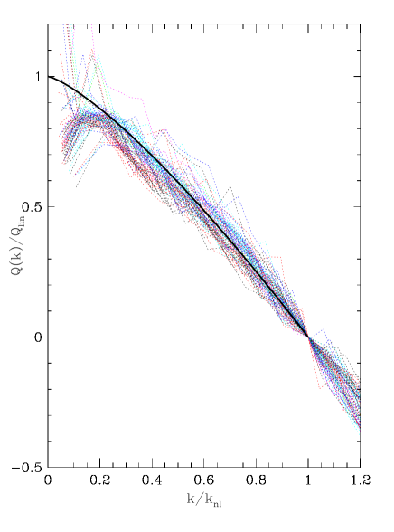
Figure 2: The scaled quadrupole-to-monopole ratio for all the simulations and bias models described in CHWF. The $y$-axis is scaled to the expected, linear theory value of $Q$ (equation 2.1), the $x$-axis is scaled to the zero-crossing scale of the quadrupole, $k_{\rm nl}$. The thick black line is our empirical fit, equation 2.2.

We expect the redshift-space distortions to tend asymptotically towards linear behaviour on the largest scales. The statistic we use to parametrise the distortions is the quadrupole-to-monopole ratio, $Q(k)\equiv P_{2}(k)/P_{0}(k)$, where $P_{0}(k)$ and $P_{2}(k)$ represent the monopole and quadrupole terms of the 3-dimensional redshift-space galaxy power spectrum $P({\bf k})$. In the linear regime, a positive value of $Q(k)$ is produced by coherent infall onto overdense regions and outflow from underdense regions. The distortion, computed first by Kaiser [Kaiser (1987)], depends only on $\beta$ and the resulting expression for the quadrupole-to-monopole ratio is

$$Q_{\rm lin}=\frac{4\beta/3+4\beta^{2}/7}{1+2\beta/3+\beta^{2}/5}$$ (2.1)

(eg. [Cole et al. (1994)]). Most physical models of local galaxy bias result in a bias function, $b$, that, despite being scale dependent on small scales, tends to a constant value on large scales [Coles (1993), Mann et al. (1998)]. Thus, $\beta$ itself is expected to be constant in this regime, and, as a starting point, any model of $Q(k)$ should have this asymptotic behaviour on large scales.

On smaller scales the quadrupole-to-monopole ratio is suppressed from its linear value. Eventually, $Q(k)$ becomes negative, where the random motions inside highly non-linear overdense regions produce structures elongated along the redshift direction (fingers of God). Most of the information that can be used to constrain $\beta$ comes from the quasi-linear regime, where $Q(k)$ is suppressed but still positive. We therefore seek a model for $Q(k)$ over just this range of scales.

We measure $Q(k)$ from the simulations using the technique of fast Fourier transforms, presented in HC98. We first simulate redshift-space anisotropy by picking one of the coordinate axes of the simulation as a redshift direction, and perturbing all the particle positions by their velocities in this direction. As noted in HC98, using a single line of sight for the simulation ensures that the distant observer approximation holds, by effectively placing the simulation at an infinite distance. The galaxy density field, $\delta({\bf r})$, is Fourier transformed to obtain $\delta({\bf k})$, and $\hat{P}({\bf k})\equiv\langle\delta({\bf k})^{2}\rangle$ is taken as the estimate of the power spectrum at each grid point in $k$-space. This three-dimensional, anisotropic power spectrum is then decomposed into spherical harmonics to obtain the monopole (or spherically averaged power), $P_{0}(k)$, and quadrupole, $P_{2}(k)$.

Fig. 2 shows the quadrupole-to-monopole ratio, $Q(k)\equiv P_{2}(k)/P_{0}(k)$, for all the galaxy distributions resulting from each cosmological model and local biasing prescription investigated in CHWF. We have scaled the curves such that the $x$-axis is measured in units of the wavenumber, $k_{\rm nl}$, where the quadrupole crosses zero, and the $y$-axis is scaled by the expected, linear theory value given by equation 2.1.

At low $k$, there is substantial scatter between the curves, and a turn down from the linear value in the first two bins. This feature was explained in CHWF as resulting from a random down-turn in power on these scales in the simulations we used: the majority of the simulations are based on the same initial random phases, so this down-turn is repeated in all the simulations.

Apart from this trend, it can clearly be seen that the curves generally have a common locus once they have been scaled in this way. It is thus reasonable to seek a model for $Q(k)$ of the form $Q(k)=Q_{\rm lin}f(k/k_{\rm nl})$. A good empirical fit of this form is provided by

$$f(x)=1-x^{1.22},$$ (2.2)

which is shown by the heavy solid line in Fig. 2.

We have thus found a model with two free parameters, $\beta$ and $k_{\rm nl}$, which accurately describes the shape of the quadrupole-to-monopole ratio, $Q(k)$, for the wide range of models considered in CHWF.

This is rather similar to the approach used by ?) who fit an empirical curve to their analytic Zel’dovich approximations for the quadrupole using the same scalings. We stress that our approach should be far more general since it is based on the fully non-linear data provided by N-body simulations, covers a much broader range of cosmologies, and includes the effects of bias.

2.1 Definition of bias

Figure 4: Scatter plots for two realizations of the $\Omega_{0}=1$, $\tau$CDM, simulations (named E3SA and E3SB in CHWF), biased with each of the six biasing prescriptions described in CHWF. The point types reflect different bias models: model 1 (stars), 2 (crosses), 3 (circles), 4 (open squares), 5 (solid triangles), 6 (open triangles). On the left we show comparisons of the fit $\beta$ with the input $\beta=\Omega^{0.6}/b$, where the bias factor, $b$, is defined by the ratio of the fluctuations in spheres of radius $8h^{-1}\,{\rm Mpc}$ in the galaxy and matter distributions. On the right, the bias factor is instead defined on a larger scale, as the ratio of fluctuations in spheres of radius $20h^{-1}\,{\rm Mpc}$.

The conventional method for specifying the bias factor, $b$, is by the ratio of rms fluctuations in spheres of radius $8h^{-1}\,{\rm Mpc}$ in the galaxy density to those in the mass density. In the approximation that both power spectra have the same shape, or at least the same shape on scales that contribute to the fluctuations in $8h^{-1}\,{\rm Mpc}$ spheres, this is equivalent to a boost in the galaxy power spectrum normalization by a factor $b^{2}$ relative to the mass spectrum. Most physical prescriptions for galaxy formation, in contrast, result in a bias that is to some extent scale dependent [Mann et al. (1998), Benson et al. (1999b), Blanton et al. (1999)]. For example, the large-scale galaxy distribution may have a constant bias, but this may be reduced in clusters where the number density is sufficiently high that a significant amount of merging has occurred.

In Fig. 4 we show the result of fitting our empirical model to the two simulations for which the widest range of biasing schemes is available. These $\tau$CDM simulations (named E3SA and E3SB in CHWF) have been biased using all six prescriptions described in CHWF. The left hand panels show the scatter of $\beta_{\rm fit}$ versus $\beta_{8}=\Omega_{0}^{0.6}/b_{8}$. The diagonal line represents the ideal, one-to-one correspondence between the estimated and true values of $\beta$. The labels at the bottom of each panel give the average difference between the fitted and true values, and also the scatter around the mean relation. As can be seen, for any one simulation, most of the biasing prescriptions result in the same values of $\beta_{8}$; not really surprising, since most of them were fixed to reproduce clustering on these scales. Different prescriptions for biasing the galaxy catalogues, however, result in systematically different best-fitting values of $\beta$, despite the constraint that $\beta_{8}$ is the same. This produces significant scatter in the values of $\beta_{\rm fit}$ for these different biases.

In contrast, the scatter is much reduced in the right hand panels in which we plot $\beta_{\rm fit}$ against $\beta_{20}$, where $\beta_{20}$ is obtained using the bias factor, $b_{20}$, defined by the ratio of galaxy to mass fluctuations in spheres of radius $20h^{-1}\,{\rm Mpc}$. Ideally we would like to define the bias parameter on very large scales which would truly reflect the asymptotic value of the bias, but in practice the finite volume of the simulations makes estimates of the bias on such scales rather noisy. CHWF presented a method for calculating analytically the asymptotic value of the bias, but this method can only be applied to the subset of bias models that are based on the initial linear density field rather than the evolved non-linear density field. We expect $b_{20}$ to be a good approximation to the asymptotic large scale bias in all cases.

Use of $\beta_{20}$ rather than $\beta_{8}$ has a dramatic effect on the scatter of the different models, pulling them much closer to the $\beta=\beta_{\rm fit}$ line. The scatter is reduced by a factor of four in these models. This tighter correlation indicates that the quadrupole, despite being measured over a range of mostly quasi-linear wavenumbers, constrains quite directly the large-scale linear bias factor.

2.2 Comparison with existing models

We now compare our two-parameter model for $Q(k)$ with the analytic velocity dispersion models which are commonly used in the analysis of redshift-space distortions. In fact, three models of velocity dispersion have generally been considered in the literature:

1. Gaussian. Particle velocities are drawn from the distribution ${\mathcal{P}}(v)\propto\exp(-v^{2}/2\sigma_{v}^{2})$. In this case the convolution in real space results in a multiplication of $\delta({\bf k})$ by the factor $\exp(-k^{2}\mu^{2}\sigma_{v}^{2}/2)$, where $\mu$ is the cosine of the angle between the wave-vector, ${\bf k}$, and the line of sight.

2. Exponential. The particle velocities have ${\mathcal{P}}(v)\propto\exp(-\sqrt{2}|v|/\sigma_{v})$. Then, $\delta({\bf k})$ is multiplied by $(1+k^{2}\mu^{2}\sigma_{v}^{2}/2)^{-1}$.

3. Pairwise exponential. In this case, the pairwise velocity dispersion of the particles is assumed to come from an exponential distribution like that of the exponential model. The multiplicative factor is the square root of that in the previous case, and so the power spectrum itself ($|\delta({\bf k})|^{2}$) is multiplied by $(1+k^{2}\mu^{2}\sigma_{v}^{2}/2)^{-1}$.

The value of $\sigma_{v}$ that appears in the pairwise formula is the pairwise velocity dispersion, equal to $\sqrt{2}$ times the point-wise dispersion. Thus, if we Taylor expand each of the three factors, we find that the first order term is the same in each case; the distributions have the same width, but different shapes.

As pointed out by ?), this effect cannot be considered in isolation; the linear Kaiser boost to the power spectrum also contains terms in $\mu$, and so to extract the harmonic moments, $P_{0}(k)$ and $P_{2}(k)$, one must first multiply these two factors together before weighting by the appropriate Legendre polynomial and averaging over the line-of-sight angle. We use the maple computer package to perform these calculations. In Fig. 6 we compare the three different velocity dispersion model predictions for the shape of $Q(k)$ with the shape we obtain for our empirical model, which we know (from Fig. 2) is a reasonable fit to the simulations. It is clear that the shapes of the velocity dispersion models do not match that of the empirical model, and that these models always underestimate the level of deviation from the linear theory result on large scales. This breakdown is due to the violation of the assumption that non-linear behaviour arises purely through thermal motions in virialized systems at a fixed velocity dispersion. In fact, the velocity dispersion will be correlated with the density field, and coherent non-linear flows may play an important part at large scales.

Figure 6: Comparison of our empirical model for $Q(k)$ with results from a Gaussian, exponential, and pairwise exponential model. These models were computed for $\beta=0.55$ and a one-dimensional point-wise velocity dispersion of $400{\rm km\,s^{-1}}$.

It is clear that using the velocity dispersion models to measure $\beta$ will result in some degree of bias, since the curves are not a good fit to the N-body data. In order to assess the significance of this bias we use the FFT method of estimating the redshift-space power spectrum and its quadrupole-to-monopole ratio from the simulation cubes, as outlined above and described in HC98, for the full set of simulations described in CHWF.

In Fig. 8 we show a scatter plot for the behaviour of $\beta_{\rm fit}$ with the known value of $\beta_{20}$, as defined above. Each panel is labelled with the dispersion model used to make the fit, and the figure includes every biasing scheme of every cosmological model presented in CHWF. It is immediately clear from this figure that the velocity dispersion models all produce a systematic offset between the fitted and true values of $\beta$. The pairwise exponential model comes closest to fitting the data, but this still results in a systematic underestimate of $\beta$ by $\approx 0.1$. Judging from a number of recent results (for a summary, see table 1 of [Hamilton (1998)]), we expect to find $\beta\sim 0.5$, so this represents a $20\%$ bias in measuring $\beta$, certainly rather larger than the random errors expected from large surveys like 2dF and SDSS. The estimator based on our empirical model, shown in the bottom right-hand panel, has similar scatter to the other estimators but there is no appreciable systematic offset over a wide range of $\beta$. The only regime where the model appears to break down is for $\beta\mathrel{\hbox{\hbox to0.0pt{\hbox{\lower 4.0pt\hbox{$\sim$}}\hss}\hbox{$<$}}}0.3$, which is at the very low end of the range allowed by current observations.

Figure 8: Scatter plots of $\beta_{\rm fit}$ for a sample of over one hundred simulations. Each panel shows the results of using a different redshift-space distortion model to extract the value of $\beta_{\rm fit}$, as indicated by the name in the top left corner. We also quantify the systematic offset, $\langle\beta-\beta_{\rm true}\rangle$, and the scatter, $\sigma$, about the mean value.

2.3 Intrinsic scatter

In addition to the original two $\tau$CDM simulations (E3SA and E3SB of CHWF), we now have a further eight simulations of the same cosmological model. All ten of these realizations have been biased with one of the bias prescriptions. The scatter in the resultant $\beta_{\rm fit}$ values of $\sigma=0.03$ is an indication of the limiting accuracy to which $\beta$ can be determined due to the finite volume of these simulations. This result indicates that the offsets in $\langle\beta-\beta_{\rm true}\rangle$ seen for the empirical model fits in Figs. 4 and 8 are statistically insignificant.

3 Analysis of redshift surveys

Having demonstrated that our empirical model for the quadrupole $Q(k)$ can be used to make essentially unbiased estimates of the redshift-space distortion parameter $\beta$, we now turn to the question of how accurately $\beta$ can be measured from a real galaxy redshift survey. We choose to apply the technique to the geometry of the 2dF South Galactic slice [Colless (1995)].

First, in section 3.1, we address this question by making use of mock galaxy catalogues drawn from the ten independent biased $\tau$CDM N-body simulations mentioned above. Then, in section 3.2, we perform a similar analysis of idealized mock catalogues, in which the galaxy density field is assumed to be a Gaussian random field. The results are compared in section 3.3.

3.1 N-body mock catalogues

The ten mock 2dF galaxy catalogues that we analyse here have many realistic features. They are based on N-body simulations in which the small scale structure has been accurately evolved into the non-linear regime. The galaxies are biased tracers of the underlying dark matter, and have a correlation function that, on small scales, matches that of the galaxies in the APM survey. The 2dF South Galactic slice is approximately $90\hbox{${}^{\circ}$}$ long in right ascension, with declination range $15\hbox{${}^{\circ}$}$ centred on $\delta=30\hbox{${}^{\circ}$}$. Our mock catalogues have the same geometry on the sky, and are constructed with a similar radial selection function to that expected from the real survey. The way in which we deal with the wide opening angle of the survey and select the galaxy sample to analyse is outlined below.

3.1.1 Distant observer approximation

The Cartesian linear-theory formalism of ?) is applicable only when the line-of-sight direction is constant across the whole survey. In this case, when the redshift-space density field is decomposed into the sum of plane waves, only the components of the waves parallel to the line of sight are affected by the redshift-space distortion [Zaroubi & Hoffman (1996)]. Thus it is not directly applicable when the galaxy survey subtends a large angle on the sky. Whilst there do exist methods of dealing with wide angle surveys in one go, by expanding the density field into spherical harmonics [Heavens & Taylor (1995)], we do not concern ourselves with those here. Rather, we split the survey up into separate angular bins with relatively small opening angle, and treat each one with the plane parallel approximation. For the 2dF SGP geometry, the declination range is $15\hbox{${}^{\circ}$}$. It thus seems reasonable to pick a right ascension range for the angular bins of comparable extent. The width of the South Galactic strip is $\approx 90\hbox{${}^{\circ}$}\cos 30\hbox{${}^{\circ}$}=78\hbox{${}^{\circ}$}$. We split the survey into three bins each spanning $26\hbox{${}^{\circ}$}$ in right ascension. Note that there are pairs of galaxies that span adjacent bins but still have opening angle less than the $26\hbox{${}^{\circ}$}$ bin width. To avoid throwing this data away, we also include the two overlapping bins. The effect of a finite opening angle on the estimated value of $\beta$ has been studied by ?). From their fig. 8 it is clear that a $26\hbox{${}^{\circ}$}$ opening angle should only result in a one per cent underestimate of the quadrupole-to-monopole ratio of the power spectrum. Since $Q_{\rm lin}(\beta)$ is, from equation 2.1, approximately linear over a reasonable range of $\beta$ (estimates of $\beta$ range from around $0.2$ to $1.0$ [Hamilton (1998)]), this introduces only a minor systematic error. We thus perform the analysis for five bins of angular extent $\approx 26\hbox{${}^{\circ}$}\times 15\hbox{${}^{\circ}$}$ and average the resulting power spectrum estimates.

3.1.2 Volume limited samples

The great advantage of surveys with such depth and sampling as 2dF and SDSS is the ability to construct volume limited samples of galaxies. We can thus look at the clustering properties of a particular class of galaxies, avoiding the problems that arise if bias is a function of luminosity.

In a volume limited sample, we throw away all the galaxies beyond a certain redshift limit, and all galaxies with absolute luminosities such that they would not make it into the catalogue if they were located at that redshift limit.

For the genuine survey it will be interesting to carry out analysis of redshift-space distortions for a set of volume limited catalogues of varying depth. Here we simply illustrate the analysis for one volume limit chosen to be close to optimal for determining $\beta$. As the volume limit is increased we retain only the brighter galaxies, and so the galaxy number density decreases and the shot-noise contribution to the power spectrum increases. For an accurate constraint on $\beta$, we should choose a depth for which the survey will give reliable data, without errors due to shot noise dominating over the contribution due to the finite size of the survey volume. For the purposes of illustration, we have chosen this depth to be such that the resulting shot-noise contribution to the power spectrum is equal to that of the clustered galaxy distribution at $k=0.3h\,{\rm Mpc^{-1}}$, so that on larger scales the error on $P(k)$ is not shot-noise dominated. The reason for this choice of scale is simply that we are going to fit our model for the quadrupole distortion only as far as the zero-crossing scale $k_{\rm nl}$, which, for the model under investigation, is $k_{\rm nl}\approx 0.3h\,{\rm Mpc^{-1}}$. The resulting redshift limit arising from this procedure is $z\approx 0.29$. The median redshift of the survey is rather lower than this, $\bar{z}\approx 0.1$.

At this limit, the survey is very sparse, with ${\bar{n}}\approx 5\times 10^{-4}h^{3}\,{\rm Mpc^{-3}}$. We stress that this sacrifice in density has been made in order to probe the longest, most linear scales as accurately as possible, and that the resultant high shot noise has little or no detrimental effect on measurements of the long wavelength, high amplitude modes.

In catalogues with this depth, we expose ourselves to a number of factors which can contaminate the clustering signal. The ten mock catalogues considered here are constructed from simulations with $\Omega_{0}=1,\Lambda_{0}=0$. In general, the mapping from redshift to comoving distance is a function of the cosmology, and so, if the wrong cosmology is assumed in this transformation, the size of a volume element will appear to change with redshift, essentially mixing the measured clustering between scales. This effect is only expected to be noticeable for high redshift samples, $z\mathrel{\hbox{\hbox to0.0pt{\hbox{\lower 4.0pt\hbox{$\sim$}}\hss}\hbox{$>$}}}0.1$, and so a sample of this depth would require investigation to determine the magnitude of potential bias given the uncertainty in cosmology. Inherent in having a significant look-back time is the possibility for significant evolutionary effects within the sample. As the density field evolves under gravitational instability, the strength of clustering increases. Conversely, if the galaxies are biased tracers of the density field, the bias factor approaches unity as evolution progresses [Fry (1996)], so the resultant effect on galaxy clustering is quite non-trivial to compute. Furthermore, we should allow for the possibility that the galaxies can themselves evolve, so a sample of galaxies between certain luminosity bounds at high redshift will not necessarily have the same clustering properties as a similar sample in the local Universe.

The interplay between these factors is complex, and we make no attempt to deal with any of these effects here, assuming that they are either insignificant, or that they can be accurately corrected for in real datasets. In section 5 we will discuss the increase in accuracy that comes about if we deal with the whole, magnitude limited catalogue rather than a volume limited subsample.

3.1.3 Estimates of $\beta$

In order to estimate $\beta$ for each mock catalogue we first estimate the power spectrum and $Q(k)$ for each catalogue using a standard FFT method. To perform the fit we also need an estimate of the error on each measurement of $Q(k)$ and ideally the covariance of the estimates of $Q(k)$ at different values of $k$. These covariances arise through the finite size of the window function, and we estimate the full covariance matrix introduced by this effect using the method of multiple idealized mock catalogues that will be described in the following section. We then use this matrix to make generalised minimum-$\chi^{2}$ fits of the empirical model of $Q(k)$ to each of the ten realizations. This process results in an estimate of $\beta$ for each of the mock catalogues.

The true value of $\beta$ in these simulations is (the stars in Fig. 4) $\beta_{\rm true}=\beta_{20}=0.55$, while from the mock catalogues we find an average value of $\beta_{\rm av}=0.493$, with a scatter of $\sigma=0.173$. First we note that the difference between $\beta_{\rm true}$ and $\beta_{\rm av}$ is not statistically significant given that the standard error on the mean of the ten realizations is $0.173/\sqrt{10}=0.055$. The scatter on $\beta$, however, is around $35\%$ of the mean; this is far in excess of the uncertainty we hope to achieve with a survey of the size of 2dF.

3.2 Idealized linear mock catalogues

We wish to isolate the reason why the scatter in the estimated $\beta$ values is substantially larger than expected. To do this we have generated a large set of idealized mock catalogues in which the galaxy density is explicitly assumed to be a Gaussian random field rather than the result of biasing an evolved N-body simulation.

We construct the density field on a cubic grid by first obtaining its Fourier transform, using a simple model for the redshift-space power spectrum $P^{S}(k,\mu)$ and random phases. We choose one axis to be the line-of-sight direction and so assume that it is constant across the whole survey. This means we avoid the problem of large opening-angle discussed in section 3.1.1, and if we wish we can analyse the whole survey volume in one piece rather than having to slice it into five wedges of smaller opening angle. The difference in accuracy between these two approaches indicates the scope for improving the estimates of $\beta$ by carrying out the analysis using spherical harmonics, which in principle allow the effects of a large opening angle to be treated precisely.

The redshift-space power spectrum we adopt can be expressed as

$$P^{s}(k,\mu)=P_{L}(k)K(\mu)E(k,\mu)+P_{\rm shot}.$$ (3.3)

Here $P_{L}(k)$ is the isotropic real space power spectrum which we assume to be given by the CDM power spectrum of ?):

$$P_{L}(k)\propto\frac{k^{n}\times[\ln(1+2.34q)/2.34q]^{2}}{[1+3.89q+(16.1q)^{2}+(5.46q)^{3}+(6.71q)^{4}]^{1/2}},$$ (3.4)

where $q=k/\Gamma$. As with the galaxy power spectrum of the N-body catalogues we set $n=1$, $\Gamma=0.25$, as suggested by observations of large-scale structure [Peacock & Dodds (1994)] and fix the amplitude such that $\sigma_{8}=0.96$, the value determined for galaxies in the APM survey [Maddox et al. (1996)]. The second factor, $K(\mu)=(1+\beta\mu^{2})^{2}$, is the linear theory redshift-space distortion of ?). The effect of small scale velocity dispersion is modelled using the pairwise exponential dispersion model by setting $E(k,\mu)=[1+(k\sigma_{v}\mu)^{2}/2]^{-1}$ with $\sigma_{v}=500{\rm km\,s^{-1}}$. This is the dispersion model that comes closest to fitting the shape of $Q(k)$ in the N-body catalogues and the value of $\sigma_{v}$ adopted produces a zero-crossing of $Q(k)$ at close to the $k_{\rm nl}\approx 0.3h\,{\rm Mpc^{-1}}$ found in those catalogues. The final term in equation 3.3 represents the shot noise in the catalogue and we set $P_{\rm shot}=1/{\bar{n}}$, where ${\bar{n}}$ is the galaxy number density in the volume limited catalogues of section 3.1.

This model ensures that the power spectrum of these idealized galaxy density fields matches well those of the volume limited N-body mock catalogues analysed above. We now give each mode a random complex phase and use an FFT to produce the galaxy density field in a cube. This field is then sampled using the survey window function. We can then either split this volume into five wedges or analyse the whole volume in one piece. We can also vary the size of the cube in which the density field is constructed to assess how this effects the constraint on $\beta$.

3.2.1 The survey window function

The effect of sampling the galaxy density field only inside certain angular boundaries and with a particular radial selection function can be modelled by multiplying the full galaxy density field, $\delta({\bf r})$, by a spatial window function, $W({\bf r})$. The effect on the Fourier transform of the density field is that of a convolution with the transform $W({\bf k})$, and similarly the power spectrum is convolved with $|W({\bf k})|^{2}$. This process can be thought of as a smoothing of the three-dimensional power spectrum, $P({\bf k})$, with an anisotropic window function $|W({\bf k})|^{2}$. On large scales (small $k$) the effect of this is to suppress the quadrupole-to-monopole ratio. In fitting our models to the $Q(k)$ measured from the mock surveys we take account of this by first explicitly convolving the model power spectrum with the survey window function. We do this numerically using FFTs and the convolution theorem.

3.2.2 Estimates of $\beta$

As with the N-body mock catalogues we estimate $Q(k)$ for each realization of an ensemble of mock catalogues. Here we can use many more than ten and so determine the mean, variance and covariance of the values of $Q(k)$ very accurately. We use the resultant covariance matrix to perform a fit to $Q(k)$ in each realization over the same range of $k$. In this case the model for $Q(k)$ that we fit is that for the analytic pairwise exponential model that we used to construct the power spectra. Thus we are again in the idealized realm of having a completely accurate model for the redshift-space distortions, but we have shown that the empirical model is indeed a good fit to the N-body simulation data. Both models for $Q(k)$ have two parameters which control the large-scale asymptote and the zero-crossing, so it is reasonable to assume that confidence limits on $\beta$ derived using one model will be similar to those using the other.

The resulting scatter in $\beta$ when we analyse the idealized mock catalogues split into the five wedges as we did for the N-body mock catalogues is $20\%$. This result is almost a factor of two smaller than the scatter we found in section 3.1.3.

If we analyse the whole survey coherently, without splitting it up to satisfy the distant observer approximation, then we find a scatter of $16\%$. This change from $20\%$ to $16\%$ represents the modest improvement that can be made if one accurately deals with the complications of the effects of the large opening angle of the 2dF survey.

The effect of increasing the simulation box size to the point where it is much larger than that used for the N-body simulations and much larger than the depth of the 2dF survey is to reduce the scatter from $20\%$ to $18\%$. Thus little information is lost due to the finite volume of the N-body simulations used to create the mock catalogues.

3.3 Discrepancy

We now address the question of why the mock catalogues based on the N-body simulations produced an error on the estimated value of $\beta$ almost twice as large as the idealized analysis predicts.

Fig. 10 shows the fractional error on $P(k)$ and the absolute error on $Q(k)$ as a function of wavenumber. It compares the variance from the ten independent N-body mock catalogues with the error we find from the idealized Gaussian random fields. The correspondence between the two error estimates clearly indicates that the Gaussian random field method has not under-predicted the degree of uncertainty on the distortion of each individual mode. We also note that these error estimates are in good agreement with the values predicted by the method of error analysis detailed in [Feldman et al. (1994)]. We therefore conclude that the reason for the difference in the errors in $\beta$ must be due to the existence of significant correlations between $Q(k)$ at different values of $k$. These correlations are over and above those that are induced by the shape of the survey window function, which we have taken into account in both methods. Therefore they must be a result of non-linear gravitational evolution and so cannot be modelled by a Gaussian density field.

Gravitational instability on small scales causes coupling between different modes of the density field, resulting in correlations between the phases of these modes [Meiksin & White (1999)]. We fail to take into account this non-linear effect when using idealized, linear mocks, but it is implicit in the N-body method which has followed the evolution of these modes accurately. We only expect linear theory to be valid for $\Delta^{2}(k)\ll 1$, where $\Delta^{2}(k)=4\pi/(2\pi)^{3}k^{3}P(k)$, and this condition is certainly not met in our N-body simulations around the zero-crossing of the quadrupole. However, the strength of the effect is perhaps initially surprising.

Figure 10: The fractional error on the power spectrum (upper panel) and absolute error on the quadrupole-to-monopole ratio (lower panel). The solid line is from the variance between then ten independent N-body mock catalogue realizations of the survey, the dotted line is from one hundred ‘linear’ mocks as described in section 3.2. We have attached Poisson error bars to the points using the relation that the standard deviation of the scatter is given by $\sigma_{\rm ss}=\sigma_{\rm s}/\sqrt{2(N-1)}$, where $\sigma_{\rm s}$ is the measured scatter from $N$ realizations [Barlow (1989)].

As a first attempt to deal with these non-linearities, we repeat the N-body fits described in section 3.1.3, but replace the covariance matrix used previously with a new matrix that is obtained from the ten realizations themselves. The off-diagonal terms in this matrix arise from mode coupling caused by the survey window function and also non-linear evolution of the density field. The error in the estimate is now reduced from $35\%$ to $25\%$. This reduction occurs because previously we attached much weight to the quasi-linear regime, to modes at intermediate wavelengths close to, but longer than, $k_{\rm nl}$, where the quality of data appeared good. In actual fact, this regime is also the scene of strong non-linear mode coupling, so the data are not in fact as good as previously believed. Applying the more realistic weighting scheme makes better use of the data, and hence produces less scatter in the estimate of $\beta$. Unfortunately, this method of obtaining the covariance matrix is time-consuming, since it involves producing multiple large-volume N-body simulations for each cosmology and power spectrum that is to be studied.

3.4 Summary

In sections 2 and 3, we have:

• used biased N-body simulations to develop an accurate, empirical model for $Q(k)$.

• used mock catalogues drawn from these simulations to illustrate how accurately $\beta$ can be measured in practice.

• used linear mock catalogues to show how much of the uncertainty in $\beta$ comes from just the finite volume effect.

• demonstrated that, in fact, a major source of random error is the coupling of non-linear modes.

• shown that allowing for this coupling (by using a covariance matrix derived from the full mock catalogues, rather than the linear mocks) results in a large improvement in constraining $\beta$.

The error has been reduced by allowing for non-linear effects, but is still rather large, in excess of the level of constraint that could be achieved if non-linearities were not present at all. In the next section, we outline a practical method for reducing the non-linearities and thus increasing the accuracy of the estimates. It is also worth mentioning the approach adopted by ?), who finds a method for constructing a near minimum variance estimator for the non-linear power spectrum based on assembling a set of almost uncorrelated non-linear modes. The use of such optimal methods in both the non-linear and linear regimes may provide the capability to constrain $\beta$ rather better than we do in this work, although the methods are still in the development stage and it is not clear how easily they can be applied to a real dataset.

4 Collapsing clusters

In the dispersion models one assumes that the random velocities induced by non-linearities are uniform and uncorrelated with the density field. In reality we do not expect this to be the case; the coupling between $k$-modes is a local effect in $r$-space, taking place inside particular non-linear structures. In these volumes, mode coupling is extremely strong. As pointed out in HC98, if we can somehow excise these regions from our treatment, we could create a better behaved, more linear quadrupole-to-monopole ratio. In addition, this would have an even more dramatic effect in lessening the correlations between modes on these scales. This result could be achieved by identifying and removing the signal from clusters, as described in HC98.

Here we illustrate the application of this method. Taking the ten simulations used earlier, we identify clusters in real space using a friends-of-friends [Davis et al. (1985)] algorithm with linking length $0.2$ times the mean inter-particle separation. We select clusters with ten or more members, and compute the mean velocity of each cluster by averaging over the velocities of its members. The cluster members then have their velocities in the simulation replaced with that of their parent cluster. In this way, it was shown in HC98, the effect of non-linear velocity dispersions can be heavily damped.

In a real survey, clusters will have to be measured without the perfect knowledge of galaxy density field which we have assumed here, and in redshift space rather than real space. This is likely to involve a number of parameters and considerations, and from this point of view it seems pointless to develop an accurate model for the cluster-collapsed $Q(k)$ since this will not be generally applicable. Here we instead take as a model for $Q(k)$ the shape measured from averaging the ten full-cube simulations. We multiply this by a single free parameter, $Q_{\rm lin}$, which we assume is related to $\beta$ via the linear theory result (equation 2.1). For the set of $\tau$CDM simulations, non-linearities are suppressed to the extent that the quadrupole now crosses the $k$-axis at $k_{\rm nl}=0.8h\,{\rm Mpc^{-1}}$.

Having derived this model from the simulations, we now apply it to mock catalogues. These are created from the cluster-collapsed simulations, with the same parameters and selection functions as the mock 2dF SGP catalogues used in section 3. We then apply the same FFT technique explained above to measure $Q(k)$ in the mock catalogues.

We perform the fits over the same range of $k$ as before ($0<k<0.3h\,{\rm Mpc^{-1}}$), using a covariance matrix obtained from the ten independent cluster-collapsed mock catalogues. We find that the scatter in $\beta$ is reduced from $25\%$ to $13\%$. This is better than the result from the Gaussian random fields and indicates that collapsing clusters has successfully removed most of the mode correlations on these scales. Collapsing the clusters has pushed the zero-crossing of $Q(k)$ to smaller scales, so we may be able to reduce the uncertainty still further by extending the range over which we fit the model. However, this is not the case; extending the fits to $k=0.6h\,{\rm Mpc^{-1}}$ results in no significant increase in accuracy. This is because the data in this range is much noisier than in the uncollapsed case, aiding little in fitting the the curve.

We note that now we are using scales that were previously quasi-linear to determine $\beta$, so the fits will not be greatly improved by relaxing the small angle constraint. Much of the new data is coming from pairs whose separation on the sky is small compared to the full extent of the survey.

5 A magnitude limited sample

Throughout the above work we have used the same volume limited sample with $z_{\rm lim}=0.29$ to measure $\beta$. Volume limiting selects a subsample of galaxies, which can be very useful for studying clustering behaviour as a function of luminosity, but at the expense of discarding the majority of galaxies and hence severely reducing the number density of objects. If we are interested in using the survey to measure $\beta$ as well as possible for all the galaxies in the catalogue, we can extend the treatment to the magnitude limited case. For the case of a real survey, this must be done with caution, since we know that galaxies of different luminosity exhibit different clustering properties (eg. [Loveday et al. (1999)]). In our mock catalogues, however, there is no dependence of clustering strength on galaxy luminosity, so any sample should measure the same power spectrum and hence the same $\beta$. A magnitude limited sample will be more accurate since the number of galaxies is higher, and it includes galaxies at higher redshifts, probing more long-wavelength modes. We weight galaxies using the scheme introduced by ?):

$$w({\bf r})=\frac{1}{1+{\bar{n}}({\bf r})P_{\rm w}}$$ (5.5)

where ${\bar{n}}({\bf r})$ is the number density at position ${\bf r}$, and we set $P_{\rm w}=5000h^{3}\,{\rm Mpc^{-3}}$, roughly reflecting the value of the galaxy power spectrum around the middle of the range over which the fit is performed ($k\approx 0.15h\,{\rm Mpc^{-1}}$). This weighting is designed to minimize the variance in estimates of $P(k)$ where $P(k)\sim P_{\rm w}$.

Using this method, applied to the cluster-collapsed catalogues described in the previous section, results in a reduction of the error on $\beta$ from $13\%$ to $10\%$. A similar improvement is expected for the uncollapsed case.

6 Conclusions

There are four distinct results presented in this paper:

1. We have found an empirical model for the quadrupole moment, $Q(k)$, of the redshift-space power spectrum which matches the behaviour of this quantity in a wide range of cosmological models much more accurately than existing analytic models. We have demonstrated that it can be successfully used to obtain unbiased estimates of the redshift-space distortion parameter $\beta=\Omega^{0.6}/b$.

2. We have shown that the resultant measurement of $\beta$ is better correlated with the large-scale bias factor than the usual quasi-linear measure from spheres of radius $8h^{-1}\,{\rm Mpc}$. The quadrupole is thus not sensitive to small-scale scale-dependence of the bias.

3. We have demonstrated that mode coupling caused by non-linear gravitational evolution causes strong correlations between the measured values of $Q(k)$ at different values of $k$, even on quite large scales. This implies that estimates of the accuracy to which $\beta$ can be constrained that are based on assuming the galaxy density field is Gaussian significantly under estimate this error.

4. The most non-linear regions of the density field are galaxy clusters. Although these are compact structures in real-space they are very extended in redshift space and so can affect quite large scale modes in the redshift-space density field. We have shown that by identifying and collapsing galaxy clusters we are broadly successful at both reducing the correlation and increasing the range of scales over which $Q(k)$ can be reliably fitted.

For a set of 2dF southern slice mock catalogues which have a true value of $\beta=0.55$, our empirical model of redshift space distortion produces unbiased estimates of $\beta$ with a $25\%$ statistical error when measured from a volume limited sample with limiting redshift $z_{\rm lim}=0.29$. This model is applicable to the raw, redshift-space galaxy distribution and does not require the identification or manipulation of galaxy clusters. We estimate the statistical error will be significantly reduced (to around $20\%$) if the survey is analysed in one piece, rather than being chopped into five overlapping wedges, which we do in order to satisfy a small angle constraint.

If clusters can be successfully identified and collapsed in the 2dF galaxy redshift survey, analysis of the main southern slice should constrain $\beta$ to a greater accuracy of $13\%$ (volume limited) and $10\%$ (magnitude limited). This error is not expected to be significantly reduced by relaxing the constraint of the distant observer approximation and using galaxy pairs at large angular separation, since much more of the information now comes from pairs that are physically nearer each other, and hence closer together on the sky.

It is worthwhile noting that N-body simulations, when normalized to replicate the observed abundance of galaxy clusters, produce pairwise dark-matter velocity dispersions which are significantly higher than those measured for galaxies [Jenkins et al. (1998)]. This problem is largely alleviated in new models which attempt to realistically identify the places where galaxies form, either by numerical N-body hydrodynamic simulation [Jenkins et al. (1999)], or by semi-analytic modelling [Benson et al. (1999a)]. However, the simple bias models used in this paper produce pairwise galaxy velocity dispersions which are close to those of the dark matter and therefore somewhat higher than for observed galaxies. It is to be hoped that this fact alone will render observational datasets somewhat less prone to non-linear effects than we estimate from our simulations, and the $10\%$ statistical error we find may be a little conservative.

The 2dF survey also contains a slice in the northern Galactic hemisphere. This is a little smaller than the southern slice, but measuring $\beta$ from this data and combining it with the southern slice provides an additional constraint. Assuming the errors add in quadrature, the uncertainty is reduced by a factor $\approx 1.25$.

We thus conclude that the quadrupole moment of the redshift-space distortion measured in the 2dF survey will be capable of constraining $\beta$ to an accuracy of $8\%$. This will yield an important constraint on the density parameter $\Omega_{0}$.

References

- Bardeen et al. (1986) Bardeen J., Bond J., Kaiser N., Szalay A., 1986, ApJ, 304, 15
- Barlow (1989) Barlow R. J., 1989, Statistics: a guide to the use of statistical methods in the physical sciences, Manchester physics series. Wiley
- Benson et al. (1999a) Benson A. J., Cole S., Baugh C. M., Frenk C. S., Lacey C. G., 1999a, MNRAS, submitted
- Benson et al. (1999b) Benson A. J., Cole S., Frenk C. S., Baugh C. M., Lacey C. G., 1999b, MNRAS, submitted, astro-ph/9903343
- Blanton et al. (1999) Blanton M., Cen R., Ostriker J., Strauss M., 1999, ApJ, accepted, astro-ph/9807029
- Cole et al. (1994) Cole S., Fisher K. B., Weinberg D. H., 1994, MNRAS, 267, 785
- Cole et al. (1995) Cole S., Fisher K. B., Weinberg D. H., 1995, MNRAS, 275, 515
- Cole et al. (1998) Cole S., Hatton S. J., Weinberg D. H., Frenk C. S., 1998, MNRAS, 300, 945
- Coles (1993) Coles P., 1993, MNRAS, 262, 1065
- Colless (1995) Colless M., 1995, The 2df galaxy redshift survey, http://msowww.anu.edu.au/heron/Colless/colless.html
- Davis et al. (1985) Davis M., Efstathiou G., Frenk C. S., White S. D. M., 1985, ApJ, 292, 371
- Eke et al. (1996) Eke V. R., Cole S., Frenk C. S., 1996, MNRAS, 282, 263
- Feldman et al. (1994) Feldman H. A., Kaiser N., Peacock J. A., 1994, ApJ, 426, 23
- Fisher & Nusser (1996) Fisher K. B., Nusser A., 1996, MNRAS, 279, L1
- Fry (1996) Fry J. N., 1996, ApJ, 461, L65
- Gunn & Weinberg (1995) Gunn J. E., Weinberg D. H., 1995, in Maddox S. J., Aragón-Salamanca A., ed, Wide-Field Spectroscopy and the Distant Universe, Proceedings of the 35th Herstmonceux workshop. Cambridge University Press, Cambridge, p. 3, astro-ph/9412080
- Hamilton (1998) Hamilton A. J. S., 1998, in Hamilton D., ed, The Evolving Universe. Proceedings of the Ringberg workshop, September 1996. Kluwer Academic Publishers, p. 185, astro-ph/9708102
- Hamilton (1999) Hamilton A. J. S., 1999, MNRAS, submitted, astro-ph/9905191
- Hatton & Cole (1998) Hatton S. J., Cole S., 1998, MNRAS, 296, 10
- Heavens & Taylor (1995) Heavens A. F., Taylor A. N., 1995, MNRAS, 275, 483
- Jenkins et al. (1998) Jenkins A. et al., 1998, ApJ, 499, 20, astro-ph/9709010
- Jenkins et al. (1999) Jenkins A. et al., 1999, in Proceedings X Rencontres de Blois: The Birth of Galaxies, astro-ph/9906039
- Kaiser (1987) Kaiser N., 1987, MNRAS, 227, 1
- Loveday et al. (1999) Loveday J., Tresse L., Maddox S., 1999, MNRAS, submitted
- Maddox et al. (1996) Maddox S. J., Efstathiou G., Sutherland W. J., 1996, MNRAS, 283, 1227
- Mann et al. (1998) Mann R. G., Peacock J. A., Heavens A. F., 1998, MNRAS, 293, 209
- Meiksin & White (1999) Meiksin A., White M., 1999, MNRAS, submitted, astro-ph/9812129
- Peacock & Dodds (1994) Peacock J. A., Dodds S. J., 1994, MNRAS, 267, 1020
- White & Bunn (1995) White M., Bunn E. F., 1995, ApJ, 450, 477
- White et al. (1993) White S. D. M., Efstathiou G., Frenk C. S., 1993, MNRAS, 262, 1023
- Zaroubi & Hoffman (1996) Zaroubi S., Hoffman Y., 1996, ApJ, 462, 25