X-ray Spectra of the RIXOS source sample

Abstract

We present results of an extensive study of the X-ray spectral properties of sources detected in the RIXOS survey, which is a large, nearly complete sample of objects detected serendipitously in ROSAT PSPC fields down to a flux limit of $3\times 10^{-14}$ ergs cm^-2 s^-1 (0.5 – 2 keV). We show that for X-ray surveys containing sources with low count rate, such as RIXOS, spectral slopes estimated using simple hardness ratios in the ROSAT band can be biased. Instead we analyse three-colour X-ray data using statistical techniques appropriate to the Poisson regime which removes the effects of this bias. We also show that the use of three-colour data enables some discrimination between thermal and non-thermal spectra. We have then applied this technique to the RIXOS survey to study the spectral properties of the sample.

For the AGN we find an average energy index of $1.05\pm 0.05$ with no evidence for spectral evolution with redshift. Individual AGN are shown to have a range of properties including soft X-ray excesses and intrinsic absorption. Narrow Emission Line Galaxies (NELGs) also seem to fit to a power-law spectrum, which may indicate a non-thermal origin for their X-ray emission. We infer that most of the clusters in the sample have a bremsstrahlung temperature $>3$ keV, although some show evidence for a cooling flow. The stars deviate strongly from a power-law model but fit to a thermal model. Finally, we have analysed the whole RIXOS sample (extending the flux cutoff to the sensitivity threshold of each individual observation) containing 1762 sources to study the relationship between spectral slope and flux. We find that the mean spectral slope of the sources hardens at lower fluxes in agreement with results from other samples. However, a study of the individual sources demonstrates that the majority have relatively soft spectra even at faint flux levels, and the hardening of the mean is caused by the appearance of a population of very hard sources at the lowest fluxes. This has implications for the nature of the soft X-ray background.

1 Introduction

X-ray surveys have proven to be powerful tools in extending our knowledge of a range of object types, from highly luminous AGN to active stars. Surveys of ‘serendipitous’ detections in the fields of view of imaging X-ray instruments, examples of which are the Einstein Medium Sensitivity Survey (EMSS, Gioia et al. 1990) and the EXOSAT High Galactic Latitude Survey (HGLS, Giommi et al. 1991), have provided large samples with which to make detailed statistical studies with relatively well-understood selection biases. With the advent of ROSAT ever more extensive and sensitive surveys are becoming available, ranging from the ROSAT all sky survey which sampled relatively bright source populations, to deep pencil-beam surveys such as those of Hasinger et al. (1993) and Branduardi-Raymont et al. (1994). Other samples have concentrated on serendipitous sources discovered in ROSAT pointed data (e.g. Boyle et al. 1994, Carballo et al. 1996, Boyle et al. 1995).

The spectral properties of such samples can be a crucial element in understanding the nature of the X-ray emission. However, much of the work to date has considered only the broad-band fluxes of survey sources. The subject of this paper is the RIXOS survey of ROSAT field sources which covers a total of 20 deg² of sky and has a high level of optical identification completeness ($\sim$94% over a 15 deg² sub-area) down to a flux level $3\times 10^{-14}$ ergs cm^-2 s^-1. This flux cutoff is set so as to bridge the gap in sensitivity and sky coverage between the ROSAT all-sky survey and the deepest pencil-beam ROSAT surveys. As the flux cutoff of RIXOS is set at a level which is much higher than the sensitivity threshold of the ROSAT observations used, sufficient numbers of X-ray photons have been detected from all RIXOS sources to provide some information about their overall spectral distribution. This paper examines the X-ray spectral properties of the RIXOS sample. Other aspects of the RIXOS survey are covered in Mason et al. (1998), Page et al. (1996), Puchnarewicz et al. (1996,1997), Carrera et al. (1998) and Romero-Colmenero et al. (1998). The paper discussing cluster evolution by Castander et al. (1995) is based on a subset of the RIXOS complete sample.

2 The RIXOS Sample

The X-ray data are taken from the RIXOS sample of objects (Mason et al. 1998) and have been constructed from serendipitous sources discovered in 80 pointed ROSAT PSPC fields. The fields were chosen to have nominal exposure times greater than 8 ksec and to be above a Galactic latitude of 28 degrees. This limit enables us to sample sources at faint fluxes without the problem of identifying them in crowded fields. From each field we have excluded the target of the observation and only consider sources at less than 17 arc minutes off-axis. Such sources have the best positional certainty and are not masked by the detector window support structure. Survey sources are selected in the 0.4 - 2 keV band; the poorer point spread function and increased background due to diffuse Galactic X-ray emission make the detection of X-ray sources more difficult at softer energies.

Full details of the optical imaging and spectroscopy and identification process are given in Mason et al. (1998). Over 82 fields (or 20.3 square degrees) our sample is completely identified down to a flux limit of $8.4\times 10^{-14}$ ergs cm^-2 s^-1 and over 61 fields (or 14.9 square degrees) we have complete identifications down to our target flux limit of $3\times 10^{-14}$ ergs cm^-2 s^-1. This flux limit is well above the detection limit for all our fields, and for many sources gives a reasonable number of observed counts. Table 2 lists all the sources in the RIXOS fields above a flux limit of $3\times 10^{-14}$ ergs cm^-2 s^-1 (0.5 - 2 keV), giving field ID and source ID (for details see Mason et al. 1998) together with the galactic column ($N_{H}$), date of observation and exposure time (column 5). This is the sample with which we are primarily concerned here, and it will be referred to here as RIXOS.

In total the RIXOS sample contains 404 sources, of which 347 have been identified. The identification of the sources has been based largely on the optical spectra, and we have split them into six categories. These are Active Galactic Nuclei (AGN), Narrow Emission Line galaxies (NELGs, which may include Seyfert 2 galaxies, LINERs, and HII region galaxies), isolated galaxies, clusters of galaxies, active stars and dMe stars. Of the 347 identified sources, 16 are so close together that no separate spectra could be extracted for them, their spectra are included in Table 2 as ‘MERG’. Five more sources (one of them unidentified) were in fields 115 and 116 (Mason et al. 1998) for which no public archival X-ray data were available at the time of writing. This leaves us with 327 identified sources with available X-ray data, of which 205 have been classified as AGN, 18 as NELGs, 6 as isolated galaxies, 30 as clusters, 46 as stars and 22 as dMe stars. In addition, we have also fitted the spectra of 56 unidentified sources (included in Table 2 as ‘UNKN’). In total, the RIXOS sample forms the largest serendipitous survey constructed from ROSAT PSPC pointings to date, with a larger sky coverage than comparable samples such as the Cambridge-Cambridge ROSAT Serendipity Survey.

3 Data reduction

From the RIXOS sample we have taken all those sources which have a firm optical identification and have extracted three-colour X-ray data. After the recommendation of Snowden et al. (1993) we have used bands S1 (channels 8-41), H1 (channels 52-90) and H2 (channels 91-201). For each field we have constructed an image in each of the three-colours and have ensured the optimal signal-to-noise by excluding high background times and those times when the attitude solution was bad. In general, this excluded between 5 and 20% of the data. We then extracted the source counts for all the known sources in the field (including those with no identification) using an extraction circle of 54 arc seconds, which includes 90% of the ROSAT PSF and maximises the signal to noise for weak sources. In those cases where there was a contaminating source nearby, the extraction circles were reduced in size until there was no overlap. The sizes of the extraction circles for each source are listed in table 2 (column 6) and the fraction of the PSF included for each source is taken into account during the spectral fitting process (section 5.1).

As we are studying very faint sources, we have been careful to obtain an accurate estimate of the background. After masking out all the sources from an image, it was flattened using the exposure map supplied as part of the standard SASS processing. As the exposure map corrects for vignetting and other instrumental effects, we can obtain an accurate estimate of the image background corrected for systematic instrumental effects by summing over a large number of pixels. For RIXOS we summed the data between 5.2 and 10.8 arc-minutes off-axis thereby excluding the residual effects of any bright central source. We can then estimate the background at any given source position from the mean background using data from the exposure map at the required position. This method yields a very accurate background estimate based on a very large number of pixels compared to the number of pixels in the source extraction circle and to a very good degree of approximation we can then assume that this background estimate has a negligible error. Table 2 lists the the extracted counts for the RIXOS sample (columns 8-10) and the background estimates in each of the three bands (columns 11-13).

4 The Colour-Colour diagram

As a first step in studying the spectral properties of the sources, we have constructed a colour-colour diagram including all identified sources in the RIXOS sample (Figure 1). Our normalised colours are defined as

$$C1=(S-H1)/(S+H1)$$ (1)

and

$$C2=(H2-H1)/(H2+H1).$$ (2)

The first plot in figure 1 shows uncorrected colours, and the second shows colours corrected for the effect of galactic absorbing column where applicable. As the correction for the galactic column is model dependent, we have used a power-law fitted to the three-colours (see section 6), and have only applied the correction to extra-galactic sources. Figure 1 shows a number of features. On average the AGN tend to be softer than most of the other sources when corrected for galactic absorption, though it is clear that not all the AGN are soft and some AGN occupy portions of the diagram appropriate to hard sources (see also Figure 7). Five out of 205 AGN have $C1<0$, implying that they are very hard or intrinsically absorbed. A further 15 sources do not appear on this diagram at all since they were not detected in the soft band, and of these six are identified with AGN. This implies that $\sim 5$% of AGN are very hard and are candidates for intrinsic absorption.

Figure 1: The Colour-Colour diagrams for the RIXOS sample of objects. The top panel shows the data uncorrected for the effect of galactic $N_{H}$, while the bottom panel is corrected for galactic $N_{H}$. Different classes of objects have different symbols ($+$ AGN, $\diamond$ ELG, $\bigtriangleup$ Galaxies, $\Box$ clusters and $\star$ stars (including dMe stars)).

As a first step in categorising the spectral characteristics of our sample, we have quantified the differences between the different types of X-ray sources in the colour-colour plot by using a two-dimensional Kolmogorov-Smirnov test. The method used is taken from Press et al. (1992) and the results are shown in Table 1 for both the un-corrected and corrected colour-colour data. The probabilities quoted are of the two samples being drawn from the same parent distribution. However, many of the sources are faint and therefore have large uncertainties which are not taken into account by a standard KS test. We have quantified the possible effect of the measurement uncertainties on the K-S probabilities. To do this we have simulated 100 samples with the same flux distribution as our real sample but assuming that all sources have power-law slopes distributed in a similar way to the AGN. We have used a mean slope of $\alpha=1$ and a dispersion of 0.55. The numbers in brackets in table 1 are the fraction of the time that a K-S probability was obtained that was smaller than the one seen in the original dataset. This therefore gives an indication of the likelihood of obtaining a probability as small as that seen or better by chance alone given our assumption concerning the distribution of AGN slopes.

The 2-d Kolmogorov-Smirnov test emphasises the fact that on average the AGN and objects classified as Narrow Emission Line Galaxies (NELGs) lie in a region of the colour-colour plot distinct from the clusters and stars. The similarity between the NELGs and the AGN as well as the disparity between the NELGs and the clusters/stars is intriguing and may hint at NELGs containing AGN like activity. If the emission were to arise solely from thermal emission from hot gas, the NELGs may be expected to lie further to the left in the colour-colour diagram, closer to the clusters.

‘

The other sources lie to the left of the AGN in the colour-colour diagram. That the stars and clusters are distinct from the AGN is not surprising, given the different physical mechanism known to underly their X-ray emission. From Figure 1 the stars constitute the hardest sources with the clusters lying midway between the stars and AGN. However, within the stars from Table 1 there is a further difference which would seem to indicate that the dMe stars are softer than other active stars. Given the multi-temperature nature of the emission from stars, simple three-colour data cannot give more than an indication of a difference in the X-ray spectra between these two classes of objects.

Table 1: Two dimensional Kolmogorov-Smirnov probabilities for the different classes of objects in the sample based on the both the un-corrected and corrected colour-colour diagram. The numbers in brackets are the associated probabilities based on simulated datasets.

Source 1 type	Source 2 type	2-d KS	2-d KS (corr)
AGN	ELG	0.108 ( 0.08)	0.246 (0.21)
AGN	Galaxy	0.005 (0.00)	0.025 (0.02)
AGN	Cluster	0.077 (0.06)	0.002 (0.00)
AGN	Star	0.000 (0.00)	0.000 (0.00)
AGN	M Star	0.004 (0.00)	0.000 (0.00)
ELG	Galaxy	0.052 (0.03)	0.115 (0.08)
ELG	Cluster	0.253 (0.17)	0.079 (0.03)
ELG	Star	0.041 (0.02)	0.000 (0.00)
ELG	M Star	0.013 (0.01)	0.001 (0.00)
Galaxy	Cluster	0.043 (0.01)	0.267 (0.17)
Galaxy	Star	0.275 (0.13)	0.268 (0.22)
Galaxy	M Star	0.020 (0.00)	0.454 (0.22)
Cluster	Star	0.006 (0.01)	0.000 (0.00)
Cluster	M Star	0.001 (0.00)	0.004 (0.00)
Star	M Star	0.057 (0.01)	0.057 (0.01)

5 Model Fitting

5.1 The fitting technique

A simple two colour diagram can only provide information in a general sense about the X-ray emission of the RIXOS sample. In order to gain a deeper understanding it is necessary to fit models. Two main approaches have been used in obtaining spectral information for similar survey data. The first is a simple hardness ratio to determine the power-law slope of low count rate data and $\chi^{2}$ fitting for sources with enough counts (e.g. Ciliegi et al. 1996). However, this approach has the twin disadvantages of not analysing the data in a uniform way and not taking into account the Poissonian nature of the data for weak sources. The other method is to sum up the spectra for sources with similar $N_{H}$ and use a standard $\chi^{2}$ fit to the summed data. This allows us to have reasonably high resolution spectra, but has the disadvantage of losing all information about the individual sources within each $N_{H}$ band.

We have addressed these problems by fitting two parameter models to our three colour data for each individual source. By using three-colours, we can maximise the signal in each band while retaining one degree of freedom for the fitting process. It is also possible to take into account the poissonian nature of the data directly, by minimising the correct statistic. That there is a requirement to use such a statistic is clear from Figure 2 as many of our sources have $<15$ counts in one or more of the three spectral bands used.

Figure 2: Total source counts in each of the three-colours (soft - channels 8-41, medium - channels 52-90, hard - channels 91-201). Many of the sources are close to or at the Poisson limit

A statistic appropriate to the Poisson regime is described by Cash (1979). This has been successfully applied to the problem, among others, of source searching in both the WFC all sky survey (Pounds et al. 1993) and the EUVE all sky survey (Bowyer et al. 1994). For spectral fitting of low countrate sources a maximum likelihood method using the Cash statistic is appropriate, instead of minimising $\chi^{2}$ as in the Gaussian regime.

The Cash statistic is derived from the probability of observing $n$ counts for a given mean $\mu$. In the Poisson regime this is given by

$$P=\frac{\mu^{n}e^{-\mu}}{n!}$$ (3)

therefore for a distribution of counts $n_{i}$ with predicted means in each bin $\mu_{i}$, the total probability is given by

$$P=\prod_{i=1}^{N}\frac{\mu_{i}^{n_{i}}e^{-\mu_{i}}}{n_{i}!}$$ (4)

By converting this into a maximum likelihood formulation, we then arrive at the Cash statistic

$$C=-2logP=-2\sum_{i=1}^{N}n_{i}log(\mu_{i})-\mu_{i}-log(n_{i}!)$$ (5)

As $\log(n!)$ is a constant, we can drop it from the calculation since we are only interested in the minimum of $C$, not its absolute value.

To fit the data we must arrive at a set of predicted values for $\mu_{i}$ which minimise $C$. To maintain the strict Poissonian nature of the data we fit the total number of observed counts from the source and background within a circle of radius $r_{i}$ in each band with a mean $\mu_{i}$ i.e. we minimise

$$C^{\prime} = -2\sum_{i=1}^{N}n_{i}log(PSF(r_{i})\times model_{i}(\alpha_{1},\alpha_{2},\alpha_{3})$$ (6)

$$+b_{i})-(PSF(r_{i})\times model_{i}(\alpha_{1},\alpha_{2},\alpha_{3})+b_{i})$$

where $model_{i}(\alpha_{1},\alpha_{2},\alpha_{3})$ is the predicted total counts in band $i$ given some model defined by $\alpha_{1},\alpha_{2},\alpha_{3}$. $PSF(r_{i})$ is the fraction of the PSF contained within a radius $r_{i}$ and $b_{i}$ is the background contained within radius $r_{i}$. For the case of a power-law, $\alpha_{1},\alpha_{2}$ and $\alpha_{3}$ would be the normalisation, the power-law index and the amount of Galactic absorption respectively. Note that equation 6 assumes that the background is known to a much higher level of statistical accuracy than the source counts such that the error on the background is negligible. For the RIXOS data, this is the case (see section 3).

Not only does this method deal correctly with the Poissonian nature of the data, but it also enables us to obtain estimates of the spectrum when we have upper limits in one or more of the three bands. As the method fits the total observed counts (source plus background), it automatically takes into account such upper limits. This is because even in those cases where the predicted background is larger than the observed number of counts, the predicted number of source counts [i.e. $model_{i}(\alpha_{1},\alpha_{2},\alpha_{3})$] will always be greater than zero. The case where no source counts are detected is then taken as a simple statistical fluctuation of the model predicted positive source counts.

5.2 Error Estimation

Once we have found a minimum of the Cash statistic, the next step is to calculate the confidence limits on the fitted parameters. This can be done in an identical way to the procedures standardly used in $\chi^{2}$ fitting, as the $\Delta C$ statistic is distributed as $\Delta\chi^{2}$ (Cash 1979). However, for those sources near the Poisson limit it is difficult to write down a simple number as the error on a given parameter, because the confidence contours tend to be asymmetric. Figure 3 show examples of the confidence contours for both a source near the Poisson limit and a source with a large number of counts. In the case of a source near the Poisson limit the probability contours from a $\Delta\chi^{2}$ surface and a $C$ surface are markedly different, with a tighter constraint on the power-law slope from the $\Delta C$ contours. On the other hand, in the case of a bright source the two contours are essentially identical.

Figure 3: Confidence limits both for a bright source (upper panels) and a faint source near the Poisson limit (lower panels). The left hand panels shows the confidence contours obtained using the Cash statistic, the right had panels shows the same confidence contours using $\chi^{2}$. In the case of the bright source there is no appreciable difference between the two methods, but for the faint source the Cash method gives a better constrained slope.

Owing to the lack of symmetry in the shape of the contours for sources near the Poisson limit, we have obtained marginalised errors (Loredo 1990 and references therein). These errors are obtained by integrating the $\Delta C$ values over the unwanted parameters leaving a one dimensional probability for the parameter of interest. This then gives us both the most probable value and the confidence intervals for the parameter of interest in a way that is statistically independent of any other parameters. The solid lines in Figure 4 show the probability curves for the power-law slope for both a weak and a strong source. In the case of the weak source, the $\chi^{2}$ probability curve and associated errors are larger than the corresponding Cash curves. For the bright source they are essentially identical. This is precisely the behaviour expected, as the Cash statistic is the same as $\chi^{2}$ in the limit of large numbers, and shows the decrease in the size of the errors bars when the correct statistic is used.

Figure 4: The marginalised $\Delta C$ statistic (which is related to the probability) as a function of spectral slope for a bright source (left hand panel) and faint source (right hand panel). Both the curves for the $\chi^{2}$ case (dashed) and the Cash statistic case (solid) are shown. Also shown are the corresponding marginalised errors for each case.

5.3 Tests of the method

We have adopted a novel approach to the fitting of our data, and to convince ourselves of their reliability we have run stringent tests. In particular, we have investigated the improvement gained by using the correct statistic relative to using a simple hardness ratio. In the hardness ratio method the error is normally derived assuming Gaussian errors of the form $\surd(counts)$, which in the extreme Poisson limit is no longer strictly true. In order to investigate this, we have generated a simulated dataset where each of the sources has a known input spectrum but the normalisation of the model has been scaled to give the same number of total counts as each of our real sources. The individual observed counts in each colour for each source have then been randomly obtained assuming Poisson statistics. In this way, we have a similar range of total observed counts and backgrounds to that of our real sample but with well defined spectral characteristics. To compare this with the results for the AGN in the RIXOS sample, the power-law slopes were drawn from a gaussian distribution of slopes with a mean of $\alpha=1$ and a dispersion of $\sigma=0.4$. The simulated data were then fitted in exactly the same way as the real data, and the power-law slopes and errors were determined from the marginalised errors. Figure 5 shows the fitted slope minus the input slope for each source as a function of the source counts, and shows that the Cash method can recover the correct slope over a large flux range. Further, from our fitted slopes and errors we have estimated the average power-law slope and dispersion using the method outlined in Nandra and Pounds (1994) and Maccacaro et al. (1988). However, instead of assuming gaussian statistics when dealing with the errors, we use the probability curves derived from the $\Delta C$ surfaces. The confidence limits of the mean power-law slope and intrinsic dispersion from the simulated data are shown in Figure 6. The results are in excellent agreement with the input values giving $\alpha=1.02\pm 0.05$ and $\sigma=0.36\pm 0.05$. We have also analysed the same dataset using a hardness ratio method, where we have used the ratio $S/(H1+H2)$ to estimate the spectral slope together with an error based on gaussian statistics. We have determined the average power-law slope and intrinsic dispersion of the sources from the hardness ratios and the result is shown by the dashed contours. A comparison between the result obtain by using the Cash statistic and the hardness ratio method shows that the hardness ratio result is marginaly biased towards steeper (softer) slopes. It is likely that some bias may be caused by the failure of the hardness ratio methods to take into account the Poissonian nature of the data, so this effect will depend on how many faint sources (i.e. with few counts) are contained within any given sample. Therefore, it is possible that the use of a hardness ratio may have caused some bias in the results of previous surveys.

Figure 5: The fitted slope minus input slope for the simulated data. It is clear that the Cash method can recover the correct power-law slope over a large range of source counts.

Figure 6: Estimated mean power-law slope and dispersion based on the simulated data for both the three-colour method (solid line) and the hardness ratio method (dashed line). It is clear that the three-colour method gives the same answer as the input parameters to the simulation, whereas the hardness ratio method has a bias towards steeper slopes.

6 Model fits to the RIXOS data

As we have limited resolution with three-colours, our initial model is a simple power-law. For each extra-galactic source we have fixed the value of the Galactic $N_{H}$ at the Stark et al. (1992) HI value and left the normalisation and slope as free parameters. For the stars we have simply set the $N_{H}$ at zero. Each source is fitted using the relevant response matrix for the source position and date of observation. The assumption of a power-law fit to all classes of objects is clearly incorrect for many of the sources, for example the stars and clusters, so these fits are only indicative of the overall slope of the X-ray spectrum. However, for the AGN it is likely to be fairly representative of the true flux distribution from many of the sources.

Figure 7: Histograms showing the distribution of the fitted power-laws divided into different object classes.

All of the fitted slopes are listed in Table 2. They have been determined in two different ways. Column 14 quotes the marginalised slope and error derived in a way which is independent of the value of the normalisation (see Section 5.2 for details). Columns 15 and 16 of Table 2 list the normalisation and slope derived from the minimum on the Cash surface for each source. As the marginalised slopes are independent of the other parameters, we have used this value in all subsequent plots rather than the value derived from the minimum of the Cash surface. The flux derived from the fits is given in column 17 where the error on the flux has been obtained by folding the flux calculation through the Cash contour. This flux may differ from the flux used to establish the sample since the fitted slope may be significantly different from a slope of 1. Further, for uniformity all sources have been treated as point like in the present analysis and no attempt has been made to correct for extended sources, which was done in deriving the original fluxes. Figure 7 shows the distribution of slopes for each class of objects. Essentially, the distribution of slopes again indicates differences between the AGN/NELGs and the clusters and stars. However, with the fitted data, we can investigate the intrinsic spectrum of the individual classes of sources in more detail.

6.1 The Stars

The average power-law slope for the stars is $\alpha=0.40$, implying that as a class they are hard sources. However, a power-law fit to the data is unlikely to be a good representation of the stellar X-ray emission. Though no simple way exists to determine the goodness of fit directly from the Cash statistic, it is possible to distinguish between good and bad fits to the data. To do this, we have calculated the expected number of counts based on the fitted model, subtracted the actual observed counts, and divided by the square root of the observed counts (an estimate of the error on the source counts). Figure 8 shows this quantity for the best fit power-law model for each of the three-colours for each star. It is clear from this plot that a power-law fit is not a good model of the stellar X-ray emission. It consistently over estimates the S1 and H2 bands, while consistently under estimating the H1 band. This distribution of the data relative to a power-law fit is, however, entirely consistent with the emission arising from warm ($<3$ keV) gas. Such temperatures give rise to a large amount of line emission, particularly around the iron complex at 1 keV, and this line emission is the most likely explanation for the deviations seen in the three-colour data, particularly in the medium band.

With only three-colour data, it is not possible to fit the multi-temperature models known to be required for X-ray spectra of stars (e.g. Schmitt et al. 1990). We have, however, fitted a single temperature Raymond and Smith model to our data. Figure 9 shows the predicted minus observed counts with respect to the Raymond and Smith fits for the stars. It is clear that there is a marked improvement over the power-law fits, demonstrating that three-colour data are capable of distinguishing between thermal and non-thermal models.

Figure 8: The predicted minus observed counts relative to a power-law model for the stars. The dotted lines denote 1 sigma around zero. The different symbols denote the two different types of stars in the RIXOS sample ($\star$ stars and $\times$ dMe stars)

Figure 9: The Predicted minus observed counts relative to a Raymond and Smith model for the stars. The dotted lines denote $1\sigma$ around zero. The use of a Raymond and Smith model has improved the goodness of fit for many of the stars.

6.2 The Clusters

Figure 10 shows the predicted minus observed distribution for each of the three bands for power-law fits to the cluster data. From this, it is apparent that a power-law fit is a reasonable representation of the data for most, though not all, clusters. At face value, this may seem surprising, since it is known that cluster emission arises from hot ($2-10$ keV) intergalactic gas with some clusters showing evidence for a cooling flow (e.g. Sarazin 1986). However, because of the low energy of the ROSAT passband ($0.1-2$ keV), a hot plasma spectrum ($>3$ keV) is fairly well modelled by a power-law with a slope $\alpha\sim 0.5$. This power-law slope is relatively insensitive to temperature and $N_{H}$. If we determine the average slope for the clusters, we find a mean of $\alpha=0.5\pm 0.05$, which is in agreement with that expected for a bremsstrahlung model with a temperature $kT>3$ keV. There are, however, a number of clusters which, like the stars, show deviations from a simple power-law, and it is likely that these objects have temperatures lower than $3$ keV.

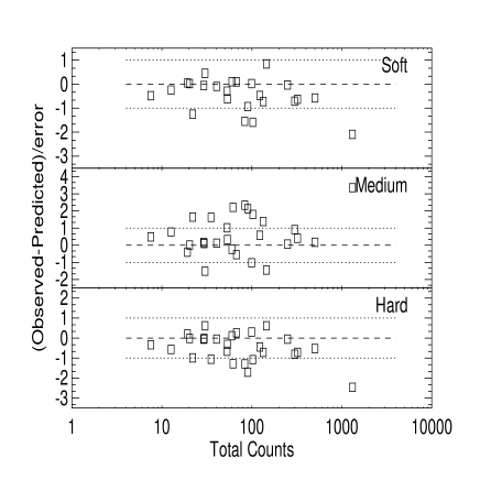
Figure 10: The predicted minus observed counts for the clusters. The dotted lines denote $1\sigma$ around zero.

As the use of a single temperature Raymond and Smith model reduced the residuals to the fit for the stars, we have attempted to fit a similar model to the three-colour data for the clusters. However, unlike the stars we find that in some cases a single temperature model does not reduce the residuals. This was particularly true of 240-564, the brightest source in our sample, where a single temperature fit to the three-colour data gave a high ($>10$ keV) temperature. Based on the residuals to a power-law fit, 240-564 would be expected to have a relatively low temperature. For this object we have been able to extract a high resolution spectrum which we have fitted using XSPEC. Figure 11 shows the fits both to the central region of the cluster and to an annular region surrounding the centre. As expected from the residuals, the temperature is low. There is also an apparent reduction in temperature towards the centre, implying that this cluster at least has a cooling flow. It is therefore clear that since three-colour data gave a high temperature we cannot use the temperatures derived for the clusters with any degree of certainty. We have extended the method to four or five colours on a number of the clusters within the RIXOS sample and this work shows that, with the extra channels, the method gives results that are consistent with higher resolution data. Such an extension to more colours is beyond the scope of this paper, however.

Figure 11: Colour plot of the Raymond and Smith fit to 240-564 in two regions, one in the inner most arc-minute, the other from an annular region surrounding the central core. There is a clear cooling of the temperature between the inner regions and the outer regions.

6.3 The Narrow Emission Line Objects

A subject of great interest is the X-ray emission from narrow emission line galaxies. Studies of the $\log N-\log S$ in fainter surveys such as the UK Deep survey show that the fraction of quasars at very faint flux levels declines, but that of NELGs rapidly increases (McHardy et al. 1998). Extrapolations to zero flux indicate that up to 50% of the X-ray background may be due to NELGs. The spectral shape of NELGs is therefore of crucial importance if we are to understand the nature of the soft X-ray background. However, a fundamental problem with this class of object is that the term NELG is a nebulous categorisation. They include hidden AGN, such as Seyfert 2’s where the emission is likely to be non-thermal and absorbed, to starburst galaxies and HII region galaxies, where the emission is thought to be thermal in nature and arising from shocked gas with a typical temperature of $0.5-1$ keV. From our work on stars, we know that we can distinguish between thermal and non-thermal sources on the basis of the fits to the three-colour data, so we should be able to estimate the fraction of thermal to non-thermal sources in the RIXOS sample.

There are 18 NELGs in RIXOS identified on the basis of their optical spectra. Figure 12 shows the distribution of observed minus predicted counts for the NELGs. In general, the NELGs seem consistent with a power-law, with only one source (122-16) showing a significant deviation in all three bands. This may imply thermal emission from this object, though preliminary studies of higher resolution data from 122-16 indicates that the X-ray spectrum is complex. Figure 14 shows the estimated mean slope and dispersion of the NELGs in comparison with the AGN and figure 13 shows the power-law slope as a function of redshift. This demonstrates no clear evidence for spectral evolution with redshift. Figure 13 does show that there is a large range of potential slopes, with some of the sources being very hard. At least one of these hard sources has been identified with a Seyfert 2 galaxy, which is entirely consistent with the flat spectral slope.

Thus the X-ray spectra of NELGs in the RIXOS sample are indistinguishable from those of the AGN. This is consistent with the fact that high resolution optical data on X-ray selected NELGs has shown that many objects classified as NELGs on the basis of low signal-to-noise data have broad components to the permitted lines (e.g. Boyle et al. 1995), and at least two H II region like galaxies have been observed to show strong X-ray variability more consistent with that seen in AGN (Boller et al. 1994, Bade et al. 1996). Further, HRI images of low-luminosity AGN show that the X-ray emission is mostly nuclear, again supporting the idea that the origin of the X-ray emission is nuclear in nature (Koratkar et al. 1995). Thus many objects classified as NELGs above the RIXOS flux limit may contain active nuclei.

However, it is important to note that the average slope that we find for the RIXOS NELGs is inconsistent with the average slope of a sample of much fainter NELGs from the UK Deep Field (Romero-Colmenero et al. 1996). In the latter study the average slope was $\alpha=0.45\pm 0.09$, a value that is more consistent with the average slope of the RIXOS clusters. There is clearly a discrepancy between the average properties of NELGs in the RIXOS sample and those found at much fainter fluxes which may imply some difference in the type of objects seen at the faintest fluxes. Another possibility is that there are more absorbed sources in the fainter samples which would pull down the average slope. Without higher resolution data and good signal to noise it is impossible to distinguish between these two possibilities.

Figure 12: The predicted minus observed counts for the NELGs ($\diamond$) and isolated galaxies ($\bigtriangleup$). The dotted lines denote $1\sigma$ around zero.

Figure 13: The fitted power-law slope versus the redshift for the NELGs in the RIXOS sample. No evolution of the power-law slope can be seen.

6.4 The AGN

By far the largest fraction of objects in the RIXOS sample have been classified as AGN. Unlike the stars and clusters of galaxies, a non-thermal model such as a power-law is likely to be an acceptable fit to the data, though in detail more complex models may be appropriate (e.g. Nandra and Pounds 1994). Figure 14 shows the mean slope and dispersion for the RIXOS AGN; we find $\alpha=1.05\pm 0.05$ and an intrinsic scatter of $0.55\pm 0.05$. These numbers are slightly steeper than those found for the EMSS AGN ($0.9\pm 0.05$ with a dispersion of $0.35\pm 0.04$), which sampled a harder energy range ($0.3-4$ keV) than the PSPC. However, this is much flatter than the slopes found for bright, nearby Seyferts observed with ROSAT (e.g. Walter and Fink 1993, Laor et al. 1994, Fiore et al. 1994) and is also flatter than the average slope found for the fainter AGN contained in the CCRS ($\alpha=1.3\pm 0.1$ Ciliegi et al. 1996). A slope of $\alpha=1$ is, however, consistent with what is believed to be the underlying power-law slope in nearby Seyferts (e.g. Nandra and Pounds 1994).

Figure 14: The values of the slope and dispersion for the RIXOS AGN (solid line) and the NELGs (dashed line). It is clear that the two samples are indistinguishable.

6.4.1 Goodness of fit for a power-law

Figure 15: The Predicted minus observed counts for the AGN. The dotted lines denote 1 sigma around zero.

Figure 15 shows the predicted minus observed total counts expressed in terms of the standard deviation for each spectral band for all the AGN. It is clear that for the majority of AGN a power-law fit is a reasonable representation of the spectral shape, as most of the data points lie within one sigma of the model. However, there do seem to be a number of AGN where the observed counts are significantly under estimated in the medium band. It is not clear what causes this deviation, as these sources seem to contain a mixture of slopes ranging from soft to hard. One possibility is that some contain a significant O VII edge, implying the presence of a warm absorber. However, three-colour data are not sufficient to determine the origin of this deviation and higher resolution data are required. We have extracted high resolution data for the source with the largest discrepancy in the soft band, source 258-001, which is sufficiently bright to warrant this. Analysis of these data shows evidence for an edge at 1.1 keV which has been tentatively identified with silicon (Mittaz et al. 1998). The ability to detect such a source shows the power of fitting three-colours to reveal peculiar features. From Figure 15 approximately 20% of sources appear to be deviant from a power-law model.

Without analysing all of the data at higher resolution, it is difficult to make strong claims about objects where a simple power-law does not appear to be an adequate description of the data. As noted in section 4, within the sample there are a number of sources which significantly deviate from the average spectrum. For example, some AGN have positive slopes, which correspond to those in the $C1<0$ region of the colour colour diagram. Such objects may be intrinsically absorbed and one (278-010) has sufficient counts to allow us to extract a higher resolution spectrum. On the assumption that the absorbing column is at the Stark et al. (1992) value of $1.94\times 10^{20}$ cm² a fit to these higher resolution data gives a slope of $\alpha=-1.17\pm 0.2$, consistent with the value fitted to the three-colour data. However, if we fit an intrinsic column in addition to the galactic $N_{H}$, we detect an instrinsic column at $>90$% confidence with a fitted power-law slope of $\alpha=(1.4^{+2.3}_{-1.7})$ and a best fit intrinsic $N_{H}$ of $(6^{+6}_{-4})\times 10^{21}$ cm^-2 (68% confidence limits). Figure 16 shows the 68%, 90% and 99% contours of the intrinsic absorption plotted against power-law slope. On the assumption that this hold true for the other AGN with $C1<0$ we can conclude that $\sim$5% of the RIXOS AGN sample show detectable amounts of intrinsic absorption. We note that trends between the fitted X-ray and optical spectral slopes, and between the X-ray spectral slope and the ratio of X-ray to optical flux, of RIXOS AGN have also be interpreted as being due to the effects of absorption (Puchnarewicz et al. 1996).

From the fitted power-law slopes it is moreover clear that there are not only hard sources, but also those which have slopes significantly steeper than $\alpha=1$. We have taken the object with the steepest slope which has a sufficiently large number of counts (227-301) and have extracted higher resolution X-ray data for it. A single power-law gives a very bad fit, with a $\chi^{2}_{\nu}$ of 6.8. We therefore fitted the data with a power-law and black-body model (to represent any soft excess), and the fit improved dramatically, with a $\chi^{2}_{\nu}$ of 0.56. The best fit parameters give a power-law slope of $\alpha=0.7\pm 0.7$ (68%) and a black-body temperature of $0.0085\pm 0.001$ keV (68%) (Figure 17). The value of the power-law slope is now consistent with the average for the RIXOS AGN, and the black-body component has a similar temperature to that seen the USS sample (Thompson and Cordova 1994). It is therefore clear that RIXOS contains a range of objects, from intrinsically absorbed AGN and those with strong soft excesses to objects with absorption edges. The high resolution data show that fits to the three-colour data can give sufficient information to separate out those objects which have non-standard X-ray spectra.

Figure 16: The contour plot of power-law slope against $N_{H}$ for 278-010. Intrinsic absorption can be clearly seen

Figure 17: A multicomponent fit to the X-ray spectrum of 227-301. The best fit model (black body and power-law) is shown

6.4.2 Spectral Evolution

A further question of interest is whether there is any evolution of the X-ray spectral slope of AGN with redshift. The nature of any such spectral evolution has consequences for both our understanding of the X-ray emitting process and the nature of the X-ray background. Figure 18 shows the distribution of slopes as a function of redshift, where we have used variously sized redshift bins. It is apparent from Figure 18 that there is no evidence for any spectral evolution at all. This lack of evolution in the spectral slopes is consistent with the results of other similar samples (e.g. Ciliegi et al. 1996). To investigate this further, we have recalculated the intrinsic slope and dispersion for AGN below and above a redshift of 1, where we have approximately equal numbers of AGN in each of the two bins. From figure 19 it is clear that the slopes and dispersions are effectively identical for objects above and below the redshift divide. As noted by Ciliegi et al. (1996), the fact that there is no apparent spectral evolution implies that the power-law spectrum in the AGN rest frame extends from soft X-rays out to at least 8 keV with the same slope. This excludes models with strong or hot soft excesses as being typical of AGN in the RIXOS sample.

Figure 18: Fitted slopes for the RIXOS AGN as a function of redshift. Each panel shows the data binned into successively bigger redshift bins with the error bar representing the RMS scatter about the mean, and shows that there is no evolution in the spectral slope. In the case of the middle two panels, the last two data points contain a single object and the plotted error is simply the error on the fit to those objects.

Figure 19: Intrinsic slope and dispersion for the RIXOS AGN separated into objects above and below a redshift of 1. It is clear that the two samples are identical implying no strong evolution in the spectral parameters of the AGN.

6.4.3 Interpretation and comparison with other surveys

The standard model for the X-ray emission from AGN derived from missions previous to GINGA and ROSAT was one of a medium energy power-law with a slope of $\alpha=0.7$ with many objects showing evidence for a soft X-ray excess. Such an excess is normally assumed to be due to the high energy tail of an accretion disk spectrum (e.g. Turner and Pounds 1988). However, with the advent of ROSAT and more recently ASCA, the situation has been found to be more complex. In detail it is often necessary to use models including reflection and warm absorbers as well as simple power-laws (e.g. Nandra and Pounds 1994). Approximately 50% of nearby Seyferts studied by Ginga have shown some evidence for warm absorbers, and evidence for an absorption line at 0.7 keV identified as O VII has even been found in PSPC data alone (e.g. Nandra and Pounds 1992).

Over the past decade there has been a lot of work on soft X-ray surveys of AGN and a number of samples have been compiled. The largest of these is the EMSS (Gioia et al. 1991) which consists of 421 AGN detected in the $0.5-4.5$ keV band. Maccacaro et al. (1988) found a mean spectral index for the AGN of $\alpha=1.03\pm 0.05$ with a dispersion of $\sigma=0.36$. Later surveys indicated that there may be an average steepening of the spectrum towards softer energies. The Ultra-Soft Survey from Einstein showed that AGN selected below 0.5 keV have an average slope of $\alpha=1.45$ (Thompson and Cordova 1994). The EXOSAT High Galactic Survey (HGLS), which covered the energy range 0.2 - 2 keV, was consistent with a mean spectral slope of $\alpha=1.3$ (Giommi et al. 1988) and work on ROSAT PSPC observations have indicated that the average spectrum of nearby bright AGN is about $\alpha=1.5$ (e.g. Walter and Fink 1993). Recently Schartel et al. (1996) used the ROSAT all-sky survey data for the QSOs in the Large Bright QSO survey and found a mean energy index of $\alpha=1.70\pm 0.2$ for the radio-quiet QSOs. Moving to higher redshift samples, Bechtold et al. (1994) found $\alpha=1.15\pm 0.14$ for a sample of high redshift, radio-quiet quasars and Reimers et al. (1995) found $\alpha=1.25\pm 0.2$ for another high redshift sample. It is difficult to make general statements on the basis of these different samples, however, since each has its own selection criteria and may therefore sample different populations of sources.

None of the above samples is directly comparable to RIXOS, either because of they are optically selected, or select bright X-ray sources, both of which can favour AGN with soft X-ray spectra (Puchnarewicz et al. 1996). There are, however, ROSAT serendipitous surveys with which a direct comparison should be more meaningful, although none are as large and/or complete as RIXOS. The CCRS, which has a similar flux limit to RIXOS, has a reported average slope which lies between the EMSS average and the average for the brighter samples, with $\alpha=1.3\pm 0.1$ (Ciliegi et al. 1996). At the very faintest fluxes, the average spectral slopes for QSOs in the UK Deep survey is $\alpha=0.96\pm 0.03$ (Romero-Colmenero et al. 1996) which is consistent with the EMSS. The spectrum of the QSOs in another deep survey has an average of $\alpha=1.23\pm 0.04$ (Almaini et al., 1996). Both the Ciliegi and the Almaini samples are therefore softer than the RIXOS average of $\alpha=1.05\pm 0.05$.

The largest difference is between the CCRS sample and RIXOS. Although the discrepancy is only at the two sigma level, it would be expected that these two samples would give essentially identical results, as the flux limits for the CCRS are only slightly lower than for RIXOS. However, the analysis techniques are different. From the simulations described in Section 5.3 it would be expected that the hardness ratio method used in the CCRS would give an average slope that was slightly softer than the ‘true’ value. We have attempted to re-analyse the CCRS data using the method used for the RIXOS sample. However, because accurate positions are not quoted for sources in the CCRS, it has not been possible to analyse the CCRS in exactly the same way as for RIXOS since we cannot unambiguously identify all the X-ray sources. Nevertheless Figure 20 shows the comparison between the RIXOS sample and our best estimate for the CCRS sample analysed using the Cash method, and the discrepancy between the two is reduced. The revised average slope of the CCRS, $1.16\pm 0.1$, is now consistent with the RIXOS sample at $1\sigma$ implying that the apparent difference between the two samples was caused at least in part by the bias introduced by using hardness ratios. The difference between the two dispersion estimates is likely to be caused by the assumption of a gaussian distribution of slopes rather than necessarily representing a real difference between the two samples.

Figure 20: A comparison of the RIXOS average slope and dispersion for the AGN (solid contour) and the estimated spectral slope and dispersion for the CCRS (dashed contour). Both contours have been obtained in precisely the same way, using the Cash statistic

From the range of different slopes obtained from different samples it is clear that the spectral distribution of AGN is quite complex and that source selection effects can play a dominant role in determining the average slope within a given sample. Nevertheless, the evidence increasingly suggests that faint X-ray selected AGN such as those found in ROSAT serendipitous surveys have a mean slope close to $\alpha=1$. Such an index is close to the value estimated to be the underlying intrinsic X-ray spectrum in Seyferts when effects such as reflection and a warm absorber are taken into account (Nandra and Pounds 1994). It is also close to the value of the inferred spectral slope seen in the IR, giving rise to claims that there is a power-law of energy index 1 underlying the observed spectrum from the IR to the X-ray range (e.g. Elvis et al. 1986). Deviations from this average slope can then be caused by additional processes such as soft X-ray excesses, warm absorbers and reflection, the effects of which are likely to be a function of redshift and/or luminosity. Some of these additional effects have already been observed in some high redshift objects. For example warm absorbers have been detected so far in two quasars, 3C351 (Fiore et al. 1993) and MR2251-178 (Pan, Stewart and Pounds 1990) though it is unclear how prevalent they are. However, without a detailed study of objects contained within RIXOS and other similar samples it is not possible to determine the proportion of objects in which these extra effects are important.

One final question needs to be addressed, and that is the effect of intrinsic absorption. Observations of selected high redshift quasars have indicated that absorption may be important in some objects (Elvis et al. 1994). High resolution spectra of CCRS AGN with sufficient counts to determine $N_{H}$ show only one object out of 36 AGN with evidence for significant absorption (Ciliegi et al. 1996), while in the data of Almaini et al. (1996) two out of nine objects require extra absorption. Selection effects may be at work here, since a source that is absorbed will appear fainter than the same source that is not, and the constraints on spectral fits are obviously better for brighter sources. However, from the X-ray colour-colour data there are indications that at least $\sim$ 5% of the RIXOS AGN have detectable absorption based on the X-ray data alone. This fraction is fairly secure because even at the flux cut-off of $3\times 10^{-14}$ ergs cm^-2 s^-1 RIXOS sources contain significant numbers counts. This is confirmed by simulations. We have constructed 1000 datasets with the same flux distribution and assumed slope distribution ($\alpha=1$ and $\sigma=0.55$) as the RIXOS sample and have analysed these datasets in exactly the same way as discussed in section 4. Out of the 1000 simulated datasets, only one of the simulated datasets have as many AGN in the $C1<0$ region of the colour-colour plot as are actually seen, as illustrated in Figure 21.

Figure 21: A histogram showing the number of times a given number of hard ($C1<0$) sources were found in simulated samples of RIXOS AGN. The simulated samples have the same flux and spectral distribution as the RIXOS AGN with a mean $\alpha=1$ and dispersion $\sigma=0.55$. Only one of the simulated datasets have as many hard sources as were seen the the RIXOS sample of AGN.

Even in those samples with much lower flux limits than exist in the RIXOS samples there is no evidence for extra absorption being required for the majority of the QSO part of the sample. Therefore, based on the X-ray data alone, there is no strong evidence for absorption playing a major role in the X-ray spectra of faint AGN and such effects only exist at the $\sim 10$% level.

7 Analysis of the whole RIXOS sample

Figure 22: Fits to the whole RIXOS dataset, consisting of 1762 objects. The top panel shows the power-law slope fit to all the data assuming galactic $N_{H}$. The second panel shows the data averaged in 6 flux bins, together with the standard error. A clear trend can be seen, with the average hardening with lower fluxes. The third panel shows the standard deviation of the data around the mean. The bottom panel shows the fitted average slope and error in each flux bin. This method essentially biases against extreme outliers, and is more representative of the mode of the distribution. These data show no strong correlation with flux. In all cases the dashed line is representative of the mode of the slopes.

Finally, we have analysed the whole RIXOS sample, including all sources in all RIXOS fields down to the detection limit of each field, containing 1762 sources. Even though we do not have identifications for most of the sources with a flux below $3\times 10^{-14}$ ergs cm^-2 s^-1 we can still study the spectral shape of the faintest sources which are precisely those which will contribute most to the soft X-ray background. Recent work has indicated that there may be a correlation between the average spectral slope and flux (Hasinger et al. 1993, Vikhlinin et al. 1995). Vikhlinin et al. (1995) analysed 130 ROSAT fields and extracted average spectra over a range of flux bins. They showed a correlation between source flux and spectral index, with bright sources ($>2\times 10^{-13}$ ergs cm^-2 s^-1) having average slopes close to 1.3, and faint sources ($<10^{-14}$ ergs cm^-2 s^-1) having average slopes close to 0.5. As noted by Vikhlinin et al., the average slope of 0.5 is close to that obtained for the soft X-ray background.

The exact significance of this correlation is, however, unclear since Vikhlinin et al. used either hardness ratios, which in the case of the faintest sources will have a bias to softer slopes (see section 5.3), or summed up all the sources in a flux bin and fitted multi-channel data with models using $\chi^{2}$. While summing up the data will allow higher signal-to-noise at a higher resolution, it can only give information on the average properties of the sources and not on the distribution of slopes in a given flux band.

By using the Cash statistic technique on three-colour data we can avoid problems of biases. We have analysed the whole RIXOS sample containing 1762 sources including sources which extend down to a flux of $4\times 10^{-15}$ ergs cm^-2 s^-1. Figure 22 shows the fits to the whole sample as a function of flux both as a scatter plot and binned into flux bins. The second panel shows the average of the slopes in each flux bin which is the equivalent of the Vikhlinin et al. data. As with the sample of Vihklinin et al. there is a clear trend towards harder spectra at lower flux limits in the latter. Above the RIXOS flux limit there is no significant hardening, while there is a significant deviation below $\sim 2\times 10^{14}$ ergs cm^-2 s^-1. However, unlike the Vihklinin sample we can look at the distribution of slopes within a flux bin. The top panel of Figure 22 makes it clear that the majority of sources do not show a trend to harder slopes at lower flux limits. To highlight this further, we have fitted the mean slope and dispersion within each flux bin in the same way we have done for the RIXOS sample (section 6). The bottom panel shows the fitted average slope as a function of flux and it is clear that there is no significant trend. The most obvious explanation for this discrepancy between the arithmetically averaged data and the fitted average value is that there are changes in the distribution of slopes within a flux bin rather than a global change in the spectral slope. This is supported by the third panel which shows an increase in the measured standard deviation of the data with decreasing flux. In the RIXOS data it is clear that there are a number of very hard sources below a flux of $3\times 10^{-14}$ ergs cm^-2 s^-1. These sources would bias the mean but, as outliers, they would not have a significant effect on fits of a gaussian distribution to the slopes, exactly as observed. If we look at those sources where $\alpha<0$, then 20% of sources below $3\times 10^{-14}$ ergs cm^-2 s^-1 satisfy this condition. However, if we look at all those sources with fluxes greater than $3\times 10^{-14}$ ergs cm^-2 s^-1, then only 13% of the sources satisfy this criterion. It is therefore clear that as we go to fainter fluxes a higher proportion of the sources are very hard. From studies of deep ROSAT pointings it is unlikely that there are a significant number of stars at faint fluxes, and it is more likely that the sources with hard spectra are an absorbed population. One obvious candidate for these sources are Seyfert 2 galaxies. Such sources are both hard and faint relative to un-obscured AGN and would therefore give the observed distribution which has more hard sources at fainter fluxes.

7.1 The nature of the soft X-ray background

One question that has been highlighted by recent ROSAT observations is the nature of the soft X-ray background. It has been known for many years that the average slope of the soft X-ray background is $\alpha=0.4$ (for a review see Fabian and Barcons 1992). This spectrum is inconsistent with the average spectrum of (relatively bright) AGN. From the deepest surveys undertaken to date it is clear that a significant fraction of the X-ray background is made up of emission from narrow emission line galaxies (NELGs), an amorphous classification that may include Seyfert 2 galaxies as well as starburst galaxies and LINERS. However, the average spectrum of the RIXOS NELGs is also too soft to explain the soft X-ray background.

In contrast, the mean spectrum of NELGs at fainter flux levels is consistent with the X-ray background (Romero-Colmenero et al. 1996) and harder than that of AGN even in the same flux range. In the previous section, we showed that the hard overall mean spectrum at faint fluxes is caused by a population of very hard sources (i.e. harder than the background). These bias the mean source spectral slope to a value which is consistent with the slope of the background.

A combination of two possible explanations may account for the slope of the X-ray background, given that the NELGs are likely to be a mixture of intrinsic source types. There may be a genuine change in the dominant emission mechanism between the bright RIXOS NELGs and those identified in deep surveys, with the emission from faint NELGs being dominated by a hot continuum source (for example hot gas, perhaps associated with an extended halo rather than the galactic nucleus); or the very hard sources which we identify in the extended RIXOS sample may be an absorbed population consisting, say, of Seyfert 2 galaxies (cf. Grindlay and Luke 1990). More sensitive individual X-ray spectral observations of a sample of faint sources will be needed to resolve this question.

8 Conclusions

RIXOS is a flux limited, nearly complete sample of X-ray selected sources. We have demonstrated that for such a sample it is possible to obtain useful spectral information even down to very faint limits, as long as the correct statistic is used. In contrast, a simple hardness ratio method, which has been used by a number of authors to determine the spectral slope for faint sources, is shown to bias in the inferred power-law slope towards a steeper spectrum. The use of three-colour data allows some discrimination between thermal and non-thermal X-ray emission, at least for relatively bright sources. We have determined the spectral characteristics for each sub-category of sources within the RIXOS survey:

• Though little can be said directly about the X-ray spectra of the stars, the use of three-colour data demonstrates the ability of the method to discriminate between thermal and non-thermal sources.

• Most of the RIXOS clusters are consistent with the majority of the emission arising from hot ($>3$ keV) gas. There are some clusters where there is evidence for a lower temperature, which may indicate the presence of a cooling flow.

• On average, the NELGs have X-ray spectra that are consistent with the spectra of the AGN and may indicate that many of the NELGs found in RIXOS are, in fact, low-luminosity AGN. This is at variance with the X-ray spectra of NELGs found from deep X-ray surveys, where the average slope is much harder. The NELGs observed in deep X-ray surveys are then either a more absorbed population of sources, or the X-ray emission in the faintest NELGs arises from some other mechanism other than an AGN non-thermal power-law.

• The AGN have an average slope of $\alpha=1.05\pm 0.05$ with no evidence for spectral evolution. This average slope is somewhat harder than the averages found for other samples of soft X-ray selected AGN. However, the inappropriate use of hardness ratios will have softened the average slopes in other samples. The value of $\alpha=1.05$ is consistent with the naked power-law expected from AGN, implying that the X-ray spectrum of the RIXOS AGN is relatively uncontaminated by processes such as reflection and absorption. Since many of the previous X-ray selected samples concentrated on low redshift/low luminosity AGN, part of the discrepancy between RIXOS and other samples may be ascribed to the effect of redshift and/or luminosity on the processes that modify the underlying power-law.

• Analysis of the whole RIXOS sample confirms the presence of a flux dependent spectral slope (Hasinger et all 1993, Vikhlinin et al. 1995). However, we have been able to investigate the cause of this correlation and the most likely explanation is of an increasing proportion of very hard sources rather than an average hardening of the spectra.

Landscape table to go here.

Landscape table to go here.

Landscape table to go here.

Landscape table to go here.

Landscape table to go here.

Landscape table to go here.

Landscape table to go here.

Landscape table to go here.

Landscape table to go here.

Landscape table to go here.

Landscape table to go here.

Landscape table to go here.

Landscape table to go here.

References

- [Almaini et al.1996] Almaini O., Shanks T., Boyle B.J., Griffiths R.E., Roche N., Stewart G.C., Georgantopoulos I., 1996, MNRAS, 282, 295
- [Bade et al.1996] Bade N., Komossa, S., Dahlem, M., 1996, A&A, 309, 35L
- [Bechtold et al.1994] Bechtold, J., Elvis, M., Fiore, F., Kuhn, O., Cutri, R.M., McDowell, J.C., Rieke, M., Siemiginowska, A., Wilkes, B.J., 1994, AJ, 108, 759
- [Boller et al.1994] Boller, T., Fink, H., Schaeidt, S., 1994, A&A, 291, 403
- [Bowyer et al.1994] Bowyer S., Lieu R., Lampton M., Lewis J., Wu X., Drake J.J., Malina R., 1994, ApJS, 93, 569
- [Boyle et al.1994] Boyle, B.J., Shanks, T., Georgantopoulos, I., Stuart, G.C., Griffiths, R.E., 1994, MNRAS, 271, 639
- [Boyle et al.1995] Boyle, B.J., McMahon, R.G., Wilkes, B.J, Elvis, M., 1995, MNRAS, 272, 462
- [Branduardi-Raymont et al.1995] Branduardi-Raymont G., Mason K.O., Warwick R.S., Carrera F.J., Graffagnino V.G., Mittaz J.P.D.,E Puchnarewicz E.M., Smith P.J., Barber C.R., Pounds K.A., Stewart G.C., McHardy I.M., Jones L.R., Merrifield M.R., Fabian A.C., McMahon R.G., Ward M.J., George I.M., Jones M.H., Lawrence A., Rowan-Robinson M., 1994, MNRAS, 270, 947
- [Carrera1998] Carrera F.J., 1998, MNRAS, submitted
- [Cash1979] Cash J., 1979, ApJ, 228, 939
- [Castander et al.1995] Castander F.J., Bower R.G., Ellis R.S., Aragon-Salamanca A., Mason K.O., Hasinger G., McMahon R.G., Carrera F.J., Mittaz J.P.D., Pérez–Fournon I., Lehto H,J., 1995, Nature, 377, 39
- [Ciliegi et al.1996] Ciliegi P., Elvis, M., Wilkes, B.J., Boyle, B.J., McMahon, R.G., 1996, MNRAS, 284, 401
- [Elvis et al.1986] Elvis, M., Green, R.F., Bechtold, J., Scmidt, M., Neugebauer, G., Soifer, B.T., Mathews, K., Fabbiano, G., 1986, ApJ, 310, 291
- [Hasinger et al.1993] Hasinger G, Burg R., Giacconi R., Hartner G., Schmidt M., Trumper J., Zamorani G., 1993, A&A, 275, 1
- [Fabian and Barcons1992] Fabian, A.C. and Barcons, X., 1992, ARA&A, 30, 429
- [Fiore et al.1993] Fiore, F., Elvis, M., Mathur, M., Wilkes, B.J., McDowell, J.C., 1993, 415, 129
- [Fiore et al.1994] Fiore, F., Elvis, M., McDowell, J.C., Siemiginowska, A., Wilkes, B.J., 1994, ApJ, 431, 515
- [Gioia et al.1990] Gioia I. M., Maccacaro T., Schild R. E., Wolter A., Stocke J. T., Morris S. L., Henry J. P., 1990, ApJS, 72, 567
- [Giommi et al.1991] Giommi P., Tagliaferri G., Beuermann K., Branduardi-Raymont G., Brissenden R., Graser U., Mason K. O., Mittaz J. P. D., Murdin P., Pooley G., Thomas H. -C., Tuohy I., 1991, ApJ, 378, 77
- [Grindlay and Luke 1990] Grindlay, J.E. and Luke, M., 1990, in: High resolution X-ray spectroscopy of cosmic plasmas, Cambridge University Press, 276
- [Koratkar et al. 1995] Koratkar A., Deustua S.E., Heckman T., Filippenko A.V., Ho L.C., Rao M., 1995, ApJ, 440, 132
- [Loar et al.1994] Laor, A., Fiore, F., Elvis, M., Wilkes, B.J., McDowell, J.C., 1994, ApJ, 435, 611
- [Loredo1990] Loredo T.J., 1990, in: Maximum Entropy and Bayesian Methods, Ed. P.F. Fougére, 81
- [Maccacaro et al.1988] Maccacaro T., Gioia I.M., Wolter A., Zamorani G., Stocke J.T., 1988, ApJ, 326, 680
- [Mason et al.1997] Mason K.O. et al., 1998, in preparation
- [McHardy et al.1998] McHardy I.M. et al., 1997, MNRAS, in press.
- [Mittaz et al.1997] Mittaz, J.P.D. et al., 1998, in preparation
- [Nandra & Pounds1992] Nandra, K. and Pounds, K.A., 1992, Nature, 359, 215
- [Nandra & Pounds1994] Nandra K. & Pounds, K.A., 1994, MNRAS, 268, 405
- [Pan, Stewart & Pounds1990] Pan, H.C., Stewart, G.C., Pounds, K.A., 1990, MNRAS, 242, 177
- [Page et al.1996] Page M.J., Carrera, F.J., Hasinger, G., Mason, K.O., McMahon, R., Mittaz, J.P.D., Barcons, X., Carballo, R., Gonzalez-Serrano, I., Pérez–Fournon, I., 1996, MNRAS, 281, 579
- [Pounds et al.1993] Pounds K.A. et al., 1993, MNRAS, 260, 77
- [Press et al.1992] Press W.H., Teukolsky S.A., Vetterling W.T., Flannery B.P., 1992, Numerical Recipes, Cambridge University Press, 617
- [Puchnarewicz et al.1996a] Puchnarewicz E.M., Mason K.O., Romero-Colmenero E., Carrera F.J., Hasinger G., McMahon R., Mittaz J.P.D., Page M.J., Carballo R., 1996, MNRAS, 281, 1243
- [Puchnarewicz et al.1996] Puchnarewicz, E. M., Mason, K. O., Carrera, F. J., Brandt, W. N., Cabrera-Guera, F., Carballo, R., Hasinger, G., McMahon, R. G., Mittaz, J. P. D., Page, M. J., Perez-Fournon, I., Schwope, A., 1997, MNRAS, 291, 177
- [Reimers et al.1995] Reimers, D., Bade, N., Schartel, N., Hagen, H.-J., Engels, D, Toussaint, F., 1995, A&A, 296, 49
- [Romero-Colmenero et al.1996] Romero-Colmenero E. Branduardi-Raymont, G., Carrera, F.J., Jones, L.R., Mason, K.O., McHardy, I.M., Mittaz, J.P.D., 1996, MNRAS, 282, 94
- [Romero-Colmenero et al.1997] Romero-Colmenero E. et al., 1997, in preparation
- [Sarazin1986] Sarazin C.L., 1986, Reviews of Modern Physics, 58, 1
- [Schmitt et al.1990] Schmitt J.H.M.M., Collura A., Sciortino S., Vaiana G.S., Harnden F.R., Rosner R., 1990, ApJ, 365, 704
- [Schartel et al.1996] Schartel, N., Walter, R., Fink, H,H., Trümper, J., 1996, A&A, 307, 33
- [Snowden et al.1994] Snowden S.L., McCammon D., Burrows D.N., Mendenhall J.A., 1994, ApJ, 424, 714
- [Thompson & Cordova1994] Thompson, R.J. and Cordova, F.A., 1994, ApJ, 434, 54
- [Turner & Pounds1988] Turner, T.J. and Pounds, K.A., 1988, MNRAS, 232, 463
- [Vihklinin et al.1995] Vikhlinin, A., Forman, W., Jones, C., Murray, S., 1995, ApJ, 451, 564
- [Walter & Fink1993] Walter, R. & Fink, H.H., 1993, A&A, 274,