Searching for the non-gaussian signature of the CMB secondary anisotropies

Abstract

In a first paper (Forni & Aghanim 1999), we developed several statistical discriminators to test the non-gaussian nature of a signal. These tests are based on the study of the coefficients in a wavelet decomposition basis. In this paper, we apply them in a cosmological context, to the study of the nature of the Cosmic Microwave Background (CMB) anisotropies. The latter represent the superposition of primary anisotropy imprints of the initial density perturbations and secondary ones due to photon interactions after recombination. In an inflationary scenario (standard Cold Dark Matter) with gaussian distributed fluctuations, we study the statistical signature of the secondary effects. More specifically, we investigate the dominant effects arising from the Compton scattering of CMB photons in ionised regions of the Universe: the Sunyaev-Zel’dovich effect of galaxy clusters and the effects of a spatially inhomogeneous re-ionisation of the Universe.

Our study specifies and predicts the non-gaussian signature of the secondary anisotropies induced by these scattering effects. We find that our statistical discriminators allow us to distinguish and highlight the non-gaussian signature of a process even if it is combined with a larger gaussian one. We investigate the detectability of the secondary anisotropy non-gaussian signature in the context of the future CMB satellites (MAP and Planck Surveyor).

1 Introduction

The Cosmic Microwave Background (CMB) is a powerful tool for cosmology. As the CMB temperature anisotropies represent the superposition of primary (before matter-radiation decoupling) and secondary (after decoupling) fluctuations, the study of the anisotropies gives a direct insight into both the early Universe (and initial conditions) and the formation and evolution of cosmic structures. One of the goals of cosmology is to characterise the initial density perturbations which gave rise to those structures: galaxies and galaxy clusters. The statistical properties of the initial perturbations provide part of the necessary information for this characterisation. They can indeed be used to test and constrain the cosmological models and scenarios of structure formation. The angular power spectrum of the temperature fluctuations is one of the most important statistical quantities for CMB anisotropy studies. In fact, it allows the evaluation of the main cosmological parameters ($\Omega_{b}$, $\Omega_{0}$, $\Lambda$, $n$, …) defining our Universe (Jungman et al. 1996). Some of the first constraints on the cosmological parameters came from CMB anisotropy measurements made by the COBE satellite (Smoot et al. 1992; Wright et al. 1992). The statistical properties of the CMB anisotropies give us information, in particular, on the physical process at the origin of the initial density fluctuations. Two classes of scenario account for the initial seeds of the structures. One is the “inflationary model” (Guth 1981; Linde 1982) in which the density perturbations result from the quantum fluctuations of scalar fields in the very early Universe. The other invokes the topological defects which themselves correspond to symmetry breaking in the unified theory (cosmic string, textures) (Vilenkin 1985; Bouchet 1988; Stebbins 1988; Turok 1989; Pen et al. 1994). Several studies have shown that the two scenarios predict different angular power spectra (Coulson et al. 1994; Albrecht et al. 1996; Magueijo et al. 1996). These differences of amplitude and/or shape represent rather tight constraints on the models. The statistical nature of the primary density perturbations, and hence their origin, is also encompassed within the distribution of the CMB anisotropies. The brightness, or temperature, distribution is indeed directly induced by the primeval mass or density distribution. If the initial perturbations result from an inflationary process the primary anisotropy distribution is gaussian. If the perturbations are generated by topological defects the anisotropy distribution is non-gaussian. The latter predict very specific patterns distinguishable from a gaussian random field. It is thus necessary to find statistical methods to test non-gaussianity and to separate primary and secondary non-gaussianity.

Several studies have been performed to test the CMB gaussianity. Traditional methods use the brightness or temperature distribution and their n$th$ order moments or their cumulants (Ferreira et al. 1997). Other methods are based on the n-point correlation functions or their spherical harmonic transforms (Luo & Schramm 1993; Magueijo 1995; Kogut et al. 1996; Ferreira & Magueijo 1997; Ferreira et al. 1998; Heavens 1998; Spergel & Goldberg 1998). Non-gaussianity can also be tested through topological discriminators based on pattern statistics (Coles 1988; Gott et al. 1990). Alternative methods test the non-gaussianity in the Fourier or wavelet space (Ferreira & Magueijo 1997; Hobson et al. 1998; Forni & Aghanim 1999).

In addition to the intrinsic statistical properties of the CMB anisotropies, the secondary fluctuations associated with cosmic structures (e.g., galaxies and galaxy clusters) induce non-gaussian signatures which could originate from point-like sources, peaked profiles, or from geometrical characteristics such as sharp edges or specific patterns. Future high sensitivity and high resolution CMB observations (e.g., MAP and Planck Surveyor satellites) will provide data sets which should allow detailed tests of the primary anisotropy distribution. A detailed study of the non-gaussianity associated with secondary sources could be used to discriminate between the inflationary and topological defect models.

The present study deals with this first step: to predict and to specify the non-gaussian signature of the secondary anisotropies arising from the scattering of CMB photons by the ionised matter in the Universe. We apply the statistical discriminators developed in Forni & Aghanim (1999) to combinations of gaussian primary and secondary non-gaussian anisotropies. We take into account the contribution of a population of galaxy clusters through the Sunyaev-Zel’dovich (SZ) effect (Sunyaev & Zel’dovich 1980) as well as the effect of a spatially inhomogeneous re-ionisation of the Universe (Aghanim et al. 1996; Gruzinov & Hu 1998; Knox et al. 1998). The non-gaussian signature due to secondary anisotropies associated with weak gravitational lensing have been investigated in previous studies (Seljak 1996b; Bernardeau 1998; Winitzki 1998).

In section 2, we present the astrophysical contributions we take into account in our study. We then briefly present the statistical tests and detection strategy in section 3. We apply our tests to the combinations of primary and secondary anisotropies due to inhomogeneous re-ionisation alone in section 4, and to a configuration including the SZ effect of galaxy clusters in section 5. In section 6, we investigate the detectability of the non-gaussian signature for a MAP-like and a Planck-like instrumental configuration. Finally, in section 7, we discuss our results and present our conclusions.

2 Astrophysical contributions

The temperature anisotropies of the CMB contain the contributions of both the primary cosmological signal, directly related to the initial density fluctuations, and the foreground contributions amongst which are the secondary anisotropies. The secondary anisotropies are generated after matter-radiation decoupling. They arise from the interaction of the CMB photons with the matter and can be of a gravitational type (e.g. Rees-Sciama effect (Rees & Sciama 1968)), or of a scattering type when the matter is ionised (e.g. SZ or Ostriker-Vishniac effect (Ostriker & Vishniac 1986; Vishniac 1987)). In our study we adopt a canonical inflationary standard CDM (Cold Dark Matter) model for the generation of the primary anisotropies.

We simulate maps of the three astrophysical processes of interest in our study: the primary and secondary fluctuations due to inhomogeneous re-ionisation and the SZ effect. For each process, we made 100 realisations of $512\times 512$ pixels (1.5 arcminute pixel size). This fairly large number of realisations allows us to have statistically significant results. They represent about 40% of the whole sky, equivalent to the “clean” fraction of the sky coverage available for CMB analysis. Indeed, we do not expect to be able to analyse regions of the sky that are highly contaminated by galactic emissions (dust, synchrotron and free free). These contaminated regions account, more or less, for the Galactic latitudes with $|b|<30^{\circ}$ ($\sim 60$% of the sky).

2.1 Primary CMB anisotropies

For the purpose of this study, that is the characterisation of the non-gaussianity from secondary anisotropies, we assume gaussian distributed primary fluctuations generated in an inflationary scenario. We choose the canonical standard CDM model, normalised to COBE data. The maps were generated using a code, kindly provided by P.G. Ferreira that generates square gaussian realisations given a power spectrum. The CMB power spectrum, displayed in figure 1, was computed using the CMBFAST code (Seljak & Zaldarriaga 1996).

2.2 Secondary CMB anisotropies

2.2.1 From inhomogeneous re-ionisation

The first generation of emitting objects ionises the surrounding gas of the globally neutral Universe at high redshifts. The resulting spatially inhomogeneous re-ionisation generates secondary anisotropies associated with the peculiar motion along the line of sight of ionised bubbles. This produces anisotropies with maximum amplitude at the degree scale, and with $(\delta T/T)_{rms}\sim 6.\,10^{-6}$. The anisotropies are about ten times smaller than the primary fluctuations and spectrally indistinguishable from them. We use the model of Aghanim et al. (1996), in which these objects are early ionising quasars with assumed lifetimes of $10^{7}$ yrs. The number of quasars is normalised to match the data at $z\sim 4$ and has been extrapolated for $4<z\leq 10$. The positions of the centres of the ionised regions are drawn at random in the $512\times 512$ pixel maps, and we assume a spherically symmetric gaussian profile for the temperature anisotropy. The size and amplitude of the anisotropies depend on the quasar luminosities and its light-on redshifts. We compute the skewness and kurtosis (third and fourth moments of the distribution) of the maps. All the maps exhibit a non-gaussian signature associated with an excess of kurtosis of the order of one, the skewness being null.

2.2.2 From Sunyaev-Zel’dovich effect

The Sunyaev-Zel’dovich effect represents the Compton scattering of the CMB photons by the free electrons of the ionised and hot intra-cluster gas. It results in the so-called thermal SZ effect which exhibits a peculiar spectral signature with a minimum at long wavelengths and a maximum at short wavelengths. When the cluster moves with respect to the CMB rest frame, the Doppler shift induces an additional effect called the kinetic SZ effect. It generates anisotropies with the same spectral signature as the primary ones. The temperature anisotropies generated by the clusters are thus composed of the thermal $(\delta T/T)_{th}$ and kinetic $(\delta T/T)_{ki}$ SZ anisotropies. We simulate both effects using an updated version (Aghanim et al. 1998) of the Aghanim et al (1997) model. The simulations use the $\beta$-model (Cavaliere & Fusco-Femiano 1978) to describe the gas distribution of each individual cluster. This description is generalised to a population of clusters derived from the Press-Schechter formalism (Press & Schechter 1974) and normalised to the X-ray temperature distribution (Viana & Liddle 1996). The positions of the cluster centres are drawn at random in the maps. Again we find a zero skewness but a strongly non-gaussian signature because the kurtosis is non-zero.

3 Statistical tests and detection strategy

In a previous study (Forni & Aghanim 1999), we developed statistical methods to search for non-gaussianity. The tests are based on the detection of gradients in the wavelet space. They use the statistical properties of a signal in wavelet space, namely the measurement of the excess of kurtosis (fourth moment, $\mu_{4}$, of a distribution) of the coefficients associated with the gradients. The predicted excess of kurtosis for a gaussian distribution is zero. If the non-gaussian signal is not skewed (third moment of the distribution is zero), any significant departure from gaussianity is indicated by a non-zero excess of kurtosis.

Figure 1: Scale windows corresponding to the 4 decomposition levels (in the spherical harmonics space) by the bi-orthogonal filter #3 (Villasenor et al. 1995). From right (scale I) to left (scale IV), the windows are centred around a multipole of $\sim 5600$,$\sim 2800$, $\sim 1400$ and $\sim 700$. Their respective Full Widths at Half Maximum are $(\Delta l)_{FWHM}\sim 4800$, $\sim 2400$, $\sim 1200$ and $\sim 600$. The solid line shows the normalised CMB primary anisotropy power spectrum.

The first test for non-gaussianity is based on what we call the multi-scale gradient. It is the quadratic sum of the wavelet coefficients associated with $(\partial/\partial x)^{2}+(\partial/\partial y)^{2}$ and we find it follows a Laplace distribution for a gaussian distributed signal. For sets of 100 statistical realisations wavelet filtered at four decomposition scales (Fig. 1), we compute the normalised excess of kurtosis with respect to the Laplace distribution ($k=\mu_{4}/\mu_{2}^{2}-6$) together with the standard deviations (with respect to the median excess of kurtosis).

The second statistical test uses the wavelet coefficients associated with the horizontal and vertical gradients ($\partial/\partial x$ and $\partial/\partial y$ derivatives). We also use the coefficients related to the diagonal gradients ($\partial^{2}/\partial x\partial y$ cross derivative), which are gaussian distributed for a gaussian signal. We then compute the normalised excess of kurtosis ($k=\mu_{4}/\mu_{2}^{2}-3$), with respect to a gaussian distribution and the standard deviations (with respect to the median) for all the realisations.

We apply the detection strategy proposed in Forni & Aghanim (1999) to demonstrate and to quantify the detectability of the non-gaussian signature. It is based on the comparison of a set of maps of the “real” observed sky to a set of gaussian realisations having the power spectrum of the “real sky”. The main advantage of this is that it can be reliably applied regardless of the power spectrum of the studied non-gaussian signal.

4 Analysis of the anisotropies: Primary + inhomogeneous re-ionisation

We first study the case of primary CMB anisotropies with secondary anisotropies due to inhomogeneous re-ionisation. The primary CMB anisotropies dominate at all scales larger than the cut off (at about 5 arcminutes). The non-gaussian signal is very small compared to the gaussian one. Indeed, the power spectrum of the secondary anisotropies represents, at most, less than 10% of the primary CMB power.

4.1 Multi-scale gradient

We compute the median value of the excess of kurtosis for the 100 realisations and the associated confidence intervals (Tab. 1). At the first decomposition scale the secondary anisotropies dominate the primary. We thus expect the non-gaussian signature of the secondary anisotropies to dominate, and indeed, we find a non-zero excess of kurtosis. At the two larger decomposition scales, the median value $k$ is marginally non-zero. The computed $\sigma$ values take into account the non symmetrical distribution of the kurtosis and exhibit a clear dichotomy between the upper ($\sigma_{+}$) and lower ($\sigma_{-}$) boundaries of the confidence interval. This suggests that non-gaussianity has been detected. If $k-\sigma_{-}$ for one realisation is larger than zero by a value of the order of, or larger than, $\sigma_{-}$; then this indicates a significant departure from gaussianity. If $k-\sigma_{-}$ is of the order of zero then, more sophisticated tests must be applied to conclude weather the “real sky” has a non-gaussian signature. At the second decomposition scale, the non-zero value of the median excess of kurtosis is possibly due to the sampling effects resulting from the sharp cut off in the primary CMB power spectrum at about 5 arcminutes (in a standard CDM model) combined with the rather narrow window filter we use in the analysis.

Scale	$k$	$\sigma_{+}$	$\sigma_{-}$
I	0.3	0.15	0.16
II	1.19	0.88	0.50
III	0.15	0.67	0.41

Table 1: The median excess of kurtosis $k$ of the multi-scale gradient coefficients, at four decomposition scales, computed over 100 realisations of the CMB primary + secondary anisotropies due to inhomogeneous re-ionisation. $\sigma_{+}$ $\sigma_{-}$ and define the confidence interval for one realisation.

4.2 Partial derivatives

Scale		$k_{1}$	$\sigma_{+}$	$\sigma_{-}$		$k_{2}$	$\sigma_{\pm}$
I	$\partial/\partial x$	0.04	0.02	0.02		-$10^{-4}$	0.02
II	&	0.12	0.06	0.05	$\partial^{2}/\partial x\partial y$	0.06	0.04
III	$\partial/\partial y$	0.02	0.09	0.07		0.02	0.08

Table 2: The median excess of kurtosis, at four decomposition scales, computed over 100 realisations of the sum of CMB and secondary anisotropies due to inhomogeneous re-ionisation. $k_{1}$ is given for the coefficients associated with the vertical and horizontal gradients, and $k_{2}$ is given for the cross derivative. The $\sigma$ values are the boundaries of the confidence interval for one statistical realisation.

The analysis of the coefficients, associated with the cross and the first derivatives (Tab. 2), exhibit non-zero median excess of kurtosis at the first two decomposition scales. At the third and fourth scales the obtained excess of kurtosis is very close to the values of the CMB primary anisotropies alone.

Figure 2: Excess of kurtosis computed over the wavelet coefficients of respectively $\partial/\partial x$ for the left panels, $\partial/\partial y$ for the centre panels and $\partial^{2}/\partial x\partial y$ for the right panels. The solid line is for CMB + non-gaussian secondary anisotropies due to patchy re-ionisation. The dashed line is for gaussian realisations, with the same power spectrum.

In order to illustrate the non-gaussian characteristics of the different statistical realisations, we plot (Fig. 2) the excess of kurtosis of the wavelet coefficients associated with the partial derivatives ($\partial/\partial x$ and $\partial/\partial y$) and the cross derivative $\partial^{2}/\partial x\partial y$. The solid line corresponds to the results obtained for the 100 realisations of a non-gaussian process made of the primary CMB + secondary anisotropies. Whereas the dotted line stands for the 100 gaussian test maps with same power spectrum as the studied process. The excesses of kurtosis are computed with the coefficients related to the horizontal gradient $\partial/\partial x$ (left panels), to the vertical gradient $\partial/\partial y$ (centre panels), and to the cross derivative $\partial^{2}/\partial x\partial y$ (right panels). For the gaussian signal, the excesses of kurtosis of the cross derivative coefficients are centred around zero whereas they are not for the first derivative coefficients. This indicates that the cross derivative coefficients better characterise gaussian signals. They thus seem more appropriate to test for non-gaussianity, even though the coefficients have smaller amplitudes. The results show a clear departure of the excess of kurtosis from zero at the two first decomposition scales, for the non-gaussian signal. At the third decomposition scale, the excess of kurtosis for the cross derivative becomes very weak, indicating a marginal detection of non-gaussianity.

Following the detection strategy of Forni & Aghanim (1999), we perform a set of 100 gaussian realisations with same power spectrum as the sum of CMB and inhomogeneous re-ionisation, and we compute the excess of kurtosis for both the multi-scale gradient and the partial derivative coefficients. The probability distribution function (PDF) of the excess of kurtosis, for the non-gaussian (solid line) and gaussian (dashed line) realisations, are plotted in figure 3.

Figure 3: Probability distribution functions, in percentage, of the excess of kurtosis computed with the multi-scale gradient coefficients (right panels) and with the cross derivative coefficients (left panels). The dashed line is for the gaussian test maps with same power spectrum as the non-gaussian signal (solid line). This signal is made of primary CMB anisotropies and secondary anisotropies due to inhomogeneous re-ionisation.

We display, in the left panels, the PDF for the cross derivative coefficients. In the right panels, we show the excess of kurtosis computed with the multi scale gradient coefficients. We note that investigating the statistical properties with the multi-scale gradient coefficients and cross derivative coefficients is quite complementary, because the multi scale gradient is related to $\partial/\partial x$ and $\partial/\partial y$. The detection of the non-gaussian signature is clear when the PDFs are clearly shifted. Our results show that the median excess of kurtosis of the multi scale gradient coefficients measures the non-gaussian nature of the secondary anisotropies due to inhomogeneous re-ionisation with a probability of 99.76% at the first decomposition scale. At all other scales, the detection level, for this discriminator, is below the one sigma limit. For the statistical test based on the cross derivative, the probability that the non-gaussianity is detected is 89.5% at the second decomposition scale. All the other scales show no significant departure from gaussianity.

5 Analysis of the anisotropies: including the SZ effect

Besides the secondary anisotropies that would arise in the context of an inhomogeneous re-ionisation of the Universe, there exist secondary anisotropies due to the SZ effect of galaxy clusters. In our study, we therefore add to the previous model the contribution of both thermal and kinetic SZ effects of a galaxy cluster population. We analyse the maps corresponding to the sum of CMB primary and secondary fluctuations (SZ + inhomogeneous re-ionisation) with a resolution of 1.5 arcminutes and the nominal Planck gaussian noise. The contribution of the thermal SZ effect, $(\delta T/T)_{th}$, is given at 2mm.

5.1 Multi-scale gradient

We compute the excess of kurtosis of the multi-scale gradient coefficients of the primary + secondary anisotropy maps. In Table 3, we note the extraordinarily large values of the median excesses of kurtosis $k$ with respect to the previously studied process (CMB primary anisotropies + secondary fluctuations due to inhomogeneous re-ionisation). More specifically, at the first and second decomposition scales the excess of kurtosis is respectively of the order 2300 and 180. At the third scale, we find $k=0.87$ which is already almost eight times greater than the corresponding value in Tab. 1. At the fourth and largest scale, the excess of kurtosis is very small; it is comparable to that measured without the SZ anisotropies, very close to the CMB alone. The non-gaussian signature, exhibited by the excess of kurtosis of the multi-scale gradient, is thus dominated at the first three scales by the SZ effect contribution, even though the latter does not dominate in terms of power.

Scale	$k$	$\sigma_{+}$	$\sigma_{-}$
I	2299.13	3793.56	1121.44
II	178.92	586.02	80.55
III	0.87	1.39	0.63

Table 3: The median excess of kurtosis $k$, at four decomposition scales, computed over the 100 combinations of the sum of CMB and secondary anisotropies. The $\sigma$ values are the $rms$ values with respect to the median excess of kurtosis for one realisation.

5.2 Partial derivatives

Figure 4: Excess of kurtosis computed over the wavelet coefficients of, respectively, $\partial/\partial x$ for the left panels, $\partial/\partial y$ for the centre panels and $\partial^{2}/\partial x\partial y$ for the right panels. The signal includes the CMB + non-gaussian secondary anisotropies due to patchy re-ionisation and the SZ effect. The signal also includes gaussian noise at the level expected for the Planck mission.

For the same test maps, we compute the excess of kurtosis using the wavelet coefficients associated with the first and cross partial derivatives of the signal (Tab. 4 and Fig. 4). At the first three decomposition scales, the excess of kurtosis is very large due to the SZ contribution. We also note, in agreement with our suggestions of Sec. 4.2, that the computations using the cross partial derivative are more sensitive to non-gaussianity and thus more powerful in detecting it. In fact, the galaxy clusters exhibit very peaked profiles or even point-like behaviour. The wavelet coefficients associated with the cross derivative, which are very sensitive to symmetric profiles, are thus larger than in the previous study (inhomogeneous re-ionisation alone) in which we assumed a gaussian profile.

Scale		$k_{1}$	$\sigma_{+}$	$\sigma_{-}$		$k_{2}$	$\sigma_{+}$	$\sigma_{-}$
I	$\partial/\partial x$	13.89	11.67	3.97		11.98	7.66	3.74
II	&	2.90	1.29	0.48	$\partial^{2}/\partial x\partial y$	6.88	7.00	1.73
III	$\partial/\partial y$	0.09	0.08	0.08		0.36	0.17	0.11

Table 4: The median excess of kurtosis, at four decomposition scales, computed over 100 realisations of the sum of CMB and secondary anisotropies (inhomogeneous re-ionisation and thermal and kinetic SZ effect). The signal includes the gaussian noise expected for the Planck mission. $k_{1}$ is the median excess computed with the coefficients associated with the vertical and horizontal gradients, and $k_{2}$ is given for the cross derivative. The $\sigma$ values are the boundaries of the confidence interval for one statistical realisation.

We illustrate, in Figure 5, the departure of the excess of kurtosis from zero. The $x$ and $y$ axes represent respectively, the number of the secondary and of the CMB primary anisotropy maps. The upper left and lower right images represent the excess of kurtosis computed with the coefficients of $\partial/\partial x$ and $\partial/\partial y$. The upper right images were obtained with the coefficients of $\partial^{2}/\partial x\partial y$. The lower left image shows the excess of kurtosis computed with the multi-scale gradient coefficients. Up to the third scale, the horizontal lines dominate the image, outlining a highly non-gaussian signal due to the secondary anisotropies. This is particularly true for the cross derivative coefficients (top right image). The other statistical tests show the non-gaussian secondary anisotropies but they also exhibit the CMB associated features (vertical lines).

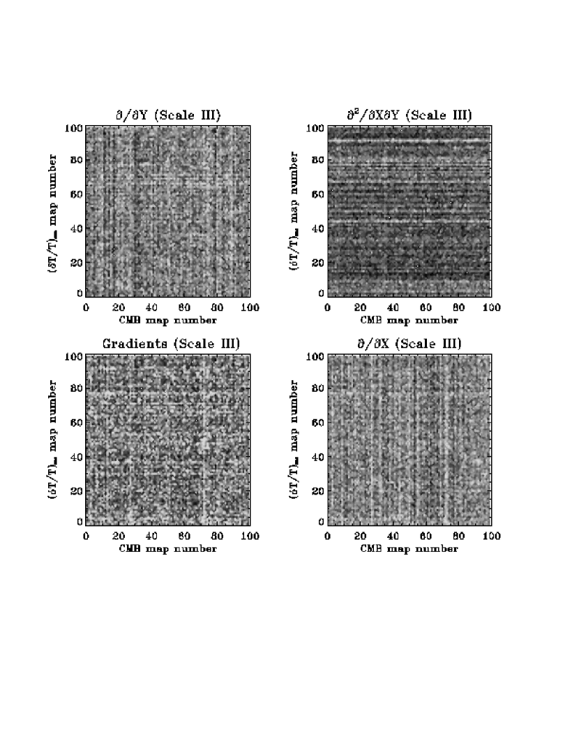
Figure 5: At the third decomposition scale, excess of kurtosis of $\partial/\partial x$, $\partial/\partial y$ and $\partial^{2}/\partial x\partial y$ coefficients, and multi-scale gradient coefficient. The $x$ and $y$ axes represent the number of maps. The studied secondary anisotropies are those due to both the inhomogeneous re-ionisation and the thermal and kinetic SZ effect + noise. The horizontal lines indicate the dominating non-gaussianity of the secondary anisotropies. The vertical lines exhibit the dominating primary CMB signal.

6 Effects of the instrumental configurations

We apply our statistical discriminators to test for non-gaussianity within the context of the representative instrumental configurations of the future MAP and Planck Surveyor satellite for CMB observations. The Planck configuration allows an investigation of the beam convolution effects alone, because the noise level remains unchanged. Whereas for the MAP configuration, we vary both the beam and the noise level.

6.1 MAP-like configuration

We have used a MAP-like instrumental configuration corresponding to a convolution, with a gaussian beam of full width at half maximum of 12 arcminutes, of maps consisting of the primary CMB anisotropies to which we added the secondary anisotropies. The noise added to the convolved maps is gaussian with $rms$ amplitude $(\delta T/T)_{rms}=10^{-5}$. From these “observed” maps, we compute the median excess of kurtosis for the multi-scale gradient coefficients and for the coefficients of the first and cross derivatives. At the first two decomposition scales the signal is suppressed due to the beam dilution effects and the fourth decomposition scale is dominated by the CMB primary anisotropies. In the MAP-like configuration, we are therefore left with a unique decomposition scale, the third, to test non-gaussianity using our methods. At this scale, the excess of kurtosis for the cross derivatives is $0.07\pm 0.03$. Whereas it is rather large for the multi-scale gradient, and first derivatives respectively, $1.15^{+2.24}_{-0.78}$ and $0.14^{+0.13}_{-0.10}$. Here again, the non-zero excess of kurtosis is possibly due to a sample variance problem, as the 12 arcminute convolution sharply cuts the power at the third decomposition level (Fig. 1). Using the PDF of the excess of kurtosis, we compute the probability that the measured excess belongs to a non-gaussian signal and we find it below the one sigma detection limit. We also apply the Kolmogorov-Smirnov (K-S) test (Press et al. 1992) which compares globally two distribution functions, especially the shift in the median value. We find that the PDFs of the gaussian process and of the “real sky” observed by MAP are identical. These results, using our statistical discriminators, thus suggest that the MAP satellite will be unable to detect non-gaussianity.

6.2 Planck Surveyor-like configuration

We use the same astrophysical contributions as those of the MAP-like configuration (primary and SZ + inhomogeneous re-ionisation secondary anisotropies). These maps are convolved with a 6 arcminutes gaussian beam. We also take into account the expected gaussian noise of Planck ($(\delta T/T)_{rms}\sim 2.\,10^{-6}$ per 1.5 arcminute pixel). The convolution by a 6 arcminute beam suppresses the power at the corresponding scale (Scale I) and affects the second decomposition scale. The third one is not significantly altered by the convolution and we expect that the non-gaussianity could thus be detected. For the multi-scale gradient we find $k=0.62^{+1.43}_{-0.60}$. Whereas we find for the first and cross derivatives respectively, $k=0.07^{+0.11}_{-0.08}$ and $0.16\pm 0.10$. In order to quantify the detectability of the non-gaussianity in the Planck-like configuration, we generate gaussian distributed maps with same power spectrum as the studied signal. We plot (Fig. 6) the PDF of the gaussian (dashed line) and non-gaussian (solid line) processes. We derive the probability that the median excess of kurtosis measured on the “real sky” belongs to the gaussian process. Using the multi-scale gradient we find that the probability of detecting non-gaussianity is 71.9% at the second decomposition scale. There is no significant detection elsewhere. Whereas using the cross derivative coefficients the probability of detecting a non-gaussian signature at the third scale is 94.5%. We apply the K-S test to the distribution of the excess of kurtosis for the cross derivative and find a probability of 96.6% of detecting non-gaussianity. Since the K-S test compares the two distributions, it is very sensitive to departures form gaussianity. It thus gives better results on the detection of the non-gaussian signature.

Figure 6: For the Planck-like configuration (CMB + SZ + inhomogeneous re-ionisation), probability distribution functions, as percentages, of the excess of kurtosis computed with the multi-scale gradient coefficients (right panels) and with the cross derivative coefficients (left panels). The dashed line is for the gaussian test maps with same power spectrum as the non-gaussian signal (solid line).

7 Discussion & Conclusion

The secondary anisotropies, due to CMB photon interactions, are superimposed on the primary anisotropies which are directly related to the seeds of the cosmic structures. The primary anisotropies can be gaussian distributed (inflationary models) or can exhibit an intrinsic non-gaussian signature (topological defect models). In the context of future CMB observations (high sensitivity, high resolution and large sky coverage), we will use the full information related to the CMB temperature anisotropies, in particular the statistical information, to distinguish between the two main cosmological models. Similarly, studies aiming at predicting and quantifying the foreground contributions to the temperature anisotropies have to characterise the non-gaussian foreground signals in order to subtract them before detailed CMB analysis.

In the present study we investigate the tests of non-gaussianity when this is induced by secondary anisotropies, the primary anisotropies being gaussian distributed. We study the effects arising from the interactions of the CMB photons and the ionised matter. More specifically, we focus on two effects which dominate all the other secondary effects of a scattering nature: the spatially inhomogeneous re-ionisation which peaks at scales of a few tens of arcminutes to one degree and the SZ effect which dominates at the few arcminutes scale. In order to search for non-gaussianity we use discriminators based on the study of the statistical properties of the coefficients in a four level wavelet decomposition (Forni & Aghanim 1999).

The primary anisotropies are gaussian at all scales. Nonetheless, we find a non-zero value of the multi-scale gradient excess of kurtosis, and hence first derivatives, at the second decomposition scale which could be misinterpreted as a non-gaussian signature. This can be understood in the following way: the window function of the wavelet at this scale (centred around $l\sim 2800$) encompasses the cut off in the angular power spectrum. As a result the corresponding sample variance induces a non-zero kurtosis for the multi-scale gradient coefficients. The presence of this non-zero value depends on the cosmological model as well as on the window filter that is the wavelet function. A similar non-zero value could exist at any decomposition scale where the CMB power spectrum has a sharp cut off. For the standard CDM model we use here, the cut off occurs at the second scale. In the case where the cosmological model has more power at small angular scales, or undergoes an overall shift of the spectrum towards large multipoles, the sample variance effects decrease. In the same way, we can use a wider wavelet which in turn decreases the sample effects. However, this attenuates the non-gaussian signature we search for. We apply a detection strategy proposed in Forni & Aghanim (1999), which allows the quantification of the detectability regardless of the power spectrum of the studied signal.

We have studied the case of secondary anisotropies induced by a spatially inhomogeneous re-ionisation of the Universe. Assuming that this was the only source of secondary anisotropies, we succeed in demonstrating its non-gaussian signature at the first and second decomposition scales. However, inhomogeneous re-ionisation is far from being the only source of anisotropies. The SZ effect due to galaxy clusters is known to be the most common source which is related to the CMB photon scattering off free electrons. In this study, we also take into account the SZ effect of a predicted cluster population which we add to the primary CMB fluctuations and to the re-ionisation anisotropies. The non-gaussian foreground model is a worst case example because we do not remove any foregrounds. Owing to its peculiar spectral signature the thermal effect is expected to be removed from the cosmological signal (temperature anisotropies). However, the subtraction is not complete because almost 1/5 of the SZ effect contribution is due to the kinetic SZ effect, which is spectrally indistinguishable from the primary anisotropies, and there remains a significant non-gaussian foreground contribution. In our study, we find that the dominant non-gaussian signal is due to the SZ effect of clusters. The non-gaussian signature is found to be orders of magnitude larger than in the case without the SZ contribution and we clearly detect the non-gaussianity. The strong non-gaussian signature, associated with the SZ effect, comes from the gas profile of individual clusters. We have analysed temperature anisotropy maps with different profiles (gaussian, $\beta$ profiles or even so point-like sources) to which we add the primary gaussian anisotropies. As it is very peaked at the centre, the cluster induces a sharp variation in the signal from the center to the outskirts of the structure. In addition, an important fraction of the cluster population is composed of unresolved point-like clusters. We thus find that clusters represent the dominant non-gaussian foreground.

We apply our statistical tests to Planck-like and MAP-like instrumental configurations in order to compare the capabilities of the two planned satellites for detecting the non-gaussian signature induced by the secondary anisotropies (mainly the SZ effect). For both configurations the fourth, and largest scale, shows no significant non-gaussianity due to the SZ contribution. In the MAP-like configuration the beam convolution affects the first two decomposition scales. Therefore, we are only left with the third scale to search for non-gaussianity. At the same time, the convolution rather sharply reduces the contributions at angular scale associated with the third decomposition level. This induces a non-zero excess of kurtosis. We apply our detection strategy to overcome the problem and avoid a possible misinterpretation on non-gaussianity. We find no significant detection of the non-gaussian signature at the third scale for the MAP-like configuration. By contrast, for the Planck-like configuration, we detect the non-gaussian signature at the third decomposition scale, the first and second ones being affected by the beam convolution.

We have shown that our statistical tests combined with a detection strategy based on the characterisation of gaussian test maps, with same power spectrum as the non-gaussian studied process, are appropriate tools for demonstrating a non-gaussian signature. In a forthcoming paper, we will search for other discriminatory methods that allow two (or more) non-gaussian signals to be distinguished, in order to subtract the non-gaussian signature of the secondary anisotropies from the non-gaussian signature of the primary fluctuations.