Abstract

We consider the deconvolution of the thermal and the turbulent profiles for a pair of ions with different atomic weights under the condition that the lines are formed in an absorbing medium with fluctuating density and velocity fields. Our method is based on the entropy-regularized $\chi^{2}$-minimization (ERM) procedure. From synthetic spectra we found that the CII and SiII lines can be used to estimate the mean (density weighted) kinetic temperature with a sufficiently high accuracy ($\sim$ 10%) in a rather wide range of the ionization parameter, $-6.0\;\raise 1.29167pt\hbox{$<$\kern-7.5pt\raise-4.73611pt\hbox{$\sim$}}\;\log U\;\raise 1.29167pt\hbox{$<$\kern-7.5pt\raise-4.73611pt\hbox{$\sim$}}\;-2.0$. This is a generalization of a previous result [5] where we did not account for density fluctuations.

ON THE MEASUREMENT OF KINETIC TEMPERATURE IN HIGH REDSHIFT GALACTIC HALOS

¹ Department of Theoretical Astrophysics, Ioffe Institute, St.Petersburg, Russia. ² Institut für Theoretische Physik der Universität Frankfurt am Main, Frankfurt/Main, Germany.

1 Introduction

One of the main source of information about the physical properties of the intergalactic gas is the study of metal-line absorption in quasar spectra. Metal lines in the Lyman Limit Systems (LLS), – i.e. in systems with $N_{\rm HI}\;\raise 1.29167pt\hbox{$<$\kern-7.5pt\raise-4.73611pt\hbox{$\sim$}}\;2\times 10^{17}$ cm^-2 which are optically thin in the Lyman continuum, – are of particular interest in this regard because the Lyman continuum opacity does not affect the metal abundance measurements in this case [1]. Besides the LLSs often show carbon and silicon line absorption from different ionization states which allows estimating the ionization parameter $U$ (the ratio of the number of photons with energies above one Rydberg to the number of atoms, $U=n_{\gamma}/n_{\rm H}$).

The LLSs are usually assumed to arise in the outer regions of intervening galactic halos where the electron density is rather low, $n_{e}\sim 10^{-2}-10^{-3}$ cm^-3. For such tenuous gas the collisional ionization is not important in determining the ionization fractions of ions since typical kinetic temperatures for the gas showing absorption in CII – CIV lines and in SiII – SiIV lines are of the order $10^{4}-2\times 10^{4}$ K. It follows, that the outer parts of galactic halos are mainly photoionized and that the thermal and the ionization state of the gas may be specified by the ionization parameter $U$ only, [1]. Thus, for a given value of $n_{\gamma}$ (or the specific radiation flux $J_{0}$ at 1 Rydberg), the dispersion of $U$ along the line of sight represents a varying gas density.

In recent years, great efforts have been made towards the precise measurements of metal line profiles in QSO spectra obtained with high spectral resolution, FWHM $\sim 5-7$ km s^-1. However, current theoretical models cannot give a complete prediction to match the observational data [2].

The observations often show complex structures of the line profiles. It is traditional to treat them using the standard Voigt fitting deconvolution procedure. This procedure is based on the assumption that the apparent fluctuations within the line profile are caused by density clumps (‘cloudlets’) with different radial velocities. The non-thermal (turbulent) velocity field inside each cloudlet is accounted for in the so-called microturbulent approximation. It was shown in [3], however, that the microturbulent analysis may produce unphysical kinetic temperatures.

The more general mesoturbulent approach (see [4] and the references cited therein) is based on the assumption that the intensity fluctuations within the line profile arise mainly from the irregular Doppler shifts in the absorption coefficient caused by macroscopic large-scale, rather than thermal, motions. If the macroscopic velocity field has a correlation length not small as compared with the linear size of the absorbing region, then the radial velocity distribution may deviated significantly from the Gaussian model.

In a previous paper [5] we developed a method aimed at recovering the kinetic temperature from complex metal-line spectra assuming a homogeneous gas density and a random velocity field. Here we outline our first results for the case when both the density and the velocity fields are of random nature.

2 The ERM procedure and results

The entropy-regularized $\chi^{2}$-minimization (ERM) procedure utilizes complex but similar absorption line profiles of ions with different atomic weights to estimate the mean value of $T_{\rm kin}$ for the whole absorbing region. The similarity of the complex profiles of ions with different masses and ionization potentials stems from the equal ionization fraction for both of them. To illustrate this statement we used a model thoroughly described in [1] : an optically thin gas ionized by a typical QSO photoionizing spectrum [6] with the metallicity ${\rm Z}/{\rm Z}_{\odot}=0.1$.

The consequent steps of our computational experiment are shown in Fig. 1. Panel (a) presents the random velocity field $u(x)=v(x)/\sigma_{\rm turb}$, where $x$ is the space coordinate $s$ along the line of sight in units of the linear size $L$ of the absorbing region. The fluctuating density field $n(x)/n_{0}$ is depicted in panel (b). Both the velocity and the gas density fields were calculated using the moving average method described in [5]. To obtain the real gas density fluctuations, we used the log-normal distribution for the density contrast $\delta=(n-n_{0})/n_{0}$ with the rms value of $\sigma_{\delta}=1$ and $n_{0}=2\times 10^{-3}$ cm^-3. The rms value for the velocity field was assumed to be 20 km s^-1, and the linear size of the region $L=5$ kpc. The chosen specific radiation flux $J_{0}=5\times 10^{-22}$ ergs cm^-2 s^-1 Hz^-1 corresponds in our case to $U_{0}=1.3\times 10^{-3}$. In panel (c) we plot the equilibrium kinetic temperature $T_{4}(x)$ in units $10^{4}$ K as a function of the ionization parameter $U(x)$ in accord with the numerical results [1]. The fluctuations of $U(x)$ are shown in panel (d). For each species we calculated the density weighted mean temperature

$$\langle T\rangle=\frac{\int n_{\rm ion}(s)\,T(s)\,ds}{\int n_{\rm ion}(s)\,ds}\>.$$ (1)

The corresponding values of $\langle T\rangle$ we find for CII, SiII, CIV, and SiIV are 15120 K, 15140 K, 17120 K, and 16390 K, respectively.

These random fields lead in turn to complex profiles of CII$\lambda 1334$, SiII$\lambda 1260$, CIV$\lambda 1548$, and SiIV$\lambda 1394$. All profiles have been convolved with a Gaussian spectrograph function having the width of 7 km s^-1 (FWHM), and then a Gaussian noise of S/N = 75 has been added. The final patterns are shown in panels (e), (f), (g), and (h), respectively, by dots with corresponding error bars.

It is seen that the CII and SiII profiles are similar whereas the intensity fluctuations within the CIV profile differ from those for the SiIV line. This different behavior of low and high ionized species formed in the same absorbing region is clearly illustrated in panel (i). The ratio of fractional ionization for the CII and SiII lines is almost constant over the whole range of $U$-values, but the corresponding ratio for the CIV and SiIV lines is highly sensitive to the variation of $U$.

Next we considered these spectra as ‘observed’ and analyzed them in two ways. At first we applied the standard Voigt profile fitting procedure. The results are shown in Figures 1e–1h, in where the individual components are indicated by tick marks and the numbers give the corresponding parameters (the first line gives the column density, the second the $b$ parameter. In Fig. 1h the third line gives the derived temperature). The smooth curves show the resulting ‘theoretical’ profiles. We see that the derived temperatures vary between 2800 K and 45900 K whereas the input temperature (Fig. 1c) varies only between 14360 K and 22090 K. Contrary, when we apply our new ERM procedure [5] to the CII and SiII lines we find from Fig. 1j (shaded area) a temperature of $15200\pm 200$ K. This value is in good agreement with the density averaged temperatures derived before.

This result reinforces our previous finding that the Voigt profile fitting procedure may lead to unphysical temperatures. On the other side it indicates that – at least for the cases studied so far – our new procedure gives a physically reasonable average value of the kinetic temperature.

This is a report on work in progress.

Acknowledgment. This work has been supported by the Deutsche Forschungsgemeinschaft. SAL thanks the conference organizers for financial assistance.

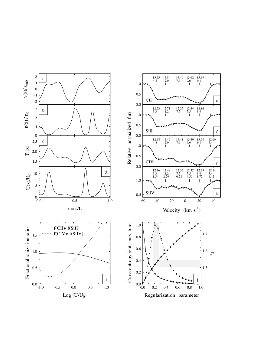
Figure 1: An example of Monte-Carlo simulations. ($a$) One realization of the stochastic velocity field ($\sigma_{\rm turb}=20$ km s^-1), ($b$) the density field ($n_{0}=0.002$ cm^-3), ($c$) the kinetic temperature field (in units $10^{4}$ K), and ($d$) the ionization parameter field ($U_{0}=1.3\times 10^{-3}$) versus the normalized space coordinate. ($e,f,g,h$) Velocity plots of the simulated spectra (dots and $1\sigma$ error bars) and the Voigt profile fits to the CII, SiII, CIV, and SiIV lines (smooth curves). The column density and velocity dispersion are displayed on top of each line. The third line in panel ($h$) shows the derived temperature for each subcomponent. ($i$) Fractional ionization ratios for the pair CII/SiII and CIV/SiIV lines versus the normalized ionization parameter. ($j$) The normalized cross-entropy (filled circles connected by smooth line), its curvature (dotted line), and the kinetic temperature (dashed line) versus the normalized regularization parameter $\hat{\alpha}$ (for more details see [5]). The shaded area restricts the region of optimal values of $\hat{\alpha}$ and corresponding solutions for $T_{\rm kin}$.

References

- [1] Donahue M., Shull M., 1991, Astrophys. J. 383, 511
- [2] Kirkman D., Tytler D. 1999, Astrophys. J. 512, L5
- [3] Levshakov S. A., Kegel W. H., Mazets I. E., 1997, MNRAS 288, 802
- [4] Levshakov S. A., Kegel W. H., Takahara F., 1999, MNRAS 302, 707
- [5] Levshakov S. A., Takahara F., Agafonova I. I., 1999, Astrophys. J. 517, in press
- [6] Mathews W. D., Ferland G., 1987, Astrophys. J. 323, 456