Searching for non-gaussianity: Statistical tests

Abstract

Non-gaussianity represents the statistical signature of physical processes such as turbulence. It can also be used as a powerful tool to discriminate between competing cosmological scenarios. A canonical analysis of non-gaussianity is based on the study of the distribution of the signal in the real (or direct) space (e.g. brightness, temperature).

This work presents an image processing method in which we propose statistical tests to indicate and quantify the non-gaussian nature of a signal. Our method is based on a wavelet analysis of a signal. Because the temperature or brightness distribution is a rather weak discriminator, the search for the statistical signature of non-gaussianity relies on the study of the coefficient distribution of an image in the wavelet decomposition basis which is much more sensitive.

We develop two statistical tests for non-gaussianity. In order to test their reliability, we apply them to sets of test maps representing a combination of gaussian and non-gaussian signals. We deliberately choose a signal with a weak non-gaussian signature and we find that such a non-gaussian signature is easily detected using our statistical discriminators. In a second paper, we apply the tests in a cosmological context.

1 Introduction

Non-gaussianity is a very promising way of characterising some important physical processes and has many applications in astrophysics. In fluid mechanics, the non-gaussian signature of the probability density functions of velocity is used as evidence for turbulence (e.g. Chabaud et al. (1994)). Astrophysical fluids with very large Reynolds numbers, such as the interstellar medium, are expected to be turbulent. If it exists, turbulence should play a leading role in the triggering of star formation, in determining the dynamical structure of the interstellar medium and its chemical evolution. Non-gaussianity is a tool for indicating turbulence. Indeed, recent studies on the non-gaussian shape of the molecular line profiles can be interpreted as evidence for turbulence (Falgarone & Phillips 1990; Falgarone et al. 1994; Falgarone & Puget 1995; Miville-Deschênes et al. 1999). Non-gaussianity is also used as the indicator of coronal heating due to magneto-hydro-dynamical turbulence (Bocchialini et al. 1997; Georgoulis et al. 1998). Within the cosmological framework, the statistical nature of the Cosmic Microwave Background (CMB) temperature, or brightness anisotropies, probes the origin of the initial density perturbations which gave rise to cosmic structures (galaxies, galaxy clusters). The inflationary models (Guth 1981; Linde 1982) predict gaussian distributed density perturbations, whereas the topological defect models (Vilenkin 1985; Bouchet 1988; Stebbins 1988; Turok 1989) generate a non-gaussian distribution. Because the nature of the initial density perturbations is a major question in cosmology, a lot of statistical tools have been developed to test for non-gaussianity.

In order to test for non-gaussianity, one can use traditional methods based on the distribution of temperature anisotropies. The simplest tests are based on the third and/or fourth order moments (skewness and kurtosis) of the distribution, both equal to zero for a gaussian distribution. Another test for non-gaussianity through the temperature distribution is based on the study of the cumulants (Ferreira et al 1997; Winitzki 1998). The n-point correlation functions also give very valuable statistical information. In particular, the three-point function, and its spherical harmonic transform (the bispectrum), are appropriate tools for the detection of non-gaussianity (Luo & Schramm 1993; Kogut et al. 1996; Ferreira & Magueijo 1997; Ferreira et al. 1998; Heavens 1998; Spergel & Goldberg 1998). An investigation of the detailed behaviour of each multipole of the CMB angular power spectrum (transform of the two-point function) is another non-gaussianity indicator (Magueijo 1995). Finally, other tests of non-gaussianity are based on topological pattern statistics (Coles 1988; Gott et al. 1990).

The works of Ferreira & Magueijo (1997) on the search for non-gaussianity in Fourier space, and of Ferreira et al. (1997) on the cumulants of wavelet transformed maps, have shown that these approaches allow the study of characteristic scales, which is particularly interesting when studying a combination of gaussian and non-gaussian signals as a function of scale. In the present work, we study non-gaussianity in a wavelet decomposition framework, that is, using the coefficients in the wavelet decomposition. We decompose the image of the studied signal into a wavelet basis and analyse the statistical properties of the coefficient distribution. We then search for reliable statistical diagnoses to distinguish between gaussian and non-gaussian signals. The aim of this study is to find suitable tools for demonstrating and to quantifying the non-gaussian signature of a signal when it is combined with a gaussian distributed signal of similar, or higher, amplitude.
In section 2, we describe the methods for wavelet decomposition and filtering. We then briefly describe the characteristics of the wavelet we use in our study. We also give the main characteristics of the test data sets used in our work. In section 3, we present the statistical criteria we developed to test for non-gaussianity. We then apply the tests to sets of gaussian test maps (Sec. 4). We also apply them, in section 5, to sets of non-gaussian maps as well as combinations of gaussian and non-gaussian signals with the same power spectrum. In section 6, we present and apply the detection strategy we propose to quantify the detectability of the non-gaussian signature. Finally, in section 7 we conclude and present our main results.

2 Analysis

2.1 The wavelet decomposition

Wavelet transforms have been widely investigated recently because of their suitability for a large number of signal and image processing tasks. Wavelet analysis involves a convolution of the signal with a convolving function or a kernel (the wavelet) of specific mathematical properties. When satisfied, these properties define an orthogonal basis, which conserves energy, and guarantee the existence of an inverse to the wavelet transform.

The principle behind the wavelet transform, as described by Grossman & Morlet (1984), Daubechies (1988) and Mallat (1989), is to hierarchically decompose an input signal into a series of successively lower resolution reference signals and their associated detail signals. At each decomposition level, L, the reference signal has a resolution reduced by a factor of $\mathrm{2^{L}}$ with respect to the original signal. Together with its respective detail signal, each scale contains the information needed to reconstruct the reference signal at the next higher resolution level. Wavelet analysis can therefore be considered as a series of bandpass filters and be viewed as the decomposition of the signal into a set of independent, spatially oriented frequency channels. Using the orthogonality properties, a function in this decomposition can be completely characterised by the wavelet basis and the wavelet coefficients of the decomposition.

The multilevel wavelet transform (analysis stage) decomposes the signal into sets of different frequency localisations. It is performed by iterative application of a pair of Quadrature Mirror Filters (QMF). A scaling function and a wavelet function are associated with this analysis filter bank. The continuous scaling function $\phi_{A}(x)$ satisfies the following two-scale equation:

$$\phi_{A}(x)=\sqrt{2}\sum_{n}h_{0}(n)\phi_{A}(2x-n),$$ (1)

where $\mathrm{h_{0}}$ is the low-pass QMF. The continuous wavelet $\psi_{A}(x)$ is defined in terms of the scaling function and the high-pass QMF $\mathrm{h_{1}}$ through:

$$\psi_{A}(x)=\sqrt{2}\sum_{n}h_{1}(n)\phi_{A}(2x-n).$$ (2)

The same relations apply for the inverse transform (synthesis stage) but, generally, different scaling function and wavelet ($\phi_{S}(x)$ and $\psi_{S}(x)$) are associated with this stage:

$$\phi_{S}(x)=\sqrt{2}\sum_{n}g_{0}(n)\phi_{S}(2x-n),$$ (3)

$$\psi_{S}(x)=\sqrt{2}\sum_{n}g_{1}(n)\phi_{S}(2x-n).$$ (4)

Equations (1) and (3) converge to compactly supported basis functions when

$$\sum_{n}h_{0}(n)=\sum_{n}g_{0}(n)=\sqrt{2}.$$ (5)

The system is said to be biorthogonal if the following conditions are satisfied:

$$\int_{\mathbb{R}}\phi_{A}(x)\phi_{S}(x-k)dx=\delta(k)$$ (6)

$$\int_{\mathbb{R}}\phi_{A}(x)\psi_{S}(x-k)dx=0$$ (7)

$$\int_{\mathbb{R}}\phi_{S}(x)\psi_{A}(x-k)dx=0$$ (8)

Cohen et al. (1990) and Vetterli & Herley (1992) give a complete treatment of the relationship between the filter coefficients and the scaling functions.

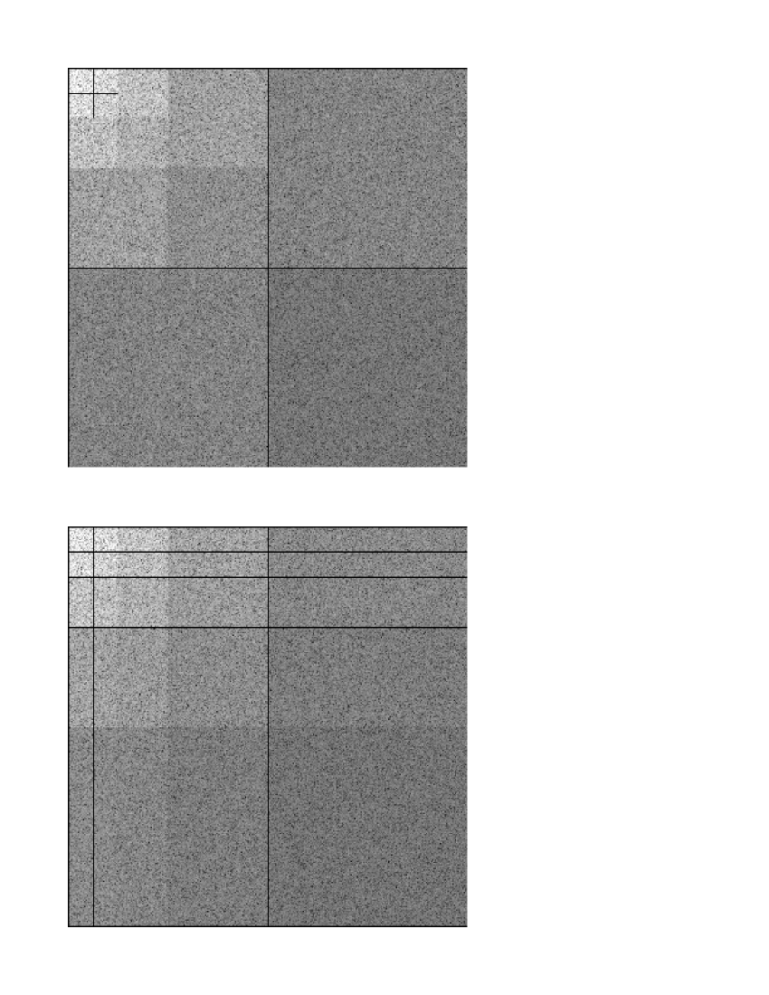
Figure 1: In the upper panel, a 4 level “dyadic” decomposition is used, in the lower, a 4 level “pyramidal” decomposition is used. In both cases, the diagonal squares and the last decomposition level are identical and the grey levels indicate the amplitude of the wavelet coefficients.

When applied to bi-dimensional data (typically images), three main types of decomposition can be considered: dyadic (or octave band), pyramidal and uniform.

1. A “dyadic” decomposition refers to a transform in which only the reference sub-band (low-pass part of the signal) is decomposed at each level. In this case, the analysis stage is applied in both directions of the image at each decomposition level. The total number of sub-bands after L levels of decomposition is then 3L+1 (Fig. 1, upper panel).

2. A “pyramidal” decomposition is similar to a “dyadic” decomposition in the sense that only the reference sub-band is decomposed at each level, but it refers here to a transform that is performed separately in the two directions of the image. The total number of sub-bands after L levels of decomposition is then $\mathrm{(L+1)^{2}}$ (Fig. 1, lower panel).

3. A “uniform” decomposition refers to one in which all sub-bands are transformed at each level. The total number of sub-bands after L levels of decomposition is then $\mathrm{4^{L}}$.

The wavelet functions are localised in space and, simultaneously, they are also localised in frequency. Therefore, this approach is an elegant and powerful tool for image analysis because the features of interest in an image are present at different characteristic scales. Moreover, if the input field is gaussian distributed, the output is distributed the same way, regardless of the power spectrum. This arises from the linear transformation properties of gaussian variables. The distribution of the wavelet coefficients of a gaussian process is thus a gaussian. Conversely, we expect that any non-gaussian signal will exhibit a non-gaussian distribution of its wavelet coefficients.

In our study, we have used bi-orthogonal wavelets, which are mainly used in data compression, because of their better performance than orthogonal wavelets, in compacting the energy into fewer significant coefficients. There exist bi-orthogonal wavelet bases of compact support that are symmetric or antisymmetric. Antisymmetric wavelets are proportional to, or almost proportional to, a first derivative operator (e.g. the 2/6 tap filter (filter #5) of Villasenor et al. (1995), or the famous Haar transform which is an orthogonal wavelet). Symmetric wavelets are proportional to, or almost proportional to, a second derivative operator (e.g. the 9/3 tap filter of Antonini et al. (1992)). In the frame of detecting non-gaussian signatures, the choice of the wavelet basis is critical because non gaussian features exhibit point sources or step edges the wavelet must have a very good impulse response and a low shift variance, i.e. they better preserve the amplitude and the location of the details. Villasenor et al. (1995) have tested a set of bi-orthogonal filter banks, within this context, to determine the best ones for image compression. They conclude that even length filters have significantly less shift variance than odd length filters, and that their performance in term of impulse response is superior. In these filters, the high pass QMF is antisymmetric which is also a desirable property in the sense that we will also be interested in the statistical properties of the multi-scale gradients. Consequently, in our study, we have chosen the 6/10 tap filter (filter #3) of Villasenor et al. (1995) (Fig. 2) which represents the best compromise between all the criteria and energy compaction. Using this filter, we have chosen to perform a four level dyadic decomposition of our data. This particular wavelet and decomposition method have already been used for source detection by Aghanim et al. (1998).

Figure 2: Scaling function (top) and wavelet function (bottom) corresponding to the filter #3 of Villasenor et al. (1995). Note that the wavelet function is antisymmetric.

With such a decomposition, we also benefit from correlations between the two directions at each level, which is not the case with the pyramidal decomposition that treats both directions as if they were independent. Another advantage of this transform is that, for each level of decomposition, or scale, we benefit from the maximum number of coefficients possible, which is crucial for the statistics.

2.2 The test maps

We use a test case which consists of sets of 100 maps of a gaussian signal and 200 maps of a non-gaussian signal, all having the same bell-shaped power spectrum and $512\times 512$ pixels. One of the non-gaussian sets (100 maps) consists of a distribution of disks with uniform amplitude (top-hat profiles), generating step edges. The disks have different sizes and amplitudes and are randomly distributed in the map. The signal is weakly skewed because the average skewness, which is the third moment of the distribution, computed over the 100 non-gaussian realisations is $\mu_{3}=-0.10\pm 0.05$ (one sigma error for one realisation). Whereas the excess of kurtosis, the fourth moment ($\mu_{4}$) of the distribution, is $k=\mu_{4}/\mu_{2}^{2}-3=1.09\pm 0.17$. The second set of 100 non-gaussian maps consists of a distribution of gaussian profiles with different sizes and amplitudes. The skewness and excess of kurtosis of the 100 statistical realisations of the non-gaussian distribution of gaussian profiles are respectively $-0.06\pm 0.04$ and $1.19\pm 0.13$. The same quantities computed over the 100 gaussian maps are respectively $\mu_{3}=0.14\,10^{-2}\pm 2.15\,10^{-2}$ and $0.03\,10^{-2}\pm 3.87\,10^{-2}$. These numbers should be equal to zero for a gaussian distribution. They are not because there is a statistical dispersion over a finite set of realisations. The purpose of this paper being to develop suitable statistical tests for non-gaussianity, we will not study other effects such as noise or beam dilution. These effects will be considered in an application of the method to the CMB signal in a second paper (Aghanim & Forni 1999).

3 Tests of non-gaussianity

The most direct and obvious way of analysing the statistical properties of an image is to use the distribution of the pixel brightnesses, or temperatures, together with the skewness and kurtosis. If the two quantities are different from zero, they indicate that the signal is non-gaussian. However, a weak non-gaussian signal will hardly be detected through the moments of the temperature distribution. Another way of addressing the problem is to use the coefficients in the wavelet decomposition and to study their statistical properties which in turn characterise the signal. In fact, the wavelet coefficients are quite sensitive to variations (even weak ones) in the signal, temperature or brightness, and hence to the statistical properties of the underlying process. We have developed two tests which exhibit the non-gaussian characteristics of a signal using the wavelet coefficients. Since our test maps are not skewed in the following we focus only on the results obtained using the fourth moment.

For the first discriminator, we study the statistical properties of the distribution of the multi-scale gradient coefficients. This method is appropriate when dealing with a non-gaussian process characterised by sharp edges and consequently by strong gradients in the signal. Indeed, in any region where the analysed function is smooth the wavelet coefficients are small. On the contrary, any abrupt change in the behaviour of the function increases the amplitude of the coefficients around the singularity. The detection of non-gaussianity is thus based on the search of these gradients. In the dyadic wavelet decomposition one can discriminate between the coefficients associated with vertical and horizontal gradients and the other coefficients. In our case, the vertical and horizontal gradients are analogous to the partial derivatives, $\partial/\partial x$ and $\partial/\partial y$, of the signal. Mallat & Zhong (1992) give a thorough treatment of the characterisation of signals from multi-scale edges. We compute the quadratic sum of the coefficients, the quantity ${\mathcal{G}}_{L}=\left(\partial/\partial x\right)_{L}^{2}+\left(\partial/\partial y\right)_{L}^{2}$, at each decomposition level $L$. This quantity represents the squared amplitude of the multi-scale gradient of the image. In the following, we will however refer to it as the multi-scale gradient coefficient.

The second statistical discriminator is based on the study of the wavelet coefficients related to the horizontal, vertical and diagonal gradients. These coefficients are associated with the partial derivatives $\partial/\partial y$ and $\partial/\partial x$, as in the multi-scale gradient method, as well as with the cross derivative $\partial^{2}/\partial x\partial y$. The coefficients are computed at each decomposition level and their excess of kurtosis with respect to a Gauss distribution exhibits the non-gaussian signature of the studied signal. In this context, the wavelet coefficients associated with the first derivatives are obviously closely related to the multi-scale gradient.
In the following, we first apply our two tests to purely gaussian and non-gaussian maps. We then test the detectability of a non-gaussian signal added to a gaussian one with same power spectrum and with increasing mixing ratios.

4 Characterisation of gaussian signals

4.1 The multi-scale gradient and its distribution

For the 100 gaussian maps, we find that the histogram of the multi-scale gradient coefficients can be fitted by the positive wing of the Laplace probability distribution function:

$${\mathcal{H}}({\mathcal{G}}_{L})=\frac{1}{\sqrt{2}\,\sigma}\,\exp\left(-\frac{\sqrt{2}\,({\mathcal{G}_{L}}-\mu_{1})}{\sigma}\right),$$ (9)

where $\mu_{1}$ is the mean of the distribution (theoretically equal to zero) and $\sigma^{2}$ is its second moment.

Figure 3: Fits of the multi-scale gradient coefficient histograms obtained with the 100 statistical realisations. In all plots, the error bar is for one realisation. The left panels are given for the gaussian process whereas the right panels represent the non-gaussian signal. The wings at large multi-scale gradient indicate the non-gaussian signature.

We plot in figure 3 (left panels) the distribution of the multi-scale gradient coefficients in the four decomposition scales for the gaussian signal. For reasons of legibility, we have just plotted the fit obtained with the 100 maps. The error bars represent a confidence interval (for one realisation) and account for the statistical dispersion of the realisations.

We can analyse the multi-scale gradient distribution through its $n$th-order moments ($\mu_{n}$). In particular, we compute the excess of kurtosis using the second and fourth moments of the distribution($\mu_{2}$ and $\mu_{4}$). For a gaussian distribution, the normalised excess is zero. For a Laplace distribution, the fourth moment is given by $\mu_{4}=6\mu_{2}^{2}$. The normalised excess of kurtosis $k=\mu_{4}/\mu_{2}^{2}-6$ highlights the non-gaussian signature of a signal through the departure of the multi-scale gradient from a Laplace distribution.

At each decomposition level, we compute the normalised excess of kurtosis of the multi-scale gradient coefficients for the 100 gaussian maps, and we derive a representative value of the distribution that is the mean $\overline{k}$ which we quote in Table 1. The results show that $\overline{k}$ is very close to zero. The $\sigma$ values correspond to the root mean square values with respect to the mean $\overline{k}$. The $\sigma$ values define a confidence interval, or a probability distribution of the excess of kurtosis. For the gaussian signal the upper and lower boundaries of this interval are equal suggesting that the $k$ values are gaussian distributed. The increasing $\sigma$ (Fig. 3, left panels) with the decomposition scale is due to the larger dispersion. This feature is also the consequence of the smaller number of wavelet coefficients at higher decomposition scales.

Scale	$\overline{k}$	$\sigma_{\pm}$
I	0.04	0.15
II	0.05	0.32
III	-0.01	0.51
VI	-0.006	0.869

Table 1: The mean excess of kurtosis at four decomposition scales computed over the 100 gaussian maps. The $\sigma_{\pm}$ values define the confidence intervals for one realisation.

4.2 Partial derivatives

	Scale	$\overline{k}_{1}$	$\sigma_{\pm}$		$\overline{k}_{2}$	$\sigma_{\pm}$
	I	0.010	0.020		0.003	0.022
$\partial/\partial x$	II	0.012	0.043	$\partial^{2}/\partial x\partial y$	0.005	0.042
&	III	-0.001	0.079		0.006	0.072
$\partial/\partial y$	VI	0.006	0.150		0.018	0.014

Table 2: The mean excess of kurtosis at four decomposition scales. $\overline{k}_{1}$ is computed using the wavelet coefficients associated with $\partial/\partial x$ and $\partial/\partial y$. $\overline{k}_{2}$ is computed using the coefficients of $\partial^{2}/\partial x\partial y$. The $\sigma_{\pm}$ values define the confidence intervals for one realisation.

Figure 4: Excess of kurtosis computed over the wavelet coefficients of respectively $\partial/\partial x$ for the left panels, $\partial/\partial y$ for the centre panels and $\partial^{2}/\partial x\partial y$ for the right panels. The solid line is for the non-gaussian process. The dashed line is for the gaussian process with same power spectrum.

The wavelet coefficient distributions associated with the first and cross derivatives are gaussian for the gaussian maps. We thus compute the normalised excess of kurtosis with respect to a gaussian distribution ($k=\mu_{4}/\mu_{2}^{2}-3$). These values are displayed in figure 4 (dashed line) for the gaussian maps. In this figure and at each decomposition scale, the first set of 100 values stands for the excess of kurtosis of the wavelet coefficients associated with the horizontal gradient ($\partial/\partial y$). The second set of 100 values represents the same quantity computed for the vertical gradient ($\partial/\partial x$) and the last one represents the excess of kurtosis for the wavelet coefficients associated with cross derivative $\partial^{2}/\partial x\partial y$ (diagonal gradients). We note that for the gaussian maps the excess is always centred around zero at all the decomposition scales. For the multi-scale gradient, the dispersion around the mean $\overline{k}$ increases with increasing decomposition scale. In table 2, we quote the mean together with the confidence intervals at each scale. The results also show that the values are close to zero confirming the gaussian nature of the signal.

As a result, we conclude that a gaussian signal can be characterised by the distribution of the multi-scale gradient coefficients and of the coefficients associated with $\partial/\partial x$, $\partial/\partial y$ and $\partial^{2}/\partial x\partial y$. In the first case, the multi-scale gradient coefficient distribution is fitted by a Laplace distribution and the excess of kurtosis is zero. In the second case, the excesses of kurtosis are gaussian distributed with $\overline{k}=0$ for the first and the cross derivatives.

We check these two characteristics on other gaussian processes with different power spectra. For a white noise spectrum, we find identical results as in the study case: zero excess of kurtosis for the multi-scale gradient and the coefficients of the partial derivatives. Since our statistical tests are based on the statistics of the wavelet coefficients at each decomposition scale, we expect that a sharp cut off in the power spectrum of the gaussian signal will induce a sample variance problem. We check this behaviour using a gaussian process exhibiting a very sharp cut off with a shape close to a Heaviside function, at the second decomposition scale. This cut off is similar to the cut off expected in the CMB power spectrum in a standard cold dark matter model. At all the decomposition scales except the second, we find the expected zero excess of kurtosis for the wavelet coefficients of gaussian signals. At the second decomposition scale, we find a non-zero excess of kurtosis for the multi-scale gradient coefficients, as well as for the coefficients related to the first derivatives, which could be misinterpreted for a non-gaussian signature. This non-zero excess has nothing to do with an intrinsic property of the studied signal, as the latter is gaussian at all scales. It comes from the very sharp decrease in power combined with the narrow filter associated with the wavelet basis. In fact, the contribution of the gaussian process, at this scale, is sparse. Therefore, it induces a sample variance effect which in turn results in a non-zero excess of kurtosis. We tested a wider filtering wavelet and found that the excess of kurtosis decreases. Nevertheless, a wider filtering wavelet smoothes the non-gaussian signatures and reduces the efficiency of our discriminating tests. However, at the second decomposition scale, the wavelet coefficients associated with $\partial^{2}/\partial x\partial y$ exhibit no excess of kurtosis for a process with sharp cut off. This indicates that the excess of kurtosis computed using the cross derivative coefficients is more reliable in characterising a gaussian process, and consequently non-gaussianity, regardless of the power spectrum.

We also analysed the sum of gaussian signals. When there is no cut off in the power, the excess of kurtosis for the sum of gaussian signals is zero for both discriminators. By contrast, if one of the gaussian signals presents a cut off at any decomposition scale, we again find a non-zero excess of kurtosis at the corresponding scale.

5 Application to non-gaussian signals

We apply our statistical discriminators to detect the non-gaussian signature of different processes. We first study two sets of non-gaussian maps, one constituted of a distribution of top-hat profiles and the other constituted of a distribution of gaussian profiles, both having the same power spectrum as the gaussian test maps used in the previous section. We also apply the statistical test to a combination of gaussian and non-gaussian signals with different mixing ratios.

5.1 The multi-scale gradient and its distribution

We compute the multi-scale gradient coefficients (${\mathcal{G}}_{L}$) using 100 statistical realisations of the non-gaussian process (top-hat profiles). At the four decomposition scales, we plot the fitted histogram (right panels of Figure 3). We note that the distribution of the multi-scale gradient coefficients also fits a Laplace distribution for small values of ${\mathcal{G}}_{L}$. However, there is a significant departure from this distribution for higher values. This is exhibited by the larger error bars and by the wings of the gradient distribution at large ${\mathcal{G}}_{L}$. Figure 3 (right panels) exhibits the non-gaussian signatures mostly at the first three decomposition scales. At the fourth, the lack of coefficients enlarges the error bars but we still marginally distinguish the non-gaussian signal.

Scale	$k_{1}$	$\sigma_{+}$	$\sigma_{-}$	$k_{2}$	$\sigma_{+}$	$\sigma_{-}$
I	14.50	35.38	5.06	1.5	0.51	0.27
II	3.87	2.68	0.77	1.9	1.43	0.48
III	3.54	2.17	1.24	3.46	2.60	1.24
VI	3.57	7.13	1.68	2.88	2.55	1.82

Table 3: $k_{1}$ is the median excess of kurtosis, at four decomposition scales, computed with the 100 non-gaussian maps (top-hat profile). $k_{2}$ is computed with the the 100 non-gaussian maps (gaussian profile). $\sigma_{+}$ and $\sigma_{-}$ give the confidence interval for one realisation.

In our test case, the process is leptokurtic, that is the non-gaussianity is characterised by a positive excess of kurtosis. We quote, in the left panel of Table 3 the median excesses of kurtosis computed with the multi-scale gradient coefficients of the 100 maps. This is a more suitable quantity to characterise a non-gaussian process, than the mean $\overline{k}$, as there is an important dispersion of the $k$ values with a clear excess towards large values. The $\sigma_{\pm}$, which represents the $rms$ excess of kurtosis with respect to the median for one realisation, takes naturally into account the non symmetric distribution of the multi-scale gradients. This results in a lower boundary ($\sigma_{-}$) for the confidence interval smaller that the upper boundary ($\sigma_{+}$). The latter is biased towards large values as we are studying a leptokurtic process. Therefore, the comparison between the values of $k$ and $\sigma_{-}$ indicates the detectability of non-gaussianity. When $k-\sigma_{-}$ for one realisation differs from zero by a value of the order of, or larger than, $\sigma_{-}$ this suggests that the signal is non-gaussian. For the top-hat profiles, there is an obvious excess of kurtosis at all scales.

In order to test the non-gaussian signature arising form different processes with same power spectra, we analyse a set of 100 non-gaussian maps made of the superposition of gaussian profiles of different sizes and amplitudes. We compute the median value of the excess of kurtosis and the corresponding confidence intervals (Tab. 3, right panel). We note that $k$ is different from zero at all scales, exhibiting the non-gaussian nature of the studied process. However, it is smaller than in the case of the top-hat profiles. This decrease is due to the superposition of smoother profiles.

We now add one representative gaussian map to 100 non-gaussian maps (top-hat profiles). As the non-gaussian signal is very strongly dependent on the studied map, it is necessary to span a large set of non-gaussian statistical realisations in order to have a reliable statistical specification of non-gaussianity. The gaussian and non-gaussian signals were summed with different mixing ratios represented by the ratio of their $rms$ amplitudes ($R_{rms}=\sigma_{gauss}/\sigma_{non-gauss}$).
After wavelet decomposition, we compute the multi-scale gradient coefficients of the summed maps and derive the normalised median excess of kurtosis with respect to a Laplace distribution together with the confidence intervals. The results are quoted in Table 4 as a function of the mixing ratio $R_{rms}$ and the wavelet decomposition scale.
For $R_{rms}=1$, the excess of kurtosis is larger than that of the gaussian test map and it is smaller than that of the purely non-gaussian signal. The summation of the two processes has therefore, as expected, smoothed the gradients and diluted the non-gaussian signal. For a non-gaussian signal half that of the gaussian signal, only the first three scales indicate an excess of kurtosis different from the gaussian one. For the ratio $R_{rms}=3$, only the first scale has an excess marginally different from the gaussian signal. For larger ratios, the non-gaussian signal is quite blurred.

Ratio	Scale	$k$	$\sigma_{+}$	$\sigma_{-}$
$R_{rms}=1$	I	6.64	12.18	2.36
	II	1.13	0.80	0.41
	III	0.78	1.42	0.57
	VI	0.62	2.81	0.82
$R_{rms}=2$	I	1.64	3.42	0.56
	II	0.24	0.39	0.23
	III	0.06	0.77	0.34
	VI	0.23	1.08	0.58
$R_{rms}=3$	I	0.36	0.44	0.11
	II	0.09	0.16	0.09
	III	0.04	0.26	0.21
	VI	0.26	0.37	0.36
$R_{rms}=4$	I	0.33	0.15	0.06
	II	0.09	0.08	0.06
	III	0.05	0.13	0.13
	VI	0.27	0.19	0.23

Table 4: The median excess of kurtosis $k$, at four decomposition scales,computed over the 100 non-gaussian maps added to the gaussian map as a function of the mixing ratios $R_{rms}$ and the decomposition scales. The $\sigma_{+}$ and $\sigma_{-}$ values represent respectively the upper and lower boundaries of the confidence interval for one realisation. They are the $rms$ values with respect to the median excess of kurtosis.

5.2 Partial derivatives

	Scale	$k_{1}$	$\sigma_{+}$	$\sigma_{-}$		$k_{2}$	$\sigma_{\pm}$
	I	0.92	0.28	0.09		0.65	0.05
$\partial/\partial x$	II	0.51	0.08	0.07	$\partial^{2}/\partial x\partial y$	0.35	0.06
&	III	0.41	0.15	0.11		0.24	0.11
$\partial/\partial y$	VI	0.43	0.34	0.21		0.28	0.21

Table 5: The median excess of kurtosis, at four decomposition scales. $k_{1}$ is computed using the wavelet coefficients associated with $\partial/\partial x$ and $\partial/\partial y$. $k_{2}$ is given for $\partial^{2}/\partial x\partial y$. The 100 non-gaussian maps (top-hat profile) have the same power spectrum as the gaussian test maps. The $\sigma_{+}$ and $\sigma_{-}$ values are the $rms$ values for one realisation with respect to the median excess of kurtosis.

For the 100 non-gaussian maps (top-hat profile) with the same power spectrum as the gaussian test maps, we compute the normalised excess of kurtosis, with respect to a gaussian, of the wavelet coefficients associated with $\partial/\partial x$, $\partial/\partial y$ and $\partial^{2}/\partial x\partial y$. As for the multi-scale gradient, we derive the median excess of kurtosis and the upper and lower boundaries of the confidence intervals. The results, given in Table 5, show non-zero excesses of kurtosis for the first and cross derivatives at all decomposition scales.

In Figure 4, the solid line represents the values of the excess of kurtosis of each non-gaussian realisation. The dashed line represents the same quantity for the gaussian test maps. We first note the overall shift of the values towards non-zero positive values (leptokurtic signal), with some very large values compared to the median. A second characteristic worth noting is the difference in amplitudes between, on the one hand, the excess of kurtosis of the coefficients associated with $\partial^{2}/\partial x\partial y$ and, on the other hand, those associated with $\partial/\partial x$ and $\partial/\partial y$. The former are indeed smaller. As the excess of kurtosis of the first derivative coefficients is of the same order, we compute one median $k$ over $\partial/\partial x$ and $\partial/\partial y$ coefficients, and compare it to the excess of kurtosis of the cross derivative. At the first two decomposition scales there is an important and noticeable difference between the two sets of values $\partial/\partial x$ and $\partial/\partial y$, and $\partial^{2}/\partial x\partial y$. At the third and fourth decomposition scales, the difference decreases but is still present.

Scale		$k_{1}$	$\sigma_{+}$	$\sigma_{-}$		$k_{2}$	$\sigma_{\pm}$
I		0.19	0.03	0.02		0.10	0.03
II	$\partial/\partial x$	0.21	0.07	0.06		0.13	0.05
III	&	0.35	0.14	0.13	$\partial^{2}/\partial x\partial y$	0.17	0.10
VI	$\partial/\partial y$	0.24	0.24	0.18		0.21	0.24

Table 6: The median excess of kurtosis, at four decomposition scales, computed over the 100 non-gaussian maps (gaussian profile). $k_{1}$ is the median excess computed with the coefficients associated with the vertical and horizontal gradients, and $k_{2}$ is given for the cross derivative. The $\sigma$ values are the boundaries of the confidence interval for one statistical realisation.

For the non-gaussian process made of the superposition of gaussian profiles, we compute the median excess of kurtosis associated with the wavelet coefficients of the first and cross derivatives (Tab. 6). As for the multi-scale gradient coefficients, we find that the excess of kurtosis is smaller for this type of non-gaussian maps but it is still significantly different from zero at all scales except the fourth.

$R_{rms}$	Scale		$k_{1}$	$\sigma_{+}$	$\sigma_{-}$		$k_{2}$	$\sigma_{\pm}$
1	I		0.44	0.14	0.06		0.25	0.03
	II	$\partial/\partial x$	0.15	0.06	0.05		0.09	0.03
	III	&	0.09	0.11	0.08	$\partial^{2}/\partial x\partial y$	0.03	0.08
	VI	$\partial/\partial y$	0.10	0.22	0.16		-0.06	0.08
2	I		0.13	0.06	0.03		0.07	0.02
	II	$\partial/\partial x$	0.04	0.04	0.04		-0.002	0.030
	III	&	-0.002	0.090	0.068	$\partial^{2}/\partial x\partial y$	-0.07	0.06
	VI	$\partial/\partial y$	0.03	0.13	0.13		-0.20	0.08
3	I		0.05	0.04	0.03		0.03	0.02
	II	$\partial/\partial x$	0.02	0.04	0.04		-0.02	0.02
	III	&	-0.007	0.078	0.071	$\partial^{2}/\partial x\partial y$	-0.10	0.04
	VI	$\partial/\partial y$	0.01	0.11	0.11		-0.26	0.06
4	I		0.03	0.04	0.03		0.03	0.01
	II	$\partial/\partial x$	0.02	0.04	0.04		-0.02	0.02
	III	&	-0.006	0.072	0.074	$\partial^{2}/\partial x\partial y$	-0.11	0.03
	VI	$\partial/\partial y$	0.003	0.097	0.078		-0.27	0.04

Table 7: The median excess of kurtosis, at four decomposition scales, for 100 non-gaussian maps (top-hat profile) added to one gaussian map (with same power spectrum) as a function of the mixing ratio $R_{rms}$. $k_{1}$ is computed with the coefficients associated with $\partial/\partial x$ and $\partial/\partial y$, and $k_{2}$ is given for $\partial^{2}/\partial x\partial y$. The $\sigma$ values are the boundaries of the confidence interval for one statistical realisation.

Figure 5: Excess of kurtosis computed with the wavelet coefficients of $\partial/\partial x$ and $\partial/\partial y$ for respectively the left and centre panels. The right panels are associated with the coefficients of $\partial^{2}/\partial x\partial y$. The gaussian and non-gaussian processes have same power spectra and have been summed with a mixing ratio $R_{rms}=1$. The dashed line represents the gaussian process alone and the solid line represents the sum of the two processes.

We analyse the sum of a representative gaussian map and the set of 100 non-gaussian maps (top-hat profile). The sum of the two processes has been performed again with different mixing ratios. The results we obtain are given in Table 7. An accompanying figure (Fig. 5) illustrates the corresponding results for a mixing ratio $R_{rms}=1$ (solid line). In this figure, the dashed line represents the gaussian process alone. For $R_{rms}=1$, we find that non-gaussianity is detected at all decomposition scales for both first and cross derivative coefficients. For a mixing ratio $R_{rms}=2$, we observe a significant excess of kurtosis only at the first decomposition scale. For $R_{rms}\geq 3$, the excess becomes marginal for both $\partial/\partial x$ and $\partial/\partial y$ coefficients at the first decomposition scale, all other scales showing no departure from gaussianity. The same tendency is noted for the coefficients associated with $\partial^{2}/\partial x\partial y$.

6 Detection strategy of non-gaussianity

We have characterised the gaussian signal through the excess of kurtosis of the multi-scale gradient and partial (first and cross) derivative coefficients using processes with different power spectra. When the power spectrum of the process exhibits a sharp cut off in one of the wavelet decomposition windows we find that the excess of kurtosis, associated with the coefficients of the first derivatives, and consequently of the multi-scale gradient, is non-zero at the filtering level of the cut off. On the contrary, the excess of kurtosis computed with the cross derivative coefficients is zero.

Accordingly, we propose a detection strategy to test for non-gaussianity. We compare a set of maps of the “real” observed sky to a set of gaussian realisations having the power spectrum of the “real sky”. Our proposed method overcomes the problems arising from eventual cut off in the power spectrum of the studied process, and the consequent possible misinterpretations on the statistical signature. It also constitutes the most general approach to exhibit the statistical nature (gaussian or not) of a signal and quantify its detectability through our statistical tests. Our detection strategy of the non-gaussianity is based on the following steps:

$\bullet$ using observed maps of the “real sky” we compute the angular power spectrum of the signal, regardless of its statistical nature.

$\bullet$ We simulate gaussian synthetic realisations of a process having the power spectrum of the “real” process. On the obtained gaussian test maps filtered with the wavelet function, we compute the excess of kurtosis for the multi-scale gradient and derivative coefficients. This analysis allows us to characterise completely the gaussian maps, naturally taking into account eventual sample variance effects due to cut off at any scale.

$\bullet$ For the set of observed maps of the “real sky”, we compute the excesses of kurtosis associated with the multi-scale gradient, and the derivative coefficients.

$\bullet$ Assuming that the realisations (maps) are independent, each value of the excess of kurtosis has a probability of $1/N$, where $N$ is the number of maps. Using the computed excesses of kurtosis of both the gaussian and non-gaussian realisations, we deduce the probability distribution function (PDF) of the excess of kurtosis, for the multi-scale gradient coefficients and for the coefficients related to the derivatives.

$\bullet$ The last step consists of quantifying the detectability of the non-gaussian signature. That is to compare the PDF of the gaussian process to the PDF of the “real sky”. In practice this can be done by computing at each decomposition scale the probability that the median excess of kurtosis of the non-gaussian maps belongs to the PDF of the synthetic gaussian counterparts. It is the probability that a random variable is greater or equal to the real median $k$. We take $k$ which is the asymptotic value given by the central limit theorem. Another way of comparing the two PDFs is to use the Kolmogorov-Smirnov (K-S) test (Press et al. 1992) which gives the probability for two distributions to be identical. This test for non-gaussianity is more global than the previous test because it is sensitive to the shift in the PDFs, especially the median value, and to the spread of the distributions. This property makes it more sensitive to non-gaussianity especially in the case where we only have a small number of observed maps.

We apply our detection strategy of non-gaussianity to the non-gaussian test maps constituted of the top-hat and gaussian profiles. For illustrative purposes, we give the results of the multi-scale gradient coefficient only. At the first three decomposition scales and for both sets of maps, we find that the probability for the signal to be non-gaussian is 100% using the probability of the measured $k$ to belong to the gaussian PDF. At the fourth scale, the probability is 99.99% and 99.95% for respectively the top-hat and gaussian profile distribution. The K-S test gives a 100% probability of detecting non-gaussianity. The detectability of the non-gaussian signature, for the sum of the gaussian and non-gaussian (top-hat profile) maps with mixing ratio $R_{rms}=1$, is 100% at the first decomposition scale. It is 99.96% and 93.4% at the second and third scale, and 76.43% at the fourth scale. For $R_{rms}=2$, the first scale is still perfectly non-gaussian, and only the second scale is detected with a probability of 72.4%. The K-S test gives more or less the same results for both mixing ratios. The results are illustrated in Figure 6 (for the multi-scale gradient coefficients) and in Figure 7 (for the cross derivative coefficients). In these plots, the solid line represents the PDF of the excess of kurtosis for the non-gaussian measured signal. The dashed line represents the PDF of the synthetic gaussian maps with same power spectrum. In both figures the left panels are for the non-gaussian signal alone, whereas the right panels are for the sum with a mixing ratio of one.

Figure 6: Probability distribution functions of the excess of kurtosis, as percentages, computed with the multi-scale gradient coefficients. In the two panels, the dashed line represents PDF of the gaussian test maps. In the left panels, the solid line represents the non-gaussian signal alone (top-hat profiles). In the right panels, the solid line represents the sum of the gaussian and non-gaussian processes with $R_{rms}=1$.

Figure 7: Probability distribution functions of the excess of kurtosis, as percentages, computed with the coefficients associated with the cross derivative. In the two panels, the dashed line represents PDF of the gaussian test maps. In the left panels, the solid line represents the non-gaussian signal alone (top-hat profiles). In the right panels, the solid line represents the sum of the gaussian and non-gaussian processes with $R_{rms}=1$.

7 Discussion and Conclusions

In the present work we develop two statistical discriminators to test for non-gaussianity. To do so, we study the statistical properties of the coefficients in a four level dyadic wavelet decomposition.

Our first discriminator uses the amplitude of the multi-scale gradient coefficients. It is based on the computation of their excesses of kurtosis with respect to a Laplace distribution function. The second test relies on the computation of the excesses of kurtosis for the first and cross derivative coefficients. It can itself be divided into one specific test using the first derivatives and the other the cross derivative. For both discriminators (multi-scale gradient and partial derivatives), the gaussian signature is characterised by a zero excess of kurtosis. We check this property for several gaussian processes with different power spectra and for a signal made of the sum of gaussian signals. Given this property for gaussianity, the departure form a zero value of the excess of kurtosis indicates the non-gaussian signature.

In order to overcome peculiar features in the power spectrum (e.g. sharp cut offs) at any wavelet decomposition scale, which could be misinterpreted for a non-gaussian signature, we propose the following detection strategy. We simulate synthetic gaussian maps with the same power spectrum as the non-gaussian studied signal. We compute the excess of kurtosis for the two discriminators, and for both gaussian and non-gaussian maps. We derive the PDF in each case. Then, we quantify the detectability of non-gaussianity by estimating the probability that the median excess of kurtosis of the non-gaussian signal belongs to the PDF of the gaussian counterpart, and by applying the K-S test to discriminate the gaussian and the “real” PDFs. We apply our detection strategy to the test maps of non-gaussian signals alone, and to the sum of gaussian and non-gaussian signals. In the first case, we show that the non-gaussian signature emerges clearly at all scales. In the second case, the detection depends on the mixing ratio ($\sigma_{gauss}/\sigma_{non-gauss}$). Down to a mixing ratio of about 3, which is about 10 in term of power, we detect the non-gaussian signature.

In parallel to our work, Hobson et al. (1998) have used the wavelet coefficients to distinguish the non-gaussianity due to the Kaiser-Stebbins effect (Bouchet et al 1988; Stebbins 1988) of cosmic strings. They used the cumulants of the wavelet coefficients up to the fourth order (Ferreira et al 1997), in a pyramidal decomposition. As mentioned in section 2.1 and in Hobson et al. (1998), the pyramidal decomposition induces a scale mixing. Therefore, it does not take advantage of the possible spatial correlations of the signal. Furthermore, it gives smaller numbers of coefficients within each sub-band for the analysis. We instead use the dyadic decomposition to avoid these two weaknesses, as in Aghanim et al. (1998).

In our study, we use weakly non-gaussian simulated maps (small kurtosis). Such a weak non-gaussian signature, by contrast with the Kaiser-Stebbins effect, and with the point-like or peaked profiles, is detected using our statistical discriminators. Using the bi-orthogonal wavelet transform, we succeed in emphasising the non-gaussianity, by the means of the statistics of the wavelet coefficient distributions. This detection is also possible using other bi-orthogonal wavelet bases, but their efficiency is lower at larger scales. Consequently, the choice of the wavelet basis depends also on the characteristics of the non-gaussian signal one wants to emphasise. However we believe that the wavelet basis we choose represents an optimal compromise for a large variety of non-gaussian features.