Cosmological parameters from cluster abundances, CMB and IRAS

Abstract

We combine information on cosmological parameters from cluster abundances, CMB primordial anisotropies and the IRAS 1.2 Jy galaxy redshift survey. We take as free parameters the present values of the total matter density of the universe, $\Omega_{\rm{m}}$, the Hubble parameter, $h$, the linear theory rms fluctuations in the matter density within $8h^{-1}$ Mpc spheres, $\sigma_{8}$, and the IRAS biasing factor, $b_{\rm IRAS}$. We assume that the universe is spatially flat, with a cosmological constant, and that structure formed from adiabatic initial fluctuations with a Harrison-Zel’dovich power spectrum (i.e. the primordial spectral index $n=1$). The nucleosynthesis value for the baryonic matter density $\Omega_{\rm{b}}=0.019/h^{2}$ is adopted. We use the full three- and four- dimensional likelihood functions for each data set and marginalise these to two- and one- dimensional distributions in a Bayesian way, integrating over the other parameters. It is shown that the three data sets are in excellent agreement, with a best fit point of $\Omega_{\rm{m}}=1-\Omega_{\Lambda}=0.36$, $h=0.54$, $\sigma_{8}=0.74$, and $b_{\rm IRAS}=1.08$. This point is within one sigma of the minimum for each data set alone. Pairs of these data sets have their degeneracies in sufficiently different directions that using only two data sets at a time is sufficient to place good constraints on the cosmological parameters. We show that the results from each of the three possible pairings of the data are also in good agreement. Finally, we combine all three data sets to obtain marginalised 68 per cent confidence intervals of $0.30<\Omega_{\rm{m}}<0.43$, $0.48<h<0.59$, $0.69<\sigma_{8}<0.79$, and $1.01<b_{\rm IRAS}<1.16$. For the best fit parameters the CMB quadrupole is $Q_{\rm{rms-ps}}=18.0\mu$K, the shape parameter of the mass power-spectrum is $\Gamma=0.15$, the baryon density is $\Omega_{\rm{b}}=0.066$ and the age of the universe is $16.7$ Gyr.

1 Introduction

Combining and comparing information from different types of observations is a powerful and important tool in cosmology. In this letter we investigate the agreement between the conclusions drawn from studies of CMB data, a galaxy redshift survey and the variation of the cluster abundance with redshift.

The number density of rich galaxy clusters at low redshift depends strongly on both $\Omega_{\rm{m}}$ and $\sigma_{8}$, with a weak dependence on the shape of the power spectrum of fluctuations (Lilje 1992; Bahcall & Cen 1993; Hanami 1993; White, Efstathiou & Frenk 1993). Measuring the evolution of the number density with redshift breaks the degeneracy between these two main parameters (eg. Oukbir & Blanchard 1992; Viana & Liddle 1996; Eke, Cole & Frenk 1996). The comparison of the X-ray cluster temperature functions (the number of clusters per unit volume as a function of the temperature of their X-ray emitting gas) determined at low (Edge et al. 1990; Henry & Arnaud 1991) and high (Henry 1997) redshift is a good way to implement this test. Henry (1997) first performed this operation, and Eke et al. (1998) and Viana & Liddle (1999) have considered additional systematic uncertainties.

The power spectrum of the primary anisotropies in the Cosmic Microwave Background (CMB) depends on many cosmological parameters. The constraints that can be inferred from current CMB data arise mainly from the amplitude measured for the fluctuations on large angular scales and also the position and height of a peak in the power spectrum at smaller scales. Discussions of the implied cosmological parameter information, given a range of assumptions, have been most recently presented by Hancock et al. (1998), Bond & Jaffe (1998), Lineweaver (1998), Tegmark (1998), Bartlett et al. (1998) and Efstathiou et al. (1998).

While the CMB and cluster abundances depend on the fluctuations in mass, galaxy redshift surveys tell us about the distribution of luminous matter. It is commonly (and probably naively) assumed that the distribution of luminous galaxies of a certain type is related to the underlying matter distribution by the ‘biasing factor’, $b$. We define this as the ratio of the rms fluctuations in the galaxy number density to those in the underlying mass. Thus, the amplitude of the galaxy power spectrum is $b^{2}$ larger than that of the mass. Under the assumption that $b$ is scale-independent, the shape of the galaxy power spectrum is the same as that of the matter power spectrum. Thus the galaxy power spectrum can be used to constrain the matter power spectrum shape parameter, $\Gamma$. As the cluster abundances only weakly constrain $\Gamma$, the addition of galaxy redshift surveys to the joint analysis helps to fix the shape of the power spectrum. In addition, the redshift space distortion of the galaxy distribution due to peculiar velocities yields a measure of the combination, $\beta=\Omega_{\rm{m}}^{0.6}/b$. The joint analysis with CMB and cluster abundances allows us to remove the degeneracy in this combination. Constraints on cosmological parameters from redshift surveys have been obtained by Fisher, Scharf & Lahav (1994), Tadros et al. (1999), Sutherland et al. (1999) and Branchini et al. (1999).

Many authors have now compared various combinations of data sets at a range of levels of detail (Bond & Jaffe 1998; Gawiser & Silk 1998; Lineweaver 1998; White 1998; Garnavich et al. 1998; Webster et al. 1998; Eisenstein, Hu & Tegmark 1998; Efstathiou et al. 1998 and Roos & Harun-or-Rashid 1999). We choose to perform a joint analysis of CMB, galaxy redshift survey and cluster abundance data sets, since they provide complementary constraints on cosmological parameters. As we demonstrate below, the parameter degeneracies arising from these three data sets are relatively complicated and merit the full likelihood approach adopted in this paper.

In Section 2 we introduce the data and outline the methods used to produce likelihoods for each separate set of observations. We describe our method of combination and some statistical issues in Section 3 and present our results in Section 4, discussing them in more detail in Section 5.

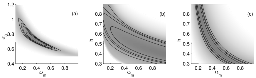
Figure 1: (a) The cluster abundance likelihood function in the {$\Omega_{\rm{m}}$,$\sigma_{8}$}-plane, after marginalisation over $h$. (b) The CMB likelihood function in the {$\Omega_{\rm{m}}$, $h$}-plane, after marginalisation over $\sigma_{8}$. (c) The IRAS likelihood function in the {$\Omega_{\rm{m}}$, $h$}-plane, after marginalisation over $\sigma_{8}$ and $b_{\rm IRAS}$. The contours denote the 68, 90, 95 and 99 per cent confidence regions.

2 Individual data sets

2.1 Cluster Abundances

A range of different values for cosmological parameters have been inferred from the evolution of the number density of clusters with redshift (e.g. Frenk et al. 1990; Carlberg et al. 1997; Bahcall, Fan & Cen 1997; Blanchard & Bartlett 1998; Reichart et al. 1999), and in some cases the quoted uncertainties are sufficiently small to make the results incompatible. This implies that systematic uncertainties are important (see Eke et al. 1998 for a discussion). For a joint likelihood analysis, the resulting confidence limits on the inferred cosmological parameters are only reliable if the systematic errors present in the individual analyses are less important than the statistical ones. For this reason, the cluster abundance is addressed using the X-ray temperature function, where this is least unlikely to be the case.

We use two X-ray flux-limited samples. The first is comprised of the 25 clusters with average redshift 0.05 compiled by Henry & Arnaud (1991). We have incorporated the latest temperature measurements from Ginga and ASCA for these clusters (Henry 1999). The second sample is comprised of 14 Einstein Extended Medium Sensitivity Survey (EMSS) clusters with average redshift 0.38 compiled by Henry (1999). The temperatures of all 14 clusters have been determined with ASCA data using the most recent calibrations available (Henry 1999). In order to calculate likelihoods the Press-Schechter (1974) expression for the abundance of rich clusters as a function of mass and redshift, coupled with a mass-temperature conversion (White et al. 1993; Eke et al. 1998) is employed to predict the distribution of cluster redshifts and temperatures for each model. These are compared with the observed distributions as discussed by Henry (1997) and Eke et al. (1998), using the ‘default’ assumptions detailed by Eke et al. (1998).

As discussed in Section 1, the main constraint from cluster abundances is in the $\sigma_{8}$, $\Omega_{\rm{m}}$ plane, and this is plotted in Fig. 1 (a).

2.2 CMB

Our approach follows that of Hancock et al. (1998) and Webster et al. (1998). We use the same data as Webster et al., with the addition of the recent QMAP points (de Oliveira-Costa et al. 1998). This same data set is used and plotted in Efstathiou et al. (1998).

The flat band-power method is employed (as described in e.g. Hancock et al. 1998), although Bartlett et al. (1999) and Bond, Jaffe & Knox (1998) find that this approximation widens the error ranges on the cosmological parameters. The conclusions of this letter would not be significantly affected by such a change.

We assume that there are negligible tensor contributions to the CMB power spectrum, as predicted by most inflation models. We also assume neglible re-ionisation and a Harrison-Zel’dovich primordial power spectrum (ie. the primordial spectral index $n=1$) as favoured by inflation and the CMB data. We note that changing these assumptions would substantially alter our results. The remaining family of Cold Dark Matter models are analysed using the Boltzmann code of Seljak & Zaldarriaga (1996).

The CMB COBE data point constrains the large scale temperature fluctuations well. This converts to a strong constraint on $\sigma_{8}$ for each $h$ and $\Omega_{\rm{m}}$. Estimates of the location and height of the first acoustic peak are also provided by the CMB data, and these constrain a degenerate combination of $h$ and $\Omega_{\rm{m}}$ (Fig. 1 (b)). Putting these together also places a weak constraint on $\sigma_{8}$.

2.3 IRAS 1.2 Jy survey

The data and method used here are exactly as in Fisher et al. (1994) and Webster et al. (1998). We use a sample of 5313 IRAS galaxies flux-limited to 1.2 Jy at 60 $\mu$m, selected from the IRAS data base (Strauss et al. 1990, Fisher 1992), and calculate redshift weighted spherical harmonics which may be compared with those predicted given a matter power spectrum. We use Gaussian windows for the redshift weighting, and take into account the redshift distortion using an approximation that is correct only in linear theory. Therefore in this analysis we use only spherical harmonics up to $l=10$ so that the scales probed are large, and the fluctuations can be assumed to be in the linear regime.

It is assumed that the relationship between the galaxy distribution and the matter distribution can be described by the single parameter, the biasing factor for the IRAS galaxies, $b_{\rm IRAS}$. In practice the relationship between the two power spectra may have many dependencies, including scale dependence. Note that if $b_{\rm IRAS}$ is actually scale dependent then the information on the shape of the power spectrum given by the IRAS data would be wrong. However, if the assumption of scale independent biasing is correct then galaxy survey data such as the IRAS 1.2 Jy survey place powerful constraints on the shape of the power spectrum in the scale range examined. The redshift distortion also provides limits on $\beta_{\rm IRAS}=\Omega_{\rm{m}}^{0.6}/b_{\rm{IRAS}}$ and hence a constraint on $\Omega_{\rm{m}}$ for each value of $b_{\rm{IRAS}}$. However, this turns out to be a relatively weak constraint. Nevertheless, the range of values of $\Omega_{\rm{m}}$ allowed by IRAS together with CMB or cluster abundances lies well within the range allowed by IRAS alone. Thus, for this paper, the most important constraint from the IRAS data is that on the shape of the matter power spectrum which, as will be seen in the next section, manifests itself in the $\Omega_{\rm{m}}$, $h$ plane, plotted in Fig. 1 (c).

3 Combining the data sets

3.1 Parameters

In this letter the three cosmological parameters we vary are: the present day value of the reduced Hubble constant, $h=H_{0}/(100$ $\rm{km}\rm{s}^{-1}\rm{Mpc}^{-1}$$)$, the matter density of the universe in units of the critical density, $\Omega_{\rm{m}}$, and the matter power spectrum normalisation parameter, $\sigma_{8}$, the rms linear fluctuation of matter density in $8h^{-1}$ Mpc spheres. The fourth parameter is $b_{\rm IRAS}$, which should be regarded as a ‘fudge factor’ reflecting our ignorance on how to relate fluctuations in galaxy counts to fluctuations in mass. We assume that the universe is flat so that $\Omega_{\rm{m}}+\Omega_{\Lambda}=1$ as suggested by recent analyses of CMB data which allow for $\Omega_{\rm{m}}$ and $\Omega_{\Lambda}$ to vary independently (eg. Lineweaver 1998; Tegmark 1998; Efstathiou et al. 1998).

To transform the information on the shape of the matter power spectrum provided by the IRAS and cluster abundance data into constraints in the parameter space we consider, we use the Bardeen et al. (1986) approximation formula for the matter power spectrum, parameterised by the shape parameter, $\Gamma$. We use the approximate expression provided by Sugiyama (1995),

$$\Gamma=\Omega_{\rm{m}}\,h\ {\rm exp}\left({-\Omega_{\rm{b}}\left[1+{{\sqrt{h/0.5}}\over{\Omega_{\rm{m}}}}\right]}\right)\ .$$ (1)

This, and the CMB power spectrum calculation, require a value for the baryon density which we take from the nucleosynthesis constraint, $\Omega_{\rm{b}}h^{2}=0.019$ (Burles & Tytler 1998). Our results are relatively insensitive to this value.

Using this conservative number of parameters allows a more thorough examination of the parameter space, and despite our large number of assumptions, we find remarkable agreement between the data sets.

3.2 Statistical issues

Comparing results from different data sets enables us to shed some light on how well our current picture of cosmology stands up. This kind of comparison could be performed by simply comparing the parameter values predicted by different data . While this is a start, it does not take into account the fact that most measurements are sensitive to more than one parameter. A full examination of the level of agreement between data sets should include a comparison of likelihood values in multi-dimensional space. In this letter we have considered the four free parameters $\Omega_{\rm{m}}$, $\sigma_{8}$, $h$ and $b_{\rm IRAS}$ and found that there is a region in the four-dimensional space in which the likelihood functions of each data set are high. This is important to check before simply multiplying likelihoods, because the final best fit point could be a bad fit to all the data sets used, even if the one-dimensional marginalised joint likelihood functions for each parameter look promising. The goodness of fit of each data set can be evaluated e.g. by $\chi^{2}$.

Combining results is also powerful because the parameter degeneracies from each data set may be complementary. Fig. 2 shows a three-dimensional view of the orthogonality of the CMB and cluster abundance confidence surfaces. The favoured region of parameter space is very much smaller than the regions of parameter space allowed by the single data sets alone, thus yielding much tighter constraints. This joint likelihood function is computed by calculating likelihoods over a grid in parameter space, then multiplying them together for the different data sets.

Note that multiplication of the likelihoods for each data set is strictly correct only in the case where the data sets are independent. While the CMB clearly probes a different part of the universe to either the IRAS galaxies or the cluster abundance clusters, it is not so clear whether there is some overlap in the IRAS and low redshift cluster data. In this letter we assume that these two data sets are independent, and justify it on the basis that (a) the redshift ranges do not overlap significantly, the low redshift clusters having a median redshift of 0.05, while the IRAS galaxies have a median redshift of 0.02 and (b) because IRAS galaxies are selected in the infra-red, they tend to be field galaxies and so are not likely to be in the clusters sampled in the cluster survey. This issue also affects the CMB analysis, since the flat band power $\chi^{2}$ analysis is not valid if the observations used overlap on the sky and in angular scale range (spherical harmonic $\ell$ range). We have avoided this by using a set of CMB data points that do not overlap in this way, but the set of data points chosen could be argued to be somewhat subjective.

We obtain confidence limits on each cosmological parameter by marginalising over the other parameters. If the parameters are well enough constrained then the integration limits used for the marginalisation will not affect the results. The Bayesian interpretation of the integration limits is that we have ‘top hat’ priors on each parameter. For the integration in the marginalisation we use $0.2<\sigma_{8}<1.4$, $0.3<h<0.9$, $0.1<\Omega_{\rm{m}}<1.0$ and $0.7<b_{\rm IRAS}<2.0$ (in 100, 100, 100, 50 steps respectively). The parameters are so poorly constrained by any single data set that these integration limits do affect some marginalised results. For example, our range of integration in $\sigma_{8}$ affects the two-dimensional plot of $h$ and $\Omega_{\rm{m}}$ for the CMB data (Fig. 1 (b)), making the contours foreshorten at low $\Omega_{\rm{m}}$. However, we choose our limits to be wide enough that they do not affect the results when using more than one data set at a time. Thus the one-dimensional marginalised distributions for pairs of data sets plotted in Fig. 3 (a) are independent of the priors. This integration process is computationally costly, and some authors utilise approximations at this point. For example Lineweaver (1998) and Tegmark (1998) ‘project’ the likelihood function to one dimension, taking the maximum value of the likelihood found on varying the other parameters, rather than integrating over all the values of the likelihood for all the possible values of the other parameters. This approximation is correct when the likelihood function is a Gaussian, but not otherwise. Note that when we talk about the 68 per cent confidence surface or contour we mean the (iso-probability) boundary to the region containing 68 per cent of the probability (given our top hat priors).

4 Results

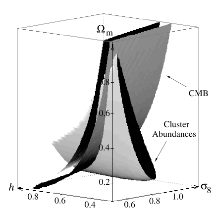
Figure 2: CMB and cluster abundance iso-probability surfaces plotted in three-dimensions, for $\Delta$log(Likelihood)=7.1 (3$\sigma$ for a 3d Gaussian probability distribution).

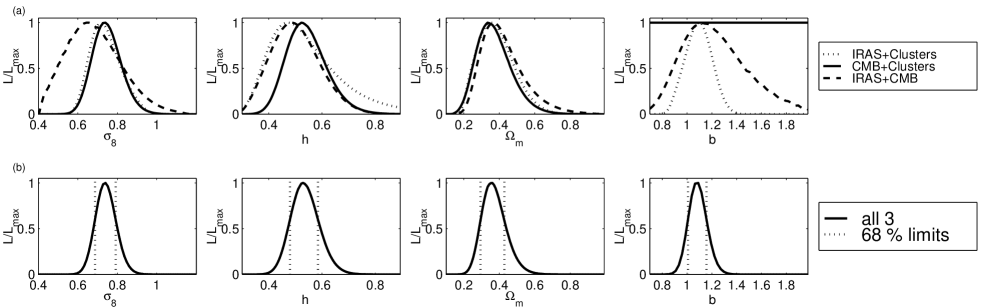
Figure 3: The 1d marginalised distributions using (a) pairs of data sets and (b) using all three data sets. The dotted lines denote 68 per cent confidence limits.

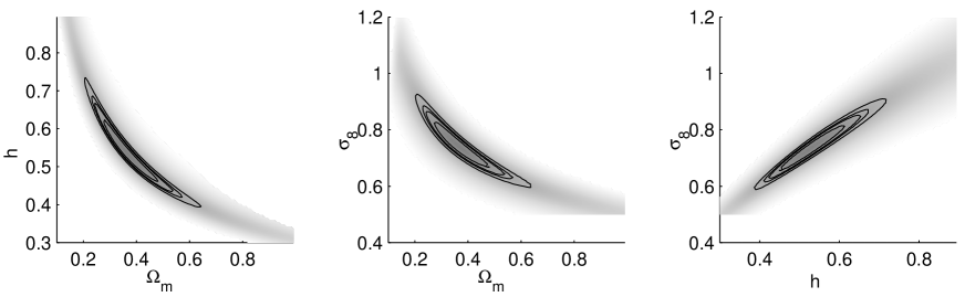
Figure 4: The likelihood function from combining all three data sets as a function of pairs of parameters, in each case marginalised over the remaining two parameters. The contours denote the 68, 90, 95 and 99 per cent confidence regions.

Since it is possible to choose reasonable integration ranges such that the results using any pair of data sets are independent of the integration ranges, we may say that just a pair of data sets is sufficient to constrain properly these four parameters (or three parameters for CMB and cluster abundances).

The results for pairs of data sets are shown in Fig. 3. It can be seen that these three data sets are in extremely good agreement, since the parameter values preferred by each pair are consistent. This is particularly apparent for $\Omega_{\rm{m}}$. It is a result of the fact that all three 68 per cent confidence surfaces intersect in the same place in three and four dimensions. It was therefore not surprising to find that the best fit point given in Table 1 is within the 68 per cent confidence surface for each single data set.

Parameter Best fit point 68 per cent confidence limits $\Omega_{\rm{m}}$ $0.36$ $0.30\,<\,\Omega_{\rm{m}}\,<\,0.43$ $h$ $0.54$ $0.48\,<\,h\,<\,0.59$ $\sigma_{8}$ $0.74$ $0.69\,<\,\sigma_{8}\,<\,0.79$ $b_{\rm IRAS}$ $1.08$ $1.01\,<\,b_{\rm IRAS}\,<\,1.16$

Table 1: Parameter values at the joint optimum. The 68% confidence limits are shown, calculated for each parameter by marginalising the likelihood over the other variables.

For the parameter values at the best fit point, the shape parameter for the mass power spectrum $\Gamma=0.15\pm 0.02$, the baryonic density $\Omega_{\rm{b}}=0.066\pm 0.013$, the CMB quadrupole $Q_{\rm{rms-ps}}=18.0\pm 1.0\mu$K, the IRAS distortion parameter $\beta_{\rm{IRAS}}\equiv\Omega_{\rm{m}}^{0.6}/b_{\rm IRAS}=0.50\pm 0.05$ and the age of the universe is $16.7\pm 1.0$ Gyr. In each case, the errors correspond to the estimated 68 per cent marginalised confidence limits.

As an indicator of how well the joint optimum fits each data set alone we calculate the $\chi^{2}$ value at the joint optimum for each of the CMB and IRAS data sets, using the method described in Webster et al. (1998). The CMB $\chi^{2}$ is 22.8 (we use 23 CMB data points) and the IRAS $\chi^{2}$ is $142$ (for spherical harmonics up to $l=10$ there are $120$ degrees of freedom), suggesting that the predicted observations agree well with the actual observations for the parameters at the joint optimum. Because of the unbinned nature of the cluster abundance analysis, it is more complicated to find a similar statistic. However, as discussed by Eke et al. (1998), all of the models considered predict a relatively even distribution of clusters over the range $0.3<z<0.4$, but in actual fact there are many more clusters at the low end of this redshift range than predicted by any of the models considered. This suggests that the selection function for the clusters was poorly modelled, inevitably leading to a poor goodness of fit to the cluster data, independent of the parameter values used in the model (given the assumptions of this paper). The number of clusters predicted from the best fitting model is $19.5$ at low redshift and $26$ at high redshift. This may be compared to the actual numbers observed, $25$ and $14$ respectively, and can be seen to differ by more than the 1$\sigma$ of $\sqrt{N}$ expected from Poisson statistics.

The 1d and 2d marginalised distributions given all three data sets are also shown in Figs. 3 and 4. It can be seen that adding in a third data set tightens the constraints further and the 68 per cent confidence limits obtained from these 1d distributions are presented in Table 1.

5 Discussion

The non-trivial and reassuring result is that the marginalised distributions of the parameters are consistent when single data sets, or any combination of two data sets, are included. This means that no single experiment is dominating or pushing the favoured parameter values away from the otherwise preferred ones. It is thus tempting to suggest that systematic uncertainties in the individual data sets may not be greatly affecting the parameter values that have been inferred by this analysis.

The strong agreement between pairs of data sets can be understood qualitatively as follows. The cluster abundance data provide a strong constraint on $\sigma_{8}$; the CMB provides a much weaker limit on $\sigma_{8}$ but one which agrees with the cluster abundance limit. The IRAS data provides limits on the combination $\sigma_{8}b_{IRAS}$ and so putting this together with the above constraint on $\sigma_{8}$ produces a small allowed range of $b_{\rm IRAS}$. The cluster abundance data also favour just a small range in $\Omega_{\rm{m}}$. The different degeneracy directions in the $\Omega_{\rm{m}}$,$h$ plane from each of the CMB and IRAS data produce a slightly weaker limit on $\Omega_{\rm{m}}$, but one which agrees with the cluster abundance result. Putting together the strong cluster abundance constraint on $\Omega_{\rm{m}}$ with either the CMB or IRAS limits in the $h$, $\Omega_{\rm{m}}$ plane produces a constraint on $h$; alternatively, just the CMB and IRAS data can be used to determine an allowed range in $h$; and each of these routes to $h$ produces the same answer.

Our results agree well with other recent work which combines data sets to set limits on cosmological parameters (Bond & Jaffe 1998, Gawiser & Silk 1998, Lineweaver 1998, White 1998, Garnavich et al. 1998, Eisenstein et al. 1998 and Roos & Harun-or-Rashid 1999).

The recent Type 1a supernova results of Perlmutter et al. (1998) imply that for a flat universe $\Omega_{\rm{m}}=0.28^{+0.09}_{-0.08}$ (1$\sigma$ statistical errors), in good agreement with the values derived in this letter. Similar results are also found by Riess et al. (1998). From gravitational lensing measurements, Falco, Kochanek & Munoz (1998) find that $\Omega_{\rm{m}}>0.38$ at 2 sigma, although Chiba and Yoshi (1999) find that a flat universe with $\Omega_{\rm{m}}=0.3^{+0.2}_{-0.1}$ is preferred. Our value for the Hubble constant, $h=0.54$, falls at the low end of the latest distance ladder measurements (Freedman et al. 1998). The optimal baryon density (given $\Omega_{\rm{b}}h^{2}=0.019$) is $\Omega_{\rm{b}}=0.066$, and dividing by our best fit value of $\Omega_{\rm{m}}=0.36$ our optimal baryon fraction is $0.18$ This may be compared to cluster baryon fraction estimates, for example, White et al. (1993) find $\Omega_{\rm{b}}/\Omega_{\rm{m}}\geqslant 0.015+0.08h^{-3/2}$. Inserting our best fit value for $h$ yields $\Omega_{\rm{b}}/\Omega_{\rm{m}}\geqslant 0.22$. Our value for the combination $\sigma_{8}\Omega_{\rm{m}}^{0.6}=0.40$ is lower than the one derived from measurements from the peculiar velocity field $\sigma_{8}\Omega_{\rm{m}}^{0.6}\approx 0.8$ (Freudling et al. 1998). It is closer to the value recently derived from cluster peculiar velocities by Watkins (1997) of $\sigma_{8}\Omega_{\rm{m}}^{0.6}=0.44^{+0.19}_{-0.13}$. Reassuringly, the age of the universe we find ($16.7$ Gyr) is greater than the age of the oldest stars (Chaboyer et al. 1998).

ACKNOWLEDGMENTS

We would like to thank Graça Rocha for her work on compilation of the CMB data set. SLB, VRE, SC and CSF acknowledge the PPARC for support in the form of a research studentship, postdoctoral, advanced and senior fellowships respectively. JPH acknowledges NASA grants NAG5-2523 and NAG5-4828.

References

- [1] Bahcall, N. A., & Cen, R., 1993, ApJ, 407, L49
- [2] Bahcall, N. A., Fan, X., & Cen, R. 1997, ApJ, 485, L53
- [3] Bardeen, J. M., Bond, J. R., Kaiser, N., & Szalay, A.,S. 1986, ApJ, 304, 15
- [4] Bartlett, J., Blanchard, A., Douspis, M., & Le Dour, M. 1998 To be published in “Evolution of Large-scale Structure: from Recombination to Garching”, proceedings of the MPA/ESO workshop, August, 1998 (astro-ph/9810318)
- [5] Bartlett, J., Douspis, M., Blanchard, A., & Le Dour, M. 1999, preprint (astro-ph/9903045)
- [6] Blanchard, A., & Bartlett, J. G. 1998, A&A, 332, L49
- [7] Bond, J. R. & Jaffe, A. H., 1998 Philosophical Transactions of the Royal Society of London A, 1998. “Discussion Meeting on Large Scale Structure in the Universe,” Royal Society, London, March 1998.
- [8] Bond, J. R., Jaffe, A. H., & Knox, L. E. 1998, preprint (astro-ph/9808264)
- [9] Branchini, E., et al., 1999, MNRAS, in press (astro-ph/9901366)
- [10] Burles, S., & Tytler, D. 1998, preprint (astro-ph/9803071)
- [11] Carlberg, R. G., Morris, S. L., Yee, H. K. C., & Ellingson, E. 1997, ApJ, 479, L19
- [12] Chaboyer, B., Demarque, P., Kernan, P. J., & Krauss, L. M. 1998, ApJ, 494, 96
- [13] Chiba, M., & Yoshii, Y. 1999, ApJ, 510, 42
- [14] de Oliveira-Costa, A., Devlin, M., Herbig, T., Miller, A., Netterfield, B., Page, L., & Tegmark, M. 1998, ApJ, 509, L77
- [15] Edge, A. C., Stewart, G. C., Fabian, A. C., Arnaud, K. A., 1990, MNRAS, 258, L1
- [16] Efstathiou G., Bridle S. L., Lasenby A. N., Hobson M. P., Ellis R. S. 1998, MNRAS, accepted (astro-ph/9812226)
- [17] Eisenstein, D. J., Hu, W., & Tegmark, M. 1998, preprint (astro-ph/9807130)
- [18] Eke V. R., Cole S., Frenk C. S., 1996, MNRAS, 282, 263
- [19] Eke, V. R., Cole, S., Frenk, C. S., & Henry, J. P. 1998, MNRAS, 298, 1145
- [20] Falco, E. E., Kochanek, C. S., & Munoz, J. A. 1998, ApJ, 494, 47
- [21] Fisher, K. B. 1992, PhD thesis, Univ. California, Berkeley
- [22] Fisher, K. B., Scharf, C. A., & Lahav, O. 1994, MNRAS, 266, 219
- [23] Freedman, W. L., Mould, J. R., Kennicutt, R. C., & Madore, B. F. 1998, preprint (astro-ph/9801080)
- [24] Frenk, C. S., White, S. D. M., Efstathiou, G., Davis, M., 1990, ApJ, 351, 10
- [Freudling et al. 1998] Freudling, et al. 1998, ApJ, submitted
- [25] Garnavich, P. M. et al. 1998, ApJ, 509, 74
- [26] Gawiser, E., & Silk, J. 1998, Science, 280, 1405
- [27] Hanami, H. 1993, ApJ, 415, 42
- [28] Hancock, S., Rocha, G., Lasenby, A. N., & Gutierrez, C. M. 1998, MNRAS, 294, L1
- [29] Henry, J. P. 1997, ApJ, 489, L1
- [30] Henry, J. P. 1999 in preparation.
- [31] Henry, J. P., & Arnaud, K. A. 1991, ApJ, 372, 410
- [32] Lilje, P. B. 1992 ApJ, 386, L33
- [33] Lineweaver, C. H. 1998, ApJ, 505, L69
- [34] Oukbir, J. & Blanchard, A. 1992, A&A, 262, L21
- [35] Perlmutter, S., et al. 1998, ApJ, accepted (astro-ph/9812133)
- [36] Press, W. H., Schechter, P., 1974, ApJ, 187, 425
- [37] Reichart, D. E., Nichol, R. C., Castander, F. J., Burke, D. J., Romer, A. K., Holden, B. P., Collins, C. A., Ulmer, M. P., 1999, ApJ, accepted (astro-ph/9802153)
- [38] Riess, A. G., et al. 1998, AJ, 116, 1009
- [39] Roos, M., & Harun-or-Rashid, S. M. 1999, preprint (astro-ph/9901234)
- [40] Seljak, U., & Zaldarriaga, M. 1996, ApJ, 469, 437
- [41] Strauss, M. A., Davis, M., Yahil, A. & Huchra, J. P. 1990, ApJ, 361, 49
- [42] Sugiyama, N. 1995, ApJS, 100, 281
- [43] Sutherland, W., et al. 1999, MNRAS, accepted (astro-ph/9901189)
- [44] Tadros, H., et al. 1999, MNRAS, accepted (astro-ph/9901351)
- [45] Tegmark, M. 1998, preprint (astro-ph/9809201)
- [46] Viana, P. T. P., & Liddle, A. R. 1996, MNRAS, 281, 323
- [47] Viana, P. T. P., & Liddle, A. R., 1999, MNRAS, accepted (astro-ph/9803244)
- [48] Watkins, R. 1997, MNRAS, 292, L59
- [49] Webster, A. M., Bridle, S. L., Hobson, M. P., Lasenby, A. N., Lahav, O., Rocha, G. 1998, ApJ, 509, L65
- [50] White, M. 1998, ApJ, 506, 495
- [51] White, S. D. M., Efstathiou, G., & Frenk, C. S. 1993, MNRAS, 262, 1023
- [52] White, S. D. M., Navarro, J. F., Evrard, A. E., & Frenk, C. S. 1993, Nature, 366, 429