A conspicuous increase of Galactic contamination over CMBR anisotropies at large angular scales

Abstract

New calculations of the Galactic contamination over microwave background radiation anisotropies are carried out. On one hand, when a frequency-dependent contrast of molecular clouds with respect to the Galactic background of the diffuse interstellar medium is taken into account, the anisotropic amplitude produced by Galactic dust is increased with respect to previous calculations and this is of the same order as that of the data from the observations. On the other hand, if we take into account rotational dust emission, for instance, a frequency independence of anisotropies in the microwave range may be obtained.

This leads to the possibility that under some particular, but not impossible, conditions all the microwave background radiation anisotropies may be due to Galactic foregrounds rather than cosmological in origin. Moreover, a suspected coincidence between the typical angular sizes of the microwave background radiation anisotropies and those of nearby molecular clouds makes more plausible the hypothesis of a purely Galactic origin for these anisotropies. It is also argued that the correlation among structures at different frequencies, the comparison of the power spectrum at different frequencies and the galactic latitude dependence of the anisotropies are not yet proofs in favour of either a cosmological or Galactic origin.

1 Introduction

Various observations of the cosmic microwave background radiation (CMBR) have led to the claim that it is anisotropic (see reviews Readhead & Lawrence 1992; White, Scott & Silk 1994). Measurement of these anisotropies provides information on structural formation, inflation, quantum gravity, topological defects (strings, etc.), dark matter type and abundance, the determination of $H_{0}$, $\Omega$, $\Lambda$, the geometry and dynamics of the Universe, the thermal history of the Universe at the recombination epoch, etc. A knowledge of these anisotropies is very important for discriminating among different cosmological models as well as for measuring certain related parameters.

Unfortunately, this information is contaminated by several effects which are unrelated to cosmology, and which are either extragalactic or Galactic in origin. Extragalactic sources of such contamination may be gravitational scattering due to inhomogeneities in the matter distribution of superclusters (Fukushige, Makino & Ebisuzaki 1994; Suginohara, Suginohara & Spergel 1998), inhomogeneous reionization (Knox, Scoccimarro & Dodelson 1998), possible radiative decay of massive tau neutrinos (Celebonovic, Samurovic & Circovic 1997), the inverse Compton effect, temporal variations of the gravitational potential, etc. This paper will not analyse such extragalactic sources of anisotropy but will concentrate instead on those coming from our own Galaxy, particularly at large angular separations ($\theta>2^{\circ}$).

A summary of possible contributions from our own Galaxy to the anisotropies has been studied, for instance, by Bennett et al. (1992) and has led to the conclusion that there are three possible emission mechanisms: synchrotron, free-free and dust emission. The calculation of anisotropies originating in our Galaxy was carried out on the basis of observations from the COBE-DIRBE, which were extrapolated to other frequencies, and it was concluded that Galactic contamination is negligible. The paper of Bennett et al. was optimistic. However, not all authors think the same. Masi et al. (1990) pointed out that dust may provide an important contribution to the anisotropies in the microwave region. Banday & Wolfendale (1991) predicted that dust contamination is quite important except in some regions away from the cirrus. Hence, whether or not the dust contribution is negligible seemed to be a point of contention by the beginning of nineties.

Recently, clear evidence of correlations between far-infrared maps (which trace Galactic dust) and microwaves has been presented (Kogut et al. 1996a, de Oliveira-Costa et al. 1997; de Oliveira-Costa et al. 1998). In the light of these works it is difficult to deny the influence of the Galaxy on the microwave background. Even though the source of the contamination remains unknown, the correlation between the Galaxy and COBE-DMR data remains an observational fact. Another recent paper written by Pando, Valls-Gabaud & Fang (1998) points out the non-Gaussian nature of the CMBR over large angular scales of anisotropies against standard cosmological predicitions, and this might be due to an excess of foreground contamination.

In this paper, an explanation is offered for these last observational facts. Two new elements are added to previous works for the calculation of Galactic contamination: a frequency-dependent contrast of molecular clouds with respect to the Galactic background of the diffuse interstellar medium; and the existence of a recently noticed source of emission: rotational emission by dust grains (Draine & Lazarian 1998a). These lead to a non-negligible and possibly unique source of anisotropies due to our Galaxy.

2 How large is the Galactic contamination?

The existence of flux anisotropies due to Galactic clouds is undeniable. In the far infrared, the presence of the molecular clouds is associated with “infrared cirrus”. There is a good correlation between infrared cirrus and atomic hydrogen gas (Boulanger, Baud & van Albada 1985; Burton & Deul 1987; Boulanger & Pérault 1988; Schlegel, Finkbeiner & Davis 1998) and the fluctuations of the hydrogen column densities within the nearest 75 to 100 pc of the Sun are occasionally about $5\times 10^{19}$ cm^-2 (Frisch & York 1986), so this implies that fluctuations due to nearby clouds must be detected to some extent in the microwave region.

Most of the clouds are confined in the Galactic plane but there are few which can be observed at high galactic latitudes, and which are close to us (Blitz 1991). Those responsible for large angle correlations would need to have a large size (i.e. giant molecular clouds). So, some microwave background radiation anisotropies (MBRAs) may be due to inhomogeneities in the density distribution of the local interstellar medium.

Dust associated with these giant clouds exists in three different stages associated with molecular, neutral and ionized hydrogen (Sodroski et al. 1997), whose total emission gives a continuum spectrum proportional to the column density in the line of sight. Column density fluctuations lead to intensity fluctuations. Dust anisotropies would be due to its non-homogeneous distribution in molecular clouds or its equivalent for other types of Galactic emission.

Dark matter around spiral galaxies in the form of cold gas, essentially in molecular form and rotationally supported, was purposed by Pfenninger, Combes & Martinet (1994) and Pfeninger & Combes (1994); this cold gas in molecular form was also held to contribute at microwave wavelengths (Schaefer 1994; Schaefer 1996). The gas would be at temperatures close to $3$ K and composed of small clumpuscules of size $30$ AU. It is claimed (Combes & Pfenniger 1997; Schaefer 1996) that part of the radiation observed by COBE-FIRAS is cold gas instead of dust. It might be in the outer disc and difficult, although not impossible, to detect. Indeed, Combes & Pfenninger (1997) propose techniques for detecting it. Though this cold gas may be a source of anisotropies, it would be only for very small scales since the emission is high enough just for very high densities ($n(H_{2})\sim 10^{18}$ cm^-3) inside the small clumpuscules. Thence, cold molecular gas emission will not be further considered.

In following subsections, the expected emission from our Galaxy will be compared with observations in the microwave region.

2.1 MBRAs amplitude

The two-point correlation function is:

$$\langle T^{*}T^{*}\rangle(\theta)=\int d\Omega\int_{|\Omega^{\prime}-\Omega|=\theta}d\Omega^{\prime}T^{*}(\Omega)T^{*}(\Omega^{\prime})$$ (1)

, where $T^{*}$ is the antenna temperature, once the average flux is subtracted, the results are those shown in Fig. 2 and 3.

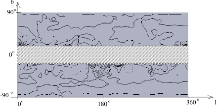
Figure 1: The COBE-DIRBE flux map at 240 $\mu$m after subtraction of a smooth component of the Galactic background as explained in the text. The contours are from –20 to +20 MJy sr^-1 in steps of 4 MJy sr^-1.

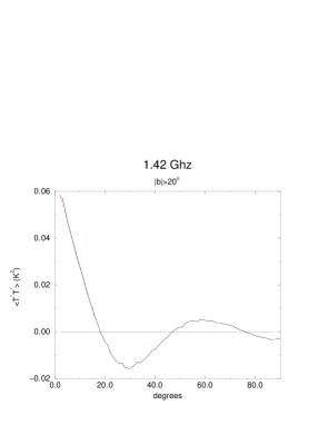
a)

Figure 2: Angular correlation function for different surveys at $|b|>20^{\circ}$: a) 1.42 GHz (the Max Planck Institute for Radio Astronomy, Reich 1982; Reich & Reich 1986), the dashed line is a fit to $0.0663-0.00382\theta({\rm deg.})$ K²; b) 240 $\mu$m (COBE-DIRBE, Boggess et al. 1992), the dashed line is a fit to $2.13\times 10^{-8}\theta({\rm deg.})^{-1.20}$ K².

Fig. 2 b)

Figure 3: Cross correlation function for two surveys: 1.42 GHz (Max Planck Institute for Radio Astronomy, Reich 1982; Reich & Reich 1986) and 240 $\mu$m (COBE-DIRBE, Boggess et al. 1992).

In order to calculate the effects of the Galaxy on MBRAs, extrapolation of the measured two-point correlation functions (Fig. 2) at 1.42 GHz due to synchrotron emission and at 240$\mu$m due to continuum dust emission must be carried out. Free-free emission is not considered here in order to simplify the calculations and because we have no information concerning it (Smoot 1998). In any case, if it is proven than dust or synchrotron emission or both are high enough then adding free-free emission would increase Galactic anisotropies, never decrease.

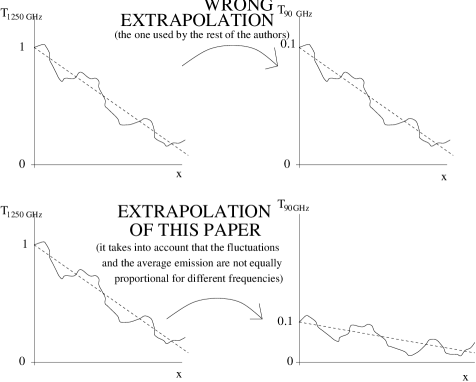
Figure 4: Example of extrapolations for Galactic dust emission. The main difference between the extrapolation of expression (4) and those derived in work prior to this paper is that the latter do not take into account the frequency dependence of the proportionality between the amplitude of the fluctuation and that of the average flux.

At any frequency in the microwave range, two-point correlation functions must be evaluated by extrapolating both effects independently and summing them up according to:

$$\langle T(\nu)T(\nu)\rangle=\langle(T_{\rm synchr}(\nu)+T_{\rm dust}(\nu))$$

$$\times(T_{\rm synchr}(\nu)+T_{\rm dust}(\nu))\rangle=\langle T_{\rm synchr}(\nu)T_{synchr}(\nu)\rangle$$

$$+\langle T_{\rm dust}(\nu)T_{\rm dust}(\nu)\rangle+2\langle T_{\rm synchr}(\nu)T_{\rm dust}(\nu)\rangle.$$ (2)

Each of these terms may be calculated by means of an extrapolation of previously measured correlations. I will calculate the contribution due to the local Galactic flux fluctuations with respect the average flux, i.e. $<T^{*}T^{*}>$, and not that due to the smooth variation of the dependence of this average flux with Galactic coordinates. Usually, the extrapolation is carried out by multiplying each of the pixels of the map at $\nu_{0}$ by the mean amplitude variation of the flux ($\langle T(\nu)/T(\nu_{0})\rangle$) and calculating the correlations of the new map at frequency $\nu$. This is equivalent to multiply the two-point correlation function by a factor $\langle T(\nu)/T(\nu_{0})\rangle^{2}$. I will go one step further and will take into account that the local fluctuations do not vary proportionally to the average flux (Fig. 4); therefore, the mean amplitude of the two-point correlation function is affected by a second factor. As we will see later, this variation is due to different effective dust temperatures between the Galactic clouds which produce the fluctuations and the Galactic medium that contributes to the average flux. The shape of two-point correlation function is also expected to vary, as will be explained in §3.3. However, since we want to estimate only the order of magnitude of the correlation amplitude in the microwave region, we will not take this effect into account at this stage. The effects of the shape variation of the two-point correlation function will be analysed in §3.3.1. Hence, extrapolations are calculated according to

$$\langle T_{{\rm synchr}}(\nu)T_{{\rm synchr}}(\nu)\rangle(\theta)=\left\langle\frac{T_{{\rm synchr}}(\nu)}{T_{{\rm synchr}}(1.42\ {\rm GHz})}\right\rangle^{2}$$

$$\times\left\langle\frac{\left(\frac{\Delta T_{{\rm synchr}}(\nu)}{T_{{\rm synchr}}(\nu)}\right)}{\left(\frac{\Delta T_{{\rm synchr}}(1.42\ {\rm GHz})}{T_{{\rm synchr}}(1.42\ {\rm GHz})}\right)}\right\rangle^{2}$$

$$\times\langle T^{*}_{{\rm synchr}}(1.42\ {\rm GHz})T^{*}_{{\rm synchr}}(1.42\ {\rm GHz})\rangle(\theta),$$ (3)

$$\langle T_{\rm dust}(\nu)T_{\rm dust}(\nu)\rangle(\theta)=\left\langle\frac{T_{\rm dust}(\nu)}{T_{\rm dust}(240\ \mu{\rm m})}\right\rangle^{2}$$

$$\times\left\langle\frac{\left(\frac{\Delta T_{\rm dust}(\nu)}{T_{\rm dust}(\nu)}\right)}{\left(\frac{\Delta T_{\rm dust}(240\ \mu{\rm m})}{T_{\rm dust}(240\ \mu{\rm m})}\right)}\right\rangle^{2}$$

$$\times\langle T^{*}_{\rm dust}(240\ \mu{\rm m})T^{*}_{\rm dust}(240\ \mu{\rm m})\rangle(\theta),$$ (4)

$$\langle T_{{\rm synchr}}(\nu)T_{\rm dust}(\nu)\rangle(\theta)$$

$$=\left\langle\left(\frac{T_{{\rm synchr}}(\nu)}{T_{{\rm synchr}}(1.42\ {\rm GHz})}\frac{T_{\rm dust}(\nu)}{T_{\rm dust}(240\ \mu{\rm m})}\right)\right\rangle$$

$$\times\left\langle\left(\frac{\left(\frac{\Delta T_{{\rm synchr}}(\nu)}{T_{{\rm synchr}}(\nu)}\right)}{\left(\frac{\Delta T_{{\rm synchr}}(1.42\ {\rm GHz})}{T_{{\rm synchr}}(1.42\ {\rm GHz})}\right)}\frac{\left(\frac{\Delta T_{\rm dust}(\nu)}{T_{\rm dust}(\nu)}\right)}{\left(\frac{\Delta T_{\rm dust}(240\ \mu{\rm m})}{T_{\rm dust}(240\ \mu{\rm m})}\right)}\right)\right\rangle$$

$$\times\langle T^{*}_{{\rm synchr}}(1.42\ {\rm GHz})T^{*}_{\rm dust}(240\ \mu{\rm m})\rangle(\theta),$$ (5)

so we have to multiply three factors for any of the correlations: the first factors ($\langle T(\nu)/T(\nu_{0})\rangle$) take into account the variation of the mean Galactic background, the second factors ($\langle\frac{\Delta T}{T}(\nu)/\frac{\Delta T}{T}(\nu_{0})\rangle$) for the variation of relative fluctuations at different frequencies and the third factors ($<T^{*}T^{*}>(\nu_{0},\theta)$) are respectively the correlations measured in Fig. 2 a), 2 b) and 3. The three factors can be separated because of the assumption of the independence of $\theta$ for the first and the second factor.

First factors:

The antenna temperature due to synchrotron emission is

$$T_{{\rm synchr}}(\nu,|b|>20^{\circ})=0.6\left(\frac{\nu}{1420\ {\rm MHz}}\right)^{\beta}\ \ {\rm K},$$ (6)

where $\beta\approx-3$ (Davies, Watson & Gutiérrez 1996). See the contribution in Figure 5.

The dust temperature has two contributions: thermal emission, which is detected at far infrared wavelengths (this is the emission detected at 240 $\mu$m); and the microwave rotational emission due to small spinning grains (Draine & Lazarian 1998a). The first contribution is widely accepted while the second is still usually not included in the calculation of the Galactic contribution to the anisotropies in the microwave range.

The mean thermal dust emission is given (Fig. 5) by Reach et al. (1995):

$$T_{\rm dust}(\nu,|b|>20^{\circ})=\left(\frac{\nu}{900\ {\rm GHz}}\right)^{2}[1.74\times 10^{-5}$$

$$\times B(\nu,T=17.72\ {\rm K})+1.23\times 10^{-4}B(\nu,T=6.75\ {\rm K})]$$

$$\times\frac{c^{2}}{2k\nu^{2}}\ \ {\rm K},$$ (7)

where $B$ is the blackbody radiation intensity, $c$ the light speed, $k$ the Boltzmann constant and $\frac{c^{2}}{2k\nu^{2}}$ is the factor for converting intensities into antenna temperatures. This is an average law for $|b|>20^{\circ}$; as shown by Reach et al. (1995), there may be important deviations from this law for some regions.

The second term of eq. (7) may be due to very cold clouds; their average temperature would be 6.75 K if dust emission were proportional to $\nu^{\alpha}B(\nu,T)$ with $\alpha=2$, although this would be somewhat different if $\alpha$ had another value. Expression (7) is just a fit to the observational COBE-FIRAS data, not a model, and their parameters may not have any direct physical meaning. It was argued by Lagache et al. (1998) that an alternative hypothesis to the existence of these very cold clouds is a Cosmic Far Infrared Background due to distant galaxies of 26 $\mu$K in the range between 400 $\mu$m and 1000 $\mu$m (Puget et al. 1996). Regardless whether or not this hypothesis is true, for our purposes the extragalactic emission can be added to the average flux of the Galaxy. The important thing, as will be seen later, is that the fluctuations of the flux are due to local clouds, and that the average temperature of the sources which are origin of the fluctuations is less than that corresponding to the diffuse emission of the Galaxy (plus any extragalactic background).

The rotational emission is the predicted model by Draine & Lazarian (1998a; preferred model: A), Fig. 5 in this paper, taking into account a hydrogen column density $N(H)=3.9\times 10^{20}[cosec(b)-0.17]$, which includes neutral and ionized hydrogen (Heiles 1976; Reynolds 1991), and averaged over $|b|>20^{\circ}$.

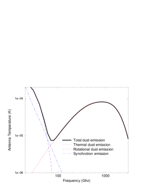
Figure 5: Mean Galactic background emissions for $|b|>20^{\circ}$.

Second factors:

I stress that, as far as I know, all authors who make the extrapolation of correlations set the second factor equal to unity for all frequencies, i.e. the relative fluctuations for dust or synchrotron do not depend on the frequency (for example, Banday & Wolfendale 1991; Bennett et al. 1992; Guarini, Melchiorri & Melchiorri 1995; Reach et al. 1995; Femenía et al. 1998). This is a very poor approximation for dust, especially when the extrapolation is to one order of magnitude for lower frequencies, as it is in this case. I think this poor approximation is the main reason why dust anisotropies were considered negligible in the past.

The reason why I think this is a bad approximation for dust is that the mean dust emission intensity follows a different continuum spectrum from that of the local clouds (infrared cirrus) providing fluctuations at scales of several degrees. When the dust emission is modelled by $I\propto\nu^{\alpha}B(\nu,T)$ (with $B$ the blackbody radiation), $\alpha$ varies from place to place (Tegmark 1998): it is smaller for molecular clouds (Mathis 1990; Schloerb, Snell & Schwartz 1987; Meinhold et al. 1993) or higher latitudes (Banday & Wolfendale 1991; Reach et al. 1995) than that for the mean intensity (Matsumoto et al. 1988; Wright et al. 1991; Reach et al. 1995). Moreover, the mean intensity includes emission from star-forming regions and mass-loss stars in which the dust is hotter than the diffuse or clouds dust (Draine 1994). The $\alpha$ spectral index depends on the grain properties (Wright 1993) varying from 1 to 3.5 (Banday & Wolfendale 1991). It is $\approx 2$ for graphite, $\approx 1.5$ for silicates and $\approx 1$ for layer-lattice materials, such as amorphous carbon (Draine & Lee 1984). The difference is also related to the different distribution of dust-grain sizes in the diffuse interstellar medium and in molecular clouds. The rate of small grains is larger in the diffuse interstellar medium than in the clouds and the temperatures are different implying that the peak emission from clouds occurs at different wavelength as compared with that of the diffuse medium (Greenberg & Li 1996).

These second factors are unknown because the anisotropies are not sufficiently explored for wavelengths longer than 240 $\mu$m. In order to give a rough estimate, a simplifying assumption can be made: the Galactic contribution is the sum of the local clouds—infrared cirrus— ($T_{\rm c}$) plus a diffuse Galactic background ($T_{\rm d}$), where all the anisotropies at angular scales of several degrees are due to anisotropies in the local clouds distribution ($\Delta T_{\rm d}=0$). Hence,

$$T_{\rm dust}=T_{\rm dust,d}+T_{\rm dust,c}$$ (8)

$$\frac{\Delta T_{\rm dust}(\nu)}{T_{\rm dust}(\nu)}=\frac{\left(\frac{\Delta T_{\rm dust,c}(\nu)}{T_{\rm dust,c}(\nu)}\right)}{1+\frac{T_{\rm dust,d}(\nu)}{T_{\rm dust,c}(\nu)}}.$$ (9)

The numerator of this expression is constant for all frequencies because the fluctuations of the temperature due to clouds are proportional to their density fluctuations for any frequency. However, the denominator is not constant. The variations of the rate ${T_{\rm d}}/{T_{\rm c}}$ as a function of the frequency must be estimated to evaluate the second factor.

Dust thermal emission.

For a wavelength of 240 $\mu$m the rate can be directly measured from the COBE-DIBE maps at $|b|>20^{\circ}$, taking $T$ as the total radiation, which includes diffuse and clouds emission; and $T^{*}$ as the radiation once the background is subtracted (as explained above), which is $T^{*}=T_{\rm c}-\langle T_{\rm c}\rangle$. If we assume $\langle|\Delta T_{\rm c}|\rangle\sim\langle T_{\rm c}\rangle$, i.e. the typical fluctuations in the cloud flux is as large as the average of the flux, which is justified in a distribution of few single clouds over $|b|>20^{\circ}$ with many regions having a negligible contribution, then

$$1+\frac{T_{\rm dust,d}(240\mu m)}{T_{\rm dust,c}(240\mu m)}\sim\frac{\int_{|b|>20^{\circ}}d\Omega T(\Omega)}{\int_{|b|>20^{\circ}}d\Omega|T^{*}(\Omega)|}=3.3.$$ (10)

The outcome implies that 30% of the radiation at 240 $\mu$m at $|b|>20^{\circ}$ comes from clouds and 70% from the diffuse interstellar medium. This is just an estimation, but it is not a very bad approach. A comparison could be made with the rate from the model by Cox, Krügel & Mezger (1986) which gives a value even greater: $\sim$ 4.5 in the Galactic disc.

Clouds are colder than the diffuse medium: between 6 and 15 K for molecular clouds and around 16 K for diffuse medium according to Greenberg & Li (1996). Not all the infrared excess can be due to molecular clouds, but all of these are generally colder than the diffuse medium of dust associated with gas. Indeed, infrared-excess clouds are peaks of column density of dust probably associated with molecular gas of colder temperatures than the rest of the dust (Reach, Wall & Odegard 1998, Lagache et al. 1998). Hence, the increase in emission from clouds is 10 or 15 times greater than from the interstellar medium when we compare 240$\mu$m and the microwave region, $\nu<100$ GHz, and it is dominated by clouds emission in the microwave region (see, for example, Fig. 14 of Beichman 1987; or Fig. 1 of Cox, Krügel & Mezger 1986) and

$$1+\frac{T_{\rm dust,d}(\nu<100\ {\rm GHz})}{T_{\rm dust,c}(\nu<100\ {\rm GHz})}\approx 1.$$ (11)

Thus, the second factor for thermal radiation for these microwave frequencies is

$$\left(\frac{\left(\frac{\Delta T_{\rm dust}(\nu<100\ {\rm GHz})}{T_{\rm dust}(\nu<100\ {\rm GHz})}\right)}{\left(\frac{\Delta T_{\rm dust}(240\ \mu{\rm m})}{T_{\rm dust}(240\ \mu{\rm m})}\right)}\right)\sim 3.3.$$ (12)

Dust rotational emission.

A factor must also be taken into account for the rotational emission of the dust. First, an error in the function given by Draine & Lazarian (1998a) may be included in this factor since the paper uses different parameters that are poorly known. Secondly, the rate between small particles and large particles is lower for clouds than for the diffuse interstellar medium (Greenberg & Li 1996) because there are processes that destroy small grains (Puget, Léger & Boulanger 1985; Puget & Léger 1989), and this would decrease the emission. Thirdly, the density in the clouds is also higher, thereby providing higher emission. There is not enough data in the literature to carry out accurate calculations. In any case, my intention is to show the order of magnitude of the Galactic contribution rather than make accurate predictions, so I think it is enough to take the dust rotational emission shape of Fig. 5, divided by $T_{dust}(240{\rm\mu m})$, and multiply this by some free parameter $f$. The range of this parameter will be between 0 and 1, so the intensity of the rotational emission is not overestimated. It will be conservatively estimated in the range of possible values compatible with our knowledge of clouds and rotational emission. The factor has to be less than unity because the values of the anisotropies predicted with a factor 1 exceed the total observational values for anisotropies measured by the COBE-DMR and other surveys.

Summing up, the second factor in the microwave region is taken to be 1 for synchrotron emission, 3.3 for thermal dust emission and an unknown factor $0<f<1$ for rotational emission. The calculation of the second factor corresponding to the total dust emission is calculated for each frequency as a weighted average of the thermal and rotational emissions whose weights are the respective intensities of the first factors.

So, with all this information the question to solve is how large are anisotropies due to the Galaxy at microwave frequencies. The answer is in the eq. (2). For example, at 90 GHz, the results are those shown in Fig. 6. Thermal emission of dust is the predominant one in this range. For this frequency, rotational emission with $f<1$ does not contribute significantly, so the exact value of the factor $f$ may be ignored. Synchrotron effects are also negligible since the relative fluctuations in Fig. 2a) are quite low.

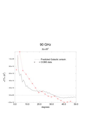
Figure 6: Predicted Galactic two-point correlations at 90 GHz, $|b|>20^{\circ}$, according to eq. (2) compared with the COBE-DMR data (Hinshaw et al. 1996).

As can be observed in Fig. 6, the amplitude of the anisotropy is of the same order as that observed by COBE-DMR. This casts doubts on the origin of MBRAs as, as will be discussed in section 3, they may be totally of Galactic origin.

The results from ULISSE experiment (Bernardis et al. 1992) or other previous experiments (Melchiorri et al. 1981) at 6^∘ scale show that CMBR anisotropies at 90-870 GHz or 410 GHz respectively are less than 35 or 40 $\mu K$ at some regions at high Galactic latitudes, after Galactic emission subtraction. However, these authors use a Galactic emission model which does not take into account the cold molecular clouds discussed in this paper. From eq. (2), averaged over $|b|>20^{\circ}$, $\sqrt{\langle TT\rangle(6^{\circ})(870\ {\rm GHz})}\sim 50\mu K$ (taking the “second factor” as $f\sim 1$ since cold/diffuse clouds flux ratio varies negligibily at these frequencies) and $\sqrt{\langle TT\rangle(6^{\circ})(90\ {\rm GHz})}\sim 19\mu K$ ($f\sim 3.3$). Fluctuations for the intermediate frequencies cannot be calculated since the value of $f$ (second factor) as a function of the frequency is unknown. Nevertheless, it can be seen that the order of magnitude of expected CMBR anisotropies and those from the Galaxy as calculated in this paper are nearly the same.

3 Is it possible that MBRAs are purely Galactic in origin rather than cosmological?

Maybe under some particular, but not impossible, conditions all the microwave background radiation anisotropies be due to Galactic foregrounds rather than cosmological in origin. Some arguments could be given against this and I will discuss them in next subsections.

3.1 Frequency dependence of the MBRAs amplitude

The main argument in favour of a cosmological origin of the MBRAs is that these do not depend on frequency. Strictly speaking, observations point out that the anisotropies at 53 and 90 GHz are nearly the same, but that they are higher at 31 GHz (by a factor 2 or so in difference, Hinshaw et al. 1996). This favours a cosmological origin of the MBRAs but not to the total exclusion of a Galactic origin.

The main argument against Galactic anisotropies with no frequency dependence in the range between 50 and 90 GHz has been that any emission—dust, free-free or synchrotron—-gives a dependence proportional to $\nu^{\alpha}$ with $\alpha\neq 0$. However, we should consider that there may be some range of frequencies of transition between $\alpha>0$—thermal dust emission—and $\alpha<0$—other kinds of emission. The introduction of a quite potent rotational emission (see Fig. 5) is not normally taken into account and it is another important element, which has a negative $\alpha$ for $\nu>20$ GHz. In the intermediate range between both regimes, the amplitude of the anisotropies follows approximately a constant dependence with frequency, i.e. $\alpha\approx 0$.

Is it possible to get from Galactic sources of anisotropies the same two-point correlation function for 53 and 90 GHz as observed by COBE? The answer is yes: when $f\approx 0.8$ (see Fig. 7). As observed in the figure, there is a coincidence in the multiplication of the first and second factors contained in eq. (2) for 53 and 90 GHz, so the amplitude of the correlation will be the same. Synchrotron contribution is low. There is also a dip around 60 GHz which separates slightly from a flat spectrum but this range has not yet been observed accurately. With the present model of rotational emission (model A of Draine & Lazarian 1998a), there is an excess of anisotropies for 31.5 GHz with respect the COBE-DMR observations. This, however, might be reduced when we choose other parameters for the dust rotational emission predictions by Draine & Lazarian (1998a). The aim here has been to show that it is perfectly possible to explain the observational anisotropies at microwave frequencies in terms of Galactic clouds rather than constructing an accurate model. The rotational emission is not well known and there is a lot of work that remains to be done to get exact results. Up to now, only rough estimates can be carried out and these indicate that, contrary to what was believed in the past, there exists the possibility that the totality of the MBRAs are Galactic.

Figure 7: Multiplication of first and second factors of eq. (2) for dust anisotropies when the parameter $f$ is equal to 0.8. Normalized such that $\Delta T(240\mu m)=T(240\mu m)$.

The main objection to this argument might be that it would be an enormous coincidence that $f$ should be 0.8 or, equivalently, in any rotational-emission prediction, that the range of nearly constant $\alpha$ should be between 50 and 90 GHz.

The predicted existence of rotational emission much more intense than free-free emission (Draine & Lazarian 1998a) is controversial and not yet proven. Its existence is used in this paper as a plausible candidate for a non-thermal contribution of emission correlated with dust. However, it is not essential to justify anisotropies at 53 GHz. Other mechanisms could be used instead. Free–free is an option, though there are problems in justifying the necessary flux for the total anisotropies. Another mechanism is the thermal fluctuations of the magnetization within individual interstellar grains when most interstellar Fe exists in a moderately ferromagnetic material (Draine & Lazarian 1998b). This last mechanism might be nearly independent of frequency in the 20-100 GHz range (see Fig. 7 of Draine & Lazarian (1998b) for Fe₃O₄ grains) avoiding the excess at 31.5 GHz described above. At least, one form of contribution—free-free or rotational emission or any other—is necessary to explain the correlations between the anisotropies and far-infrared maps (Kogut et al. 1996a; de Oliveira-Costa et al. 1997; de Oliveira-Costa et al. 1998). The role played by rotational emission with a spectral index $\alpha$ less than zero can be substituted by the free emission or others. It was shown that Galactic cirrus emission is high enough to explain observed anisotropies at 90 GHz (Fig. 6). Whether this level of anisotropy may be maintained for lower frequencies down to 50 GHz would be merely a question of fitting some parameter to other emissions. We can even fit the three or more emission types (free-free, dust rotational, dust thermal emission, magnetic dipole emission from dust grains,…) at the same time in order to get a nearly flat continuum spectrum between 50 and 90 GHz, as well as to get a conspicuous increase for lower frequencies.

3.2 MBRA angular size

One remarkable feature of MBRAs that rouses suspicion about their relationship to our Galaxy is the coincidence of the typical angular size of their structures with the typical angular size of nearby clouds. These structures have an appearance very similar to the clouds observed in other frequencies.

As an example, compare Fig. 4 of Gutiérrez et al. (1997, reproduced in Fig. 8 c)), showing structures observed by the Tenerife Experiment, and Fig. 8 a), b), d), e) for other frequencies. The second differences are evaluated according to

$${\rm Second\ diff.}(\alpha,\delta)=T(\alpha,\delta)-\frac{1}{2}[T(\alpha+8.1^{\circ}/\cos(\delta),\delta)$$

$$+T(\alpha-8.1^{\circ}/\cos(\delta),\delta)],$$ (13)

where $T$ is the antenna temperature of the radiation received in a beam of FWHM=5 deg  .

The aspect of the anisotropies is similar at all frequencies, and the widths of the peaks are similar. However, it is usually claimed that anisotropies between 20 and 100 GHz are predominantly cosmological while the other frequencies are dominated by the Galactic contribution.

a)

Figure 8: Second differences of antenna temperature in different surveys at $\delta=35^{\circ}$: a) 1.42 GHz from the Max Planck Institute for Radio Astronomy (Reich 1982; Reich & Reich 1986); b) 4.85 GHz from NRAO (Condon, Broderick & Seielstad 1991; Condon, Griffith & Wright 1993; Condon et al. 1994); c) 15 GHz from the Tenerife Experiment (Gutiérrez et al. 1997), solid line, and 53 and 90 GHz from COBE-DMR (Bunn, Hoffman & Silk 1996), (Figure taken from Gutiérrez et al. 1997); d) 240 $\mu$m (1250 GHz) from COBE-DIRBE (Boggess et al. 1992); e) 100 $\mu$m (3000 GHz) from IRAS (Wheelock et al. 1994).

Fig. 8 b)

Fig. 8 c)

Fig. 8 d)

Fig. 8 e)

We also see this likeness in Fig. 6. The correlation becomes null—first zero—around 30 deg at both Galactic and observed COBE-DMR. The first zero is related to the average angular size of the clouds when they are responsible for the anisotropies (López-Corredoira et al. 1998), and this coincidence implies that the average angular size of the supposed cosmological structures is approximately equal to that of the nearby clouds giving rise to anisotropies.

The linear size of giant clouds is normally between 20 and 100 pc (Scoville & Sanders 1986) and can even reach sizes between 60 and 300 pc (Magnani, Blitz & Mundi 1985; Heiles, Reach & Boo 1988). The projection of nearby structures such as these gives rise to inhomogeneities and irregular arcs extending between 10^∘ and 50^∘ on the sky (Low & Cutri 1994) in the form of infrared cirrus. In the range from $20$ and $100$ GHz, the Galactic contribution must also provide anisotropies with a first zero around 20 or 30 deg because this is the mean angular size of the clouds, independent of the frequency (the first zero for synchrotron emission is somewhat less than 20 degrees as seen in Fig. 2a). This is precisely what is observed for the total anisotropies. Most authors claim that these anisotropies are cosmological rather than Galactic but the coincidence referred to here might be due to more than just chance. Though this does not prove anything, it is nevertheless a sign in favour of the Galactic predominance in MBRAs.

3.3 Correlation among structures and the power spectrum at different frequencies

Although anisotropies over the whole range of the electromagnetic spectrum may be due to inhomogeneities in the Galactic distribution of dust and gas, this does not mean that the flux maxima and minima at different frequencies must occur at exactly the same coordinates. Several effects—synchrotron, free-free, dust emission, etc.—are responsible for continuum emission but some effects predominate over others at different frequencies. Different effects arise in different regions: synchrotron is higher where magnetic fields are stronger, free-free radiation where a warm ionized medium is present and dust where the coldest temperatures are reached (Bennett et al. 1992). Peaks of dust emission are also to be observed at different positions with different frequencies since cold or warm dust are in different locations; small particles—which are dominant at microwave frequencies (Draine & Lazarian 1998a)—and large particles—which are dominant in the far infrared (Greenberg & Li 1996)—may be distributed differently in the clouds, etc. Thus, we cannot expect uniformity in Galactic structures at different frequencies, i.e. an exact correlation for different frequencies. Such a nonuniformity is observed, for instance, by Davies, Watson & Gutiérrez (1996, their Fig. 10).

In any case, the correlation among different frequencies is not totally null. Comparison of the different plots in Fig. 8 shows a certain correlation. In Fig. 3, some cross-correlation is also observed at scales between 8 and 30 deg, while there is an anticorrelation for less than 8 deg. The microwave continuum in the range between 14 and 90 GHz was also found to be correlated with 100$\mu$m thermal emission from interstellar dust (Kogut et al. 1996a; de Oliveira-Costa et al. 1997; de Oliveira-Costa et al. 1998). This was interpreted as a good correlation existing between dust and free-free emission (Kogut et al. 1996a, 1996b); however, the correlations between H$\alpha$—normally a good tracer of free-free emission—with CMB and DIRBE maps are weak (Leitch et al. 1997; Kogut 1997). Leitch et al. (1997) alternatively proposed an anomalous bremsstrahlung emission from hot gas, but this was again inconsistent with the observed power radiated (Draine & Lazarian 1998a), so other kinds of emissions correlated with dust must be present.

Hence, it must be concluded that correlation among different structures for different frequencies cannot be an argument either for proving or disproving the Galactic origin of the anisotropies, although some non-negligible Galactic contamination is necessary in order to explain these last correlations.

The statistical distribution of the fluctuations given by the two-point correlation function, or its Fourier transform—the power spectrum—is also expected to vary at different frequencies. The coldest parts of the clouds produce dominant emission at lower frequencies so the cloud shapes vary when the frequency varies. Moreover, the dust power spectrum is very sensitive to the region of sky selected (Guarini, Melchiorri & Melchiorri 1995), the background subtraction and other details. As a matter of fact, different spectral indices have been obtained by different authors for the dust emission: $-3.5\leq n\leq-2.5$ (Gautier et al. 1992), $-2.5\leq n\leq-1.5$ (Melchiorri et al. 1996), $n=-2.5$ for $|b|>45^{\circ}$ (Schlegel, Finkbeiner & Davis 1998), etc.

At microwave frequencies, we cannot expect the same power spectra as in the far infrared. Some unknown changes are expected. According to this, power-spectrum or two-point correlation function shapes should not be used to determine whether the anisotropies come from the Galaxy or are cosmological. The fact that the angular power spectra observed at high galactic latitudes by COBE-DIRBE are steeper than the COBE-DMR power spectrum should not be used, as in Wright (1998), to evaluate the degree of Galactic contamination. The shape of the correlation function is also different from the observational data in the microwave region in Fig. 6: there is a deficit of correlation at $\theta\sim 10$ deg and an excess of correlation at $\theta\sim 25$ deg. This may be, as has been said, because the shape of dust in far infrared was extrapolated in spite of the fact that variations were expected (§3.3), and that the cloud intensity fall-off from its centre is different at 240 $\mu$m from that at microwave frequencies.

3.3.1 The magnitude of the effects of the two-point correlation function shape variation with frequency

The extrapolation of dust emission as a combination of three factors was carried out in (4) under the assumption of a non-angular dependence of the first and second factor. This dependence would introduce much more complex calculations for which we do not have accurate enough data (it was not got sufficient information about the correlations at wavelengths longer than 240 $\mu$m), although it can be proven that the order of magnitude of the previous calculations would not change. In any case, the approach taken here is better than any other prior to this paper and the results are more trustworthy.

According to the hypothesis that clouds colder than the diffuse interstellar medium produce the anisotropies, the variation of the temperature within these clouds would produce variations in the $<TT>(\theta)$ shape. In a simple model of emission, in which the cloud flux is proportional to $\nu^{2}B(\nu,T_{t})$, where $T_{t}$ is the effective grain temperature, the antenna temperature $T$ is proportional to $B(\nu,T_{t})$. $T_{t}$ is large enough to take the Rayleigh–Jeans approximation in the microwave range, so $T\propto T_{t}$. This implies that the variation of the antenna temperature in the microwave region is proportional to the variation of the effective grain temperatures. For the calculation of $<TT>(\theta)$, our approach contains a relative error

$$\frac{S(<TT>(\theta))}{<TT>(\theta)}\approx 2\frac{\Delta T_{t}(\theta)}{<T_{t}>},$$ (14)

where $\Delta T_{t}(\theta)$ is the mean variation of $T_{t}$ with respect its average value along two lines of sight separated by an angle $\theta$. This is between $0.7$ and $1.3$ for a maximum relative variation of the effective grain temperature depending of the angle of 15%, which is quite a reasonable value (for instance, clouds within a range of temperatures between 10 and 16 K with a mean temperature of 13 K produce a $T_{t}(\theta)$ between 13 K and 16 K, i.e. 14.5$\pm$ 1.5, a 10%). This may justify the difference of the shape in the plots of Figure 6. In any case, the mean amplitude over the whole range is the one calculated above; there will be some angles in which the amplitude would be higher and others in which it would be lower although the Galactic contamination is within the order of magnitude of the observed anisotropies.

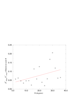
Figure 9: Ratio of flux excesses ($T^{*}$), i.e. after mean background subtraction, between the maps of IRAS 100$\mu$m and DIRBE 240$\mu$ at $|b|>20^{\circ}$ with different filtering scale $\theta$. The solid line is $0.036+0.0021\ \theta$.

From the IRAS 100$\mu$m and DIRBE 240$\mu$m maps, we derive roughly (because the noise is quite high) a dependence between the ratio of flux excesses and the filtering scale $\theta$ (Fig. 9):

$$Ratio=(0.036\pm 0.024)+(0.0021\pm 0.0011)\ \theta$$ (15)

Since this ratio as a function of the filtering scale is equal to $\frac{1}{A}\int f(\theta)\ dA$, where $A=\pi\theta^{2}$ and $f(\theta)$ is the ratio as a function of the correlation angle,

$$f(\theta)=(0.036\pm 0.024)+(0.0031\pm 0.0016)\ \theta.$$ (16)

On the other hand,

$$f(\theta)=\frac{T_{100\ {\rm\mu m}}^{*}}{T_{240\ {\rm\mu m}}^{*}}=\frac{\tau(\nu_{1}^{2}B(\nu_{1},T_{t}(\theta))\frac{c^{2}}{2k\nu_{1}^{2}}}{\tau(\nu_{2}^{2}B(\nu_{2},T_{t}(\theta))\frac{c^{2}}{2k\nu_{2}^{2}}}$$

$$=\frac{\frac{2h\nu_{2}^{3}}{c^{2}}\frac{1}{e^{\frac{h\nu_{1}}{kT_{t}(\theta)}}-1}}{\frac{2h\nu_{1}^{3}}{c^{2}}\frac{1}{e^{\frac{h\nu_{2}}{kT_{t}(\theta)}}-1}},$$ (17)

where $\nu_{1}$ and $\nu_{2}$ are respectively the frequencies corresponding to 100 $\mu$m and 240 $\mu$m. From (16) and (17), we derive a linear dependence (correlation coefficient with a linear fit: 0.9958):

$$T_{t}(\theta)=14.5+0.129\ \theta.$$ (18)

This means that the range of temperatures for angles $\theta$ less than 30 degrees is within $T_{t}=16.4\pm 1.9$ K, i.e. a relative error of 11.5% and the mean temperature of the clouds would be $\langle T_{t}\rangle=14.5$ K (more or less in agreement with the calculations by Lagache et al. 1998). If we use equation (14), this leads to a maximum error of $<TT>(\theta)$ of 23%. This may justify the difference of the shape in the plots of Figure 6, and it does not change the order of magnitude of our calculations. An exact calculation is not carried out since the uncertanties derived from Fig. 9 are too much and the use of a simple model of dust ($\nu^{2}B(\nu,T)$) may be not totally correct to extrapolate $T^{*}$ from the given frequencies to the microwaves (for instance, very small particles may contribute less than a 10% of the total flux (Greenberg & Li 1996) which is negligible for our required accuracy). In any case, this was just to estimate the relative variation with $\theta$ and not to calculate the exact value of $T_{t}$.

3.4 MBRA galactic latitude dependence

From Fig. 10, it is observed that there is some positional dependence of the fluctuations. In this figure, the flux derivative is shown instead of the flux because it allows the fluctuations to be seen more clearly. The variation of the fluctuations at the Galactic poles is something different from that at intermediate latitudes.

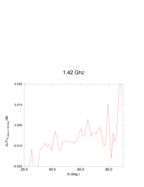
a)

Figure 10: Flux derivative versus Galactic latitude ($b$). a) 1.42 GHz; b) 240 $\mu$m.

Fig. 10 b)

The density distribution of Galactic clouds is irregular with a higher concentration in the plane and a fall-off which can be roughly represented by an exponential with a scale height around 75 pc (Scoville & Sanders 1986). Clouds are distributed very close indeed to the plane. As a matter of fact, nearly all clouds are less than 20 deg from the plane. The remaining clouds that we observe are a few local ones belonging to the plane and are very close to the Sun (Blitz 1991); they are distributed randomly. Any distribution in which the density depends only on $z$, the distance to the plane, should give a column density proportional to $cosec(b)$, but in this case the irregularity makes the density depend also on the other two coordinates, and the column density follows another dependence with respect to $b$. The number of clouds is too small to provide good statistics, so not a lot more can be said about this dependence. Figure 10 may show very slight trends but these are not too clear.

If we do all the calculations of this paper in different regions, for instance: $|b|>30^{\circ}$, $|b|>40^{\circ}$ and $|b|>60^{\circ}$, the correlations expected would be somewhat lower. The anisotropies from dust are shown in Fig. 11. Instead of (7) as first factor, the approximate fits derived from Reach et al. (1995) are (values for $|b|>40^{\circ}$ were calculated by interpolation):

$$T_{\rm dust}(\nu,|b|>30^{\circ})=\left(\frac{\nu}{900\ {\rm GHz}}\right)^{2}[2.11\times 10^{-5}$$

$$\times B(\nu,T=17.70\ {\rm K})+1.45\times 10^{-4}B(\nu,T=7.02\ {\rm K})]$$

$$\times\frac{c^{2}}{2k\nu^{2}}\ \ {\rm K},$$ (19)

$$T_{\rm dust}(\nu,|b|>40^{\circ})=\left(\frac{\nu}{900\ {\rm GHz}}\right)^{2}[1.68\times 10^{-5}$$

$$\times B(\nu,T=17.75\ {\rm K})+1.24\times 10^{-4}B(\nu,T=7.23\ {\rm K})]$$

$$\times\frac{c^{2}}{2k\nu^{2}}\ \ {\rm K},$$ (20)

$$T_{\rm dust}(\nu,|b|>60^{\circ})=\left(\frac{\nu}{900\ {\rm GHz}}\right)^{2}[1.26\times 10^{-5}$$

$$\times B(\nu,T=17.80\ {\rm K})+1.03\times 10^{-4}B(\nu,T=7.44\ {\rm K})]$$

$$\times\frac{c^{2}}{2k\nu^{2}}\ \ {\rm K},$$ (21)

And the values for the second factors due to dust thermal emission, calculated as above, are 3.5, 4.0 and 4.8, respectively, for $|b|>30^{\circ}$, $|b|>40^{\circ}$ and $|b|>60^{\circ}$. At 90 GHz, rotational dust emission and synchrotron fluctuations are negligible, and those from the dust thermal emission, derived according to (4), predict a lower amplitude of the fluctuations at higher latitudes, as is shown in Fig. 12.

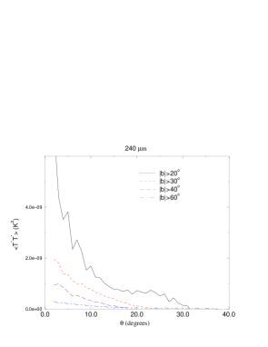
Figure 11: Angular correlation function at 240 $\mu$m.

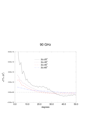
Figure 12: Predicted Galactic two-point correlations at 90 GHz at different zones.

The fluctuations, proportional to the square root of $\langle TT\rangle$, are about twice as high for $|b|>20^{\circ}$ than for $|b|>60^{\circ}$ at a scale of around $\theta=5^{\circ}$. Therefore, a decreasing fluctuation at higher latitudes is expected if the Galactic emission was the sole or at least an important contributor to the anisotropies. Perhaps the observed factor between $|b|>60^{\circ}$ and $|b|>20^{\circ}$ is not exactly two, since this quantity is subject to the errors of the calculations of the first and second factor, but the order of magnitude is something of this order and there is likely to exist a decreasing correlation with Galactic latitude.

In fact, MBRAs at microwave frequencies show a slightly decreasing dependence on $|b|$ with the fluctuations (Smoot et al. 1992, Fig. 2). They show that the correlations for $|b|>30^{\circ}$ and $|b|>40^{\circ}$ are nearly a half that for $|b|>20^{\circ}$ for angles $\theta$ less than 10^∘, although their first-year COBE-DMR data are quite noisy. Data showing this dependence more accurately are still awaited, specially when next experiments (PLANCK or MAP) be working. Until now, it cannot be said what exactly the $b$ dependence in the anisotropies at 90 GHz is.

Another conspicuous dependence is that the anisotropies in the southern Galactic hemisphere are higher than in the northern Galactic hemisphere. This is still not a proof against the Galactic predominance of anisotropies at microwave frequencies because the COBE-DMR survey also observes higher anisotropies in the southern Galactic hemisphere (see Fig. 1 of Bennett et al. 1996).

From this, the conclusion is that there is not a qualitative difference between the cosmological anisotropies and the cloud anisotropies. The position dependence of the MBRA is qualitatively similar in both microwaves and far infrared, so this may not be a proof neither for the cosmological origin nor for the Galactic origin.

3.5 Conclusions about possible Galactic predominance in MBRAs anisotropies

The conclusion is that under some particular, but not impossible, conditions, all the microwave background radiation anisotropies may be due to Galactic foregrounds rather than cosmological in origin. There are no arguments yet to exclude this possibility although this is not yet proved and the question remains open. A testable prediction of such a case would be that the amplitude of the fluctuations for $|b|>60^{\circ}$ would be about the half of that for $|b|>20^{\circ}$ for angles around 5 degrees.

The implications of such a question are extremely important, not merely for refining some quantity or other or for making certain corrections to get an accurate result for an individual parameter, but because it would result in a different qualitative description of the Universe. The implications for inflation theories or the formation of the large-scale structure of the Universe would be enormous, and our ideas regarding such formations would change completely. Hence, I think studying the influence of the Galaxy is a valuable exercise, in order to avoid the hazarding of cosmological theories based on cumulative errors, in which this paper claim to be still an open question.

4 Conclusions

The following main conclusions may be drawn from this paper:

• The extrapolation of anisotropies following the mean dust emission is a bad approximation since it does not take into account the growing contrast of colder clouds in the background of the diffuse interstellar medium. By considering this effect, it is found that dust thermal emission anisotropies are higher than expected by other authors, and that their amplitude is comparable to the observational data at 90 GHz.

• Our ignorance of the different emission mechanisms around 50 GHz (free-free, dust rotational emission, magnetic dipole emission from dust grains) do not allow the firm conclusion that anisotropies due to Galactic emission are not frequency dependent but this possibility remains open.

• If Galaxy-induced anisotropies are not responsible for the totality of the correlations they would at least be a non-negligible part of them, so untrustworthy cosmological conclusions could be reached from microwave background radiation anisotropy analysis unless possible Galactic emission processes are correctly subtracted.

• If the Galaxy-induced anisotropies made up the total correlations at microwave frequencies, then inflation, models of Galaxy formation and many parts of the standard cosmology would be wrong. This is not impossible, though there is no firm evidence either for or against it as yet.

- [1] Banday A. J., Wolfendale A. W., 1991, MNRAS 252, 462
- [2] Beichman C. A., 1987, ARA&A 25, 521
- [3] Bennett C. L., Banday A. J., Górski K. M., et al., 1996, ApJ 464, L1
- [4] Bennett C. L., Smoot G. F., Hinshaw G., et al., 1992, ApJ 396, L7
- [5] Bernardis P. de, Masi S., Melchiorri F., Melchiorri B., Vittorio N., 1992, ApJ 396, L57
- [6] Blitz L., 1991, in: Molecular clouds, R. A. James, T. J. Milla (eds.), Cambridge University Press, Cambridge, p. 49
- [7] Boggess N. W., Mather J. C., Weiss R., et al., 1992, ApJ 397, 420
- [8] Boulanger F., Abergel A., Bernard J. P., et al., 1996, A&A 312, 256
- [9] Boulanger F., Baud B., van Albada T., 1985, A&A 144, 9
- [10] Boulanger F., Pérault M., 1988, ApJ 330, 964
- [11] Burton W. B., Deul E. R., 1987, in: The Galaxy, G. Gilmore, B. Carswell, eds., Reidel, Dordrecht, p. 141
- [12] Bunn E. F., Hoffman Y. & Silk J., 1996, ApJ 464, 1
- [13] Celebonovic V., Samurovic S., Cirkovic M. M., 1997, Publ. Astron. Obs. Belgrade 57, 105
- [14] Combes F., Pfenninger D., 1997, A&A 327, 453
- [15] Condon J. J., Broderick J. J., Seielstad G. A., 1991, AJ 102, 2041
- [16] Condon J. J., Giffith M. R., Wright A. E., 1993, AJ 106, 1095
- [17] Condon J. J., Broderick J. J., Seielstad G. A., Douglas K., Gregory P. C., 1994, AJ 107, 1829
- [18] Cox P., Krügel E., Mezger P. G., 1986, A&A 155, 380
- [19] Davies R. D., Watson R. A., Gutiérrez C. M., 1996, MNRAS 278, 925
- [20] de Oliveira-Costa A., Kogut A., Devlin M. J., et al., 1997, ApJ 482, L17
- [21] de Oliveira-Costa A., Tegmark M., Page L. A., Boughn S. P., 1998, ApJ 509, L9
- [22] Draine B. T., 1994, in: The Infrared Cirrus and Diffuse Interstellar Clouds, ASP Conference Series 58, R. Cutri, W. B. Latters, eds., San Francisco, p. 227
- [23] Draine B. T., Lazarian A., 1998a, ApJ 494, L19
- [24] Draine B. T., Lazarian A., 1998b, preprint astro-ph/9807009
- [25] Draine B. T., Lee H. M., 1984, ApJ 285, 89
- [26] Femenía B., Rebolo R., Gutiérrez C. M., Limon M., Piccirillo L., 1998, ApJ 498, 117
- [27] Frisch P. C., York D. G., 1986, in: The Galaxy and the Solar System, R. Smoluchowski, J. N. Bahcall, M. S. Matthews, eds., University of Arizona Press, Tucson, p. 83
- [28] Fukushige T., Makino J., Ebisuzaki T., 1994, ApJ 436, L107
- [29] Gautier T. N. III, Boulanger F., Perault M., Puget J. L., 1992, AJ 103, 1313
- [30] Greenberg J. M., Li A., 1996, in: New Extragalactic Perspectives in the New South Africa, D. L. Block, J. M. Greensberg, eds., Kluwer, Dordrecht, p. 118
- [31] Guarini G., Melchiorri B., Melchiorri F., 1995, ApJ 442, 23
- [32] Gutiérrez C. M., Hancock S., Davies R. D., et al., 1997, ApJ 480, L83
- [33] Heiles C., 1976, ApJ 204, 379
- [34] Heiles C., Reach W. T., Koo B. C. 1988, ApJ 332, 313
- [35] Hinshaw G., Banday A. J., Bennett C. L., et al., 1996, ApJ 464, L25
- [36] Knox L., Scoccimarro R., Dodelson S., 1998, preprint astro-ph/9805012
- [37] Kogut A., 1997, AJ 114, 1127
- [38] Kogut A., Banday A. J., Bennett C. L., et al., 1996a, ApJ 460, 1
- [39] Kogut A., Banday A. J., Bennett C. L., et al., 1996b, ApJ 464, L5
- [40] Lagache G., Abergel A., Boulanger F., Puget J.-L., 1998, A&A 333, 709
- [41] Leitch E. M., Readhead A. C. S., Pearson T. J., Myers S. T., 1997, ApJ 486, L23
- [42] López-Corredoira M., Garzón F., Hammersley P. L., Mahoney T. J., 1998, MNRAS 301, 289
- [43] Low F. J., Cutri R. M., 1994, Infrared Phys. Technol. 35, 291
- [44] Magnani L., Blitz L., Mundi L., 1985, ApJ 295, 402
- [45] Masi S., Calisse P., de Bernardis P., et al., 1990, in: The Galactic and Extragalactic Background Radiation, IAU Symp. 139, S. Bowyer, C. Leinert, eds., Kluwer, Dordrecht
- [46] Mathis J. S., 1990, ARA&A 28, 37
- [47] Matsumoto T., Hayakawa S., Matsuo H., et al., 1988, ApJ 329, 567
- [48] Meinhold P., Clapp a., Devlin M., et al., 1993, ApJ 409, L1
- [49] Melchiorri F., Guarini G., Melchiorri B., Signore M., 1996, ApJ 464, 18
- [50] Melchiorri F., Melchiorri B. O., Ceccarelli C., Pietranera L., 1981, ApJ 250, L1
- [51] Pando J., Valls-Gabaud D. & Fang L.-Z., 1998, Phys. Rev. Lett. 81(21), 4568
- [52] Pfenninger D., Combes F., 1994, A&A 285, 94
- [53] Pfenninger D., Combes F., Martinet L., 1994, A&A 285, 79
- [54] Puget J. L., Abergel A., Bernard J. P., et al., 1996, A&A 308, L5
- [55] Puget J. L., Léger A., 1989, ARA&A 27, 161
- [56] Puget J. L., Léger A., Boulanger F., 1985, A&A 142, L19
- [57] Reach W. T., Dwek E., Fixsen D. J., et al., 1995, ApJ 451, 188
- [58] Reach W. T., Wall W. F., Odegard N., 1998, ApJ 507, 507
- [59] Readhead A. C. S., Lawrence C. R., 1992, ARA&A 30, 653
- [60] Reich W., 1982, A&AS 48, 219
- [61] Reich P., Reich W., 1986, A&AS 63, 205
- [62] Reynolds R. J., 1991, ApJ 372, L17
- [63] Schaefer J., 1994, A&A 284, 1015
- [64] Schaefer J., 1996, Europhys. Lett. 34(1), 69
- [65] Schlegel D. J., Finkbeiner D. P., Davis M., 1998, ApJ 500, 525
- [66] Schloerb F. P., Snell R. L., Schwartz P. R., 1987, ApJ 319, 426
- [67] Scoville N. Z., Sanders D. B., 1986, in: The Galaxy and the Solar System, R. Smoluchowski, J. N. Bahcall, M. S. Matthews, eds., University of Arizona Press, Tucson, p. 69
- [68] Smoot G. F., 1998, preprint astro-ph/9801121
- [69] Smoot G. F., Bennett C. L., Kogut A., et al., 1992, ApJ 396, L1
- [70] Sodroski T. J., Odegard N., Arendt R. G., et al., 1997, ApJ 480, 173
- [71] Suginohara M., Suginohara T., Spergel D. N., 1998, ApJ 495, 511
- [72] Tegmark M., 1998, ApJ 502, 1
- [73] Wheelock S. L., Gautier T. N., Chillemi J., et al., 1994, IRAS Sky Survey Atlas: Explanatory Supplement, Jet Propulsion Laboratory, Pasadena
- [74] White M., Scott D., Silk J., 1994, ARA&A 32, 319
- [75] Wright E. L., 1993, in: Back to the Galaxy, AIP Conf. Proc. 278, S. S. Holt, F. Verter, eds., AIP, New York, p. 193
- [76] Wright E. L., 1998, ApJ 496, 1
- [77] Wright E. L., Mather J. C., Bennett C. L., et al., 1991, ApJ 381, 200