The 2dF Galaxy Redshift Survey: Spectral Types and Luminosity Functions

Abstract

We describe the 2dF Galaxy Redshift Survey (2dFGRS), and the current status of the observations. In this exploratory paper, we apply a Principal Component Analysis to a preliminary sample of 5869 galaxy spectra and use the two most significant components to split the sample into five spectral classes. These classes are defined by considering visual classifications of a subset of the 2dF spectra, and also by comparing to high quality spectra of local galaxies. We calculate a luminosity function for each of the different classes and find that later-type galaxies have a fainter characteristic magnitude, and a steeper faint-end slope. For the whole sample we find $M^{\star}=-19.7$ (for $\Omega$=1,$H_{0}$=100 km s^-1 Mpc^-1), $\alpha=-1.3$, $\phi^{\star}=0.017$. For class 1 (‘early-type’) we find $M^{\star}=-19.6$, $\alpha=-0.7$, while for class 5 (‘late-type’) we find $M^{\star}=-19.0$, $\alpha=-1.7$. The derived 2dF luminosity functions agree well with other recent luminosity function estimates.

1 INTRODUCTION

The 2dF Galaxy Redshift Survey (2dFGRS; Colless 1998, Maddox 1998) is a major new redshift survey utilising the full capabilities of the 2dF multi-fibre spectrograph on the Anglo-Australian Telescope (AAT). The observational goal of the survey is to obtain high quality spectra and redshifts for 250,000 galaxies to an extinction-corrected limit of $b_{J}$=19.45. The survey will eventually cover approximately 2000 $\Box^{\circ}$, made up of two continuous declination strips plus 100 random 2°-diameter fields. One strip is in the southern Galactic hemisphere and covers approximately 75°$\times$15° centred close to the South Galactic Pole at ($\alpha$,$\delta$)=($01^{h}$,$-30$°); the other strip is in the northern Galactic hemisphere and covers 75°$\times$7.5° centred at ($\alpha$,$\delta$)=($12.5^{h}$,$+00$°). The 100 random fields are spread uniformly over a 7000 $\Box^{\circ}$ region in the southern Galactic cap.

The survey has been designed to provide a detailed picture of the large-scale structure of the galaxy distribution in order to understand structure formation and evolution and to address cosmological issues such as the nature of the dark matter, the mean mass density of the universe, the role of bias in galaxy formation and the Gaussianity of the initial mass distribution. However the survey will also yield a comprehensive database for investigating the properties of the low-redshift galaxy population, providing: $b_{J}$ and $r_{F}$ magnitudes and various image parameters from the blue and red Southern Sky Survey plates scanned with the Automatic Plate Measuring machine (APM); moderate quality spectra (S/N$\mathrel{\hbox{\hbox to0.0pt{\hbox{\lower 4.0pt\hbox{$\sim$}}\hss}\hbox{$>$}}}$10 per $4.3\AA$ pixel); derived spectroscopic quantities such as redshifts and spectral types.

The first test observations for the 2dFGRS were taken at the start of the 2dF instrument commissioning period in November 1996. The first survey observations with all 400 fibres were obtained in October 1997, and as of March 1999 we have measured over 40,000 redshifts. We plan to complete the survey observations by the end of 2000.

This paper presents some of the first results from the 2dFGRS. It deals with the Principal Component Analysis (PCA) methods that we are developing for classifying galaxy spectra, and the application of these methods to deriving the luminosity functions for different galaxy spectral types. The luminosity function (LF) is a fundamental characterization of the galaxy population. It has been measured from many galaxy surveys with differing sample selections, covering a wide range of redshifts. Generally a Schechter function (Schechter 1976),

$$\phi(L)dL=\phi^{\star}({L\over L^{\star}})^{\alpha}exp(-{L\over L^{\star}}){dL\over L^{*}},$$ (1)

with

$${L\over L^{\star}}=10^{0.4(M^{\star}-M)}$$ (2)

provides a good fit to field galaxy data, but the parameters $M^{\star}$, $\alpha$ and $\phi^{*}$ are still relatively uncertain.

Surveys of bright field galaxies, such as the CfA2 (Marzke et al 1994) and SSRS2 (Marzke & Da Costa 1997) have mean redshift $\bar{z}\sim 0.02$ and so cover relatively small volumes. This leads to a large sample variance on these measurements. Also they are based on photometric catalogues which have been visually selected from photographic data, which makes selection biases hard to quantify. Deeper surveys such as the CFRS (Lilly et al 1995), and AUTOFIB (Ellis et al 1996) surveys are based on better controlled galaxy samples, but the sample volumes are very small, and they reach to much higher redshifts ($z\sim 1$), so that galaxy evolution is an important factor.

The Stromlo-APM Redshift Survey (SAPM, Loveday et al 1992) the Las Campanas Redshift Survey (LCRS; Lin et al 1996) and the ESO Slice Project (ESP; Zucca et al 1997) cover intermediate redshifts, $z\sim 0.05-0.2$, and give the most reliable current estimates of the local luminosity function. The estimated values of $M^{*}$ from these surveys agree to about 0.1 magnitude, and $\phi^{*}$ varies by a factor of $\sim$ 1.5. The faint-end slope, $\alpha$, is more poorly determined, ranging from $-0.7\pm 0.05$ for the LCRS to $-1.22^{+0.06}_{-0.07}$ for the ESP. Some of these differences are likely to be due to sample variance, but some may be due to different selection effects in the surveys, e.g, the high surface brightness cut imposed on the LCRS survey. The 2dF survey reaches to a similar depth, will cover a much larger volume than the LCRS survey, and so have smaller sample variance, allowing us to estimate luminosity functions for several sub-samples of galaxies. The mean surface brightness isophotal detection limit of the underlying APM catalogue is $b_{j}=25$.

It is well established that the galaxy luminosity function depends on the type of galaxy that is sampled. Morphologically late-type galaxies tend to have a fainter $M^{*}$ (in the B-band) and steeper faint-end slope, $\alpha$, (Loveday et al. 1992, Marzke et al 1998). Spectroscopically, selecting galaxies with higher [OII] equivalent width leads to a similar trend (Ellis et al. 1996, Lin et al 1996), as does the selection of bluer galaxies (Marzke & Da Costa 1997, Lin et al 1996). These results reflect the correspondence between spectral and morphological properties, with galaxies of late type morphology having stronger emission lines and bluer continuum than galaxies of early type morphology. However this correspondence is quite approximate and a considerable scatter exists.

In this paper we use a classification scheme based on PCA of the galaxy spectra (e.g. Connolly et al. 1995; Folkes, Lahav & Maddox 1996; Sodré & Cuevas 1997; Galaz & de Lapparent 1998; Bromley et al. 1998; Glazebrook, Offer & Deeley 1998; Ronen, Aragón-Salamanca & Lahav 1999). This provides a representation of the spectra in two (or more) dimensions that highlights the differences between individual galaxies. The technique is based on finding the directions in spectral space in which the galaxies vary most, and so offers an efficient, quantitative means of classification. Bromley et al (1998) have studied the variation of the LCRS LF with spectral type using classes from a similar PCA technique. They find that late type galaxies have a steeper faint-end slope than early type galaxies. They also find a clear density-morphology relation: over half of their extreme early-type objects are found in regions of high density, whereas these regions contain less than a quarter of their extreme late-type objects.

The plan of the paper is as follows. In §2 we briefly summarise the construction of the survey source catalogue, the capabilities of the 2dF multi-fibre spectrograph, the observing and reduction procedures employed and the main properties of the subset of the data which will be used in the rest of the paper. In §3 we outline the fundamentals of Principal Component Analysis, describe the steps required to prepare the spectra, and then present the principal components for our sample of galaxy spectra and their distribution. Two methods to connect the PCA decomposition of a galaxy’s spectrum with its physical (spectral or morphological) type are investigated in §4. We then define spectral types based on the PCA decomposition and use these types to derive K-corrections for each galaxy in our sample. The luminosity functions (LFs) for the whole sample, and for each spectral type separately, are derived in §5, using both a direct estimator and a parametric method. Our results are discussed in §6, focusing on the strengths and weaknesses of the PCA spectral classifications and a comparison of the LFs for our spectral types with similar analyses in the literature.

2 THE DATA

2.1 Source catalogue

The source catalogue for the survey is a revised and extended version of the APM galaxy catalogue (Maddox et al. 1990a,b,c). This catalogue is based on APM scans of 390 IIIa-J plates from the UK Schmidt Telescope (UKST) Southern Sky Survey. The magnitude system for the Southern Sky Survey is defined by the response of Kodak IIIa-J emulsion in combination with a GG395 filter, zero pointed using Johnson B band CCD photometry. The extended version of the APM catalogue includes over 5 million galaxies down to $b_{J}$=20.5 in both north and south Galactic hemispheres over a region of almost 10⁴ $\Box^{\circ}$ (bounded approximately by declination $\delta$$\leq$+3° and Galactic latitude $|b|$$\mathrel{\hbox{\hbox to0.0pt{\hbox{\lower 4.0pt\hbox{$\sim$}}\hss}\hbox{$>$}}}$20°). The astrometry for the galaxies in the catalogue has been significantly improved, so that the rms error is now 0.25″ for galaxies with $b_{J}$=17–19.45. Such precision is required in order to minimise light losses with the 2″ diameter fibres of 2dF. The photometry of the catalogue is calibrated with numerous CCD sequences and has a precision (random scatter) of approximately 0.2 mag for galaxies with $b_{J}$=17–19.45. The mean surface brightness isophotal detection limit of the APM catalogue is $b_{j}=25$. The star-galaxy separation is as described in Maddox et al. (1990b), supplemented by visual validation of each galaxy image. A full description of the source catalogue is given in Maddox et al. (1998, in preparation).

2.2 The 2dF multi-fibre spectrograph

The 2dF facility consists of a prime focus corrector, a focal plane tumbler unit and a robotic fibre positioner, all mounted on an AAT top-end ring which also supports the two spectrographs.

The 2dF corrector introduces chromatic distortion (i.e, shifts between the blue and red images). This is a function of radius and is, by design, a maximum at the halfway point (radius=30 arcmin) and minimum at the centre and edge.

The absolute shifts, at a particular wavelength, are allowed for in the 2dF configuration program and for our survey we configure for 5800Å. Relative to this we have maximum residual shifts of +0.9 arcsec (at 4000Å) and -0.3 arcsec (at 8000Å). The typical shift, averaged over the field, will be of order half these values (Bailey and Glazebrook 1998).

The 2dF instrument has two field plates and two full sets of 400 fibres. This allows one plate to be configured while observations are taking place with the other. The robotic positioner uses a gripper head which places magnetic buttons containing the fibre ends at the required positions on the plate. When the plate is prepared and one set of observations are complete, the tumbler can rotate to begin observations on the new field. Each field plate has 400 object fibres and an additional 4 guide-fibre bundles, which are used for field acquisition and tracking. The object fibres are 140 $\mu$m in diameter, corresponding to about 2.16″ at the centre and 2″ at the edge of the field. Two identical spectrographs receive 200 fibres each and spectra are recorded on thinned Tektronix 1024 CCDs.

Further detail on the design and use of the instrument is given in Bailey & Glazebrook (1999), Lewis et al. (1998) and Smith & Lankshear (1998).

In terms of spectral analysis, the design of the system has a number of implications. Firstly, all 400 spectra taken in a particular observation have the same integration time, regardless of the brightness of individual targets. After the fibre feed, each of the two sets of 200 spectra pass through an identical optical system, which ensures some consistency. The combination of the fibre size, small positioning errors and chromatic variation means that, particularly for nearby extended objects, the observed spectrum is not necessarily representative of the whole object. The impact of some of these effects is examined in more detail below.

2.3 Observations and reductions

This paper uses only the data taken for the 2dFGRS in two early observing runs: 1997 October 29 to 1997 November 3 and 1998 January 23–29. In the former we observed 14 2dF fields and 3882 galaxies; in the latter we observed 16 2dF fields and 4482 galaxies. Counting repeats only once this gives a total of 7972 galaxies. The 400 fibres in each field were shared between the targets of the 2dFGRS and the 2dF QSO Redshift Survey (Boyle 1998). The observations were performed with the 300B gratings, giving an observed wavelength range of approximately 3650Å to 8000Å, although this varies slightly from fibre to fibre. The spectral scale was 4.3Å/pixel and the FWHM resolution measured from arc lines was 1.8-2.5 pixels (varying over the wavelength range).

The exposure time for the observations described here was around 70 min. This time was determined by the time necessary for configururation of the fibres (with improvement in the configuration time, the observation time has been reduced to around 60 min). The spectra were reduced using an early version of the 2dfdr pipeline software package (Bailey & Glazebrook 1999). Typically, three to four sub-exposures were taken and cosmic rays removed by a sigma-clipping algorithm. Galaxies at the survey limit of $b_{J}$=19.45 have a median S/N of $\sim 14$, which is more than adequate for measuring redshifts and permits reliable spectral types to be determined, as described below.

Redshifts were found by two independent methods: the first, cross-correlating the spectra with absorption line templates, and the second, by emission line fitting. These automatic redshift estimates were then confirmed by visual inspection of each spectrum, and the more reliable of the two results chosen as the final redshift. A quality flag (Q) was manually assigned to each redshift: Q=3 and Q=4 (7180 objects) correspond to reliable redshift determinations; Q=2 (574 objects) means a probable redshift; and Q=1 (218 objects) means no redshift could be determined. We note that some stars enter the sample because the star-galaxy classification criteria for the source catalogue are chosen to exclude as few galaxies as possible, at the cost of 4% contamination of the galaxy sample by stars. As a crude criterion, and for the purpose of this work, we consider all objects with $z<0.01$ as stars. Only the 6899 non-stellar objects with quality flag Q=3 or Q=4 are included in subsequent analysis. Using this criterion, the sample of galaxies with reliable redshifts is 90% of all observed objects not identified as stars. We note that more recent observations are giving a higher redshift completeness.

It is worth noting that PCA and redshift determination can be performed simultaneously in a single procedure which can improve the redshift determination by reducing its dependency on a predetermined set of template spectra (Glazebrook et al. 1998). We are investigating future use of this method.

The fields observed in these two runs lie in the northern and southern declination strips covered by the survey. Note that at the median redshift of the sample, $\hat{z}=0.1$, 2° corresponds to a comoving distance of 9.7 h^-1 Mpc. Figure 1 summarises some of the properties of this sample. The distribution in apparent magnitude and redshift is shown in Figure 1a; the median redshift of the galaxies increases from $\hat{z}=0.07$ at $b_{J}$=17 to $\hat{z}=0.14$ at $b_{J}$=19.45. The redshift distribution in Figure 1c shows considerable clustering in redshift space, reflecting in part that our survey is still dominated by a few lines-of-sight whcih intersect common structures. We expect this to average out when we complete the full volume.

Figure 1: Properties of the sample: (a) the distribution of redshifts as a function of apparent magnitude; (b) the differential number counts; (c) the redshift distribution.

Figure 2 shows the redshift completeness, as a function of apparent magnitude, computed as the fraction of objects with good redshift ($Q>2$) out of all observed objects.

A further completeness factor must also be included to allow for the fact that not all galaxies in the photometric catalogues can be assigned a fibre in the 2dF configurations. One of the constraints on the configuration is the fact that two fibres cannot be put closer than $25^{\prime\prime}$, for the most favourable geometry. The tiling process of the fields is designed to maximise the completenes of the survey as galaxies in close pairs can be observed in diffrent tiles. The final completeness is extremely high (93%).

Figure 2: The fraction of objects for which reliable redshifts were obtained over all observed objects.

3 PRINCIPAL COMPONENT ANALYSIS

3.1 The method

A spectrum, like any other vector, can be thought of as a point in an $M$-dimensional parameter space. One may wish for a more compact description of the data. This can be accomplished by Principal Component Analysis (PCA), a well-known statistical tool that has been used in a number of astronomical applications (Murtagh & Heck 1987). By identifying the linear combination of input parameters with maximum variance, PCA finds the principal components that can be most effectively used to characterise the inputs.

The formulation of standard PCA is as follows. Consider a set of $N$ objects ($i=1,N$), each with $M$ parameters ($j=1,M$). If $r_{ij}$ are the original measurements of these parameters for these objects, then mean subtracted quantities can be constructed,

$$X_{ij}=r_{ij}-{\bar{r}_{j}}\ ,$$ (3)

where ${\bar{r}_{j}}={1\over N}\sum_{i=1}^{N}r_{ij}$ is the mean. The covariance matrix for these quantities is given by

$$C_{jk}={1\over N}\sum_{i=1}^{N}X_{ij}X_{ik}\hskip 14.22636pt1\leq j\leq M\hskip 14.22636pt1\leq k\leq M\ .$$ (4)

It can be shown that the axis (i.e, direction in vector space) along which the variance is maximal is the eigenvector ${\bf e_{1}}$ of the matrix equation

$$C{\bf e_{1}}=\lambda_{1}{\bf e_{1}}\ ,$$ (5)

where $\lambda_{1}$ is the largest eigenvalue (in fact the variance along the new axis). The other principal axes and eigenvectors obey similar equations. It is convenient to sort them in decreasing order (ordering by variance), and to quantify the fractional variance by $\lambda_{\alpha}/\sum_{\alpha}\lambda_{\alpha}$. The matrix of all the eigenvectors forms a new set of orthogonal axes which are ideally suited to an efficient description of the data set using a truncated eigenvector matrix employing only the first $P$ eigenvectors

$$U_{P}=\{e_{jk}\}\hskip 28.45274pt1\leq k\leq P\hskip 28.45274pt1\leq j\leq M\ ,$$ (6)

where $e_{jk}$ is the $j$th component of the $k$th eigenvector. The turncation turns out to be efficient because as it happens the cloud of points which represent the spectra closely lies in a low dimensional sub-space. This can be seen from the fact that the first few eigenvalues account for most of the variation in the data, and it can also be seen that the higher eigenvectors contain mostly the noise (Folkes, Lahav & Maddox, 1996).

Now if a specific spectrum is taken from the matrix defined in Equation 3, or possibly a spectrum from a different source which has been similarly mean-subtracted and normalised, it can be represented by the vector of fluxes ${\bf x}$. The projection vector ${\bf z}$ onto the $M$ principal components can be found from (here ${\bf x}$ and ${\bf z}$ are row vectors):

$${\bf z}={\bf x}U_{M}\ .$$ (7)

Multiplying by the inverse, the spectrum is given by

$${\bf x}={\bf z}{U_{M}}^{-1}={\bf z}{U_{M}}^{t}\ ,$$ (8)

since $U_{M}$ is an orthogonal matrix by definition. However, using only $P$ principal components the reconstructed spectrum would be

$${\bf x}_{rec}={\bf z}{U_{P}}^{t}\ ,$$ (9)

which is an approximation to the true spectrum.

The eigenvectors into which we project the spectra can be viewed as ‘optimal filters’ of the spectra, in analogy with other spectral diagnostics such as colour filter or spectral index. Finally, we note that there is some freedom of choice as to whether to represent a spectrum as a vector of fluxes or of photon counts. The decision will affect the resulting principal components, as a representation by fluxes will give more weight to the blue end of a spectrum than a representation by photon counts. In this paper all spectra are represented as photon counts, but we leave open the question of which representation is ‘the best’ in some sense.

3.2 Data preparation

Before we can carry out Principal Component Analysis a number of procedures are required to prepare the spectra.

Firstly, residuals from strong sky lines and bad columns were removed by interpolating the continuum across them. Secondly, we corrected for sky absorption at the A and B bands (7550Å to 7700Å and 6850Å to 6930Å  respectively) as follows: the spectrum was smoothed with a 150Å Gaussian filter to give the low-resolution spectral shape, and with a 3Å Gaussian filter to give a noise-reduced spectrum closely following the shape of the absorption band profiles. The original spectrum was then multiplied by the ratio of the former to the latter over the spectral ranges covered by the atmospheric absorption bands.

The system response also needs to be removed from the spectra. This was done by calculating a second-order polynomial fit to the 2dF system response with the 300B grating from observations of Landolt standard stars in BVR. The fit can be seen in Figure 3. Some fibre-to-fibre variations in the response function can be expected, as well as possible time variations. We have observed wavelength dependent variations at the level of 20%. We expect improvement in this with the application of an improved extraction algorithm (not applied to the data presented here). It is possible to remove such unknown variations in the flux calibration by, e.g., by removing the low frequency Fourier components, as was done by Bromley et al. (1998). However such a procedure will also remove potentially important information inherent in the continuum. Therefore, in this paper, we chose to use our measured flux calibration and retain the whole spectrum. We leave it for a future study to compare the two approaches.

Figure 3: Fitted response function for the 2dF system, based on observations of Landolt standard stars.

The next step is to de-redshift the spectra to their rest frame and re-sample them to a uniform spectral scale with 4Å bins. Since the galaxies cover a range in redshift, the rest-frame spectra cover different wavelength ranges. To overcome this problem, only the 6015 objects with redshifts in the range 0.01$\leq$$z$$\leq$0.2 are included in the analysis. All the objects meeting this criterion then have rest-frame spectra covering the range 3700Å to 6650Å (the lower limit was chosen to exclude the bluest end of the spectrum where the response function is poor). Limiting the analysis to this common wavelength range means that all the major optical spectral features between [OII] (3727Å) and H$\alpha$ (6563Å) are included in the analysis. In order to make the PCA spectral classifications as robust as possible, objects with redshifts but relatively low S/N were eliminated by imposing a minimum mean flux of 50 counts per bin. The spectra are then normalised so that the mean flux over the whole spectral range is unity. Figure 4 shows examples of the prepared spectra for a range of galaxy types, with some of the major spectral features indicated. The spectral classifications and luminosity functions are derived from this final sample of 5869 galaxies, each described by 738 spectral bins.

Finally, we reiterate that we applied the PCA analysis to the spectra given as photon counts per bin, as opposed to energy flux per bin.

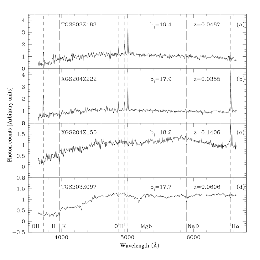
Figure 4: Examples of 2dF spectra prepared for PCA analysis. Sky lines and bad columns have been interpolated over, atmospheric absorption features corrected and the instrument response function divided out. The spectra have then been transformed to the rest-frame, re-sampled to 4Å bins over the limited range 3700Å to 6650Å, and normalised to unit mean flux.

3.3 Application

Principal Component Analysis of the sample spectra was carried out by finding the eigenvectors (principal components) of the covariance matrix of the de-redshifted and mean subtracted spectra. The mean spectrum and first three principal components (PCs) can be seen in Figure 5. The first PC accounts for 49.6% of the variance in the sample, the second accounts for 11.6%, and the third accounts for 4.6%. This still leaves 34.2% of the variance for the later PCs. Much of this remaining variance will be due to noise in the data—compare the distribution of variance over the principal components with that seen in the PCA of synthetic spectra by Ronen et al. (1999) or high S/N observations by Folkes (1998). The 1st PC shows the correlation between a blue continuum slope and strong emission-line features. The 2nd PC allows for stronger emission lines without a strong continuum shape. The 3rd PC allows for an anti-correlation between the oxygen and H$\alpha$ lines, relating to the ionization level of the emission-line regions.

Figure 5: The mean spectrum and first three principal components for the sample spectra. Note that the sign of the PCs is arbitrary.

Figure 6 shows the distribution of the sample spectra in the PC1–PC2 plane. The spectra form a single cluster, with the blue objects with emission lines found to the right of the plot and the red objects with absorption lines to the left. Objects with particularly strong emission lines are found lower on the plot. We expect that there exists some small scatter due to Poisson noise, but this is suppressed due to the noise reduction property of the PCA technique. Errors in the flux calibration will cause a systematic error, while fibre-to-fibre variations and changes from run to run could introduce additional random scatter (see Ronen et al. (1999) and Folkes (1998) for a discussion of errors due to Poisson noise and flux calibration). For this reason, Bromley et al. (1998) chose to high-pass filter the spectra. However this involves loss of information, which we regard as undesirable. The accuracy of the 2dF flux calibration is currently being examined, and will be included in the final analysis of 2dF data.

We will use the location of spectra in the PC1–PC2 plane as the basis of our spectral classification scheme. We have investigated the variation in the distribution of objects in the PC1–PC2 plane as a function of various parameters (see Folkes, 1998). We find that there is very little difference in the distribution with galaxy size or ellipticity. There is a small variation with redshift, in that there is a population of low luminosity galaxies with very strong emission lines at low redshift which are not seen at higher redshifts.

4 SPECTRAL CLASSIFICATION

Principal Component Analysis has revealed the main features of the galaxy spectra, but without some further information it is not clear how to segment the PC1–PC2 plane into spectral classes, whether such a classification is meaningful, and what the physical significance of such classes would be. Two approaches were used in combination to gain insight into the distribution of the galaxy spectra in principal component space. One was to classify a subsample of the spectra by eye using a simple phenomenological scheme, and hence look at the distribution of galaxies with specific spectral features in the PC space. The second was to take the Kennicutt (1992) sample of spectra belonging to galaxies of known structural morphology and project them onto the PC1–PC2 plane. A third approach , to relate the PCs to physical parameters (e.g. age, metallicity and star-formation history of galaxies) by using model spectra, is discussed in Ronen et al. (1999).

4.1 Spectral features

A simple 3-parameter classification scheme was used to identify spectral features. The scheme allocates each galaxy spectrum a code number from 0 to 2 according to the strength of spectral features in each of the following three categories: early-type absorption lines (molecular features such as H, K, CN, Mg), Balmer series absorption lines (H$\gamma$, H$\delta$, etc.), and nebular emission lines (OII, OIII, H$\beta$ etc.). This is physically motivated by the typical features produced by stellar populations at progressive stages during and after star-formation. We have selected an unbiased subsample of 56 galaxies which were classified using this scheme, and then collected into six broad classes with physical motivation, as follows: Class A, strong absorption lines; Class B, weak absorption lines; Class C, weak features; Class D, strong balmer lines; Class E, strong emission lines; Class F, Strong Balmer and Emission lines. We note that these classes are not directly related to any structural morphology.

The 56 example objects can be plotted on the PC1–PC2 plane. These can be seen in Figure 6, which shows considerable segregation on the PC1–PC2 plane. The Class A objects, representing the strong absorption line systems with old stellar content and little star formation inhabit a clear region of the plots. The Class B, weaker absorption line systems also show a clear cluster. Classes D, E and F with emission and/or Balmer lines inhabit the lower sections of the plot in fairly distinct areas. The Class C objects that do not have particularly prominent features in absorption or emission are more widely spread.

Figure 6: The distribution of galaxy spectra in the PC1–PC2 plane, with the visual classifications based on spectral features overlaid for a subset of the objects.

Although some segregation is shown in the PC1–PC3 plane, in general PC3 is not such a good discriminator, as shown in Figure 7. However it does allow good separation of the Balmer and oxygen emission line objects, since PC3 allows for an anti-correlation between those lines.

Figure 7: The distribution of galaxy spectra in the PC1–PC3 plane, with the visual classifications based on spectral features overlaid for a subset of the objects.

4.2 Galaxy morphology

In the second approach, the 55 Kennicutt (1992) galaxies were split into five standard morphological groups (E/S0, Sa, Sb, Scd, Irr) plus 29 objects with unusual spectra. To make use of this set of well-fluxed, reliable spectra of known morphology, they need to be projected onto the PC space defined by the 2dF spectra. To do this, each Kennicutt galaxy is de-redshifted to its rest frame then smoothed with a 3Å Gaussian filter, which (by experimentation) gives a line profile similar to that of the 2dF spectra. The Kennicutt spectra are then sampled with 4Å bins across the same wavelength range and normalised in the same way as the 2dF data. The remaining uncertainties are due to any systematic errors in the 2dF response function.

The 55 Kennicutt galaxies prepared in this way were then projected onto the PCs from the 2dF sample. Figure 8 shows the PC1–PC2 plane with the Kennicutt points labeled by morphological group. This figure clearly shows the progression in morphological type across the plot, with the many unusual objects, such as star-bursts and irregulars populating the extreme emission-line regions. The Seyfert galaxies from the Kennicutt sample fall below the morphological sequence of normal galaxies, since they have emission lines that are not necessarily associated with a blue continuum. However many of the other unusual galaxies with star-burst activity also fall in this area, so that the Seyferts are not clearly segregated. Figure 6 shows that this area is populated by the Balmer strong objects and some of the Class 3 survey spectra, which show a variety of weak absorption and emission features.

Figure 8: The distribution of the sample spectra in the PC1–PC2 plane. The positions of the Kennicutt sample galaxies are overlaid. The lines divide the plane into the five spectral classes we have adopted, with type 1 objects towards the top left of the plane and type 5 objects towards the bottom right.

4.3 Definition of spectral types

It is now possible to define sensible classifications in PC space based on meaningful spectral and morphological classifications. Here we wish to emphasise the links between galaxy spectra and morphology, so we choose to employ parallel cuts in the PC1–PC2 plane along the Hubble sequence as delineated by the Kennicutt galaxies. The cuts can be seen in Figure 8 with the Kennicutt galaxies superimposed. This defines five spectral types, which are roughly analogous to the five morphological groups. The Kennicutt galaxies do not seem to fall in the region where most of the 2dF galaxies are, and this may be due to the selection bias of the sample, but also due to flux calibration. With this reservation, the exact placement of the lines on Figure 8 is somewhat arbitrary, but we have used both the projection of the Kennicutt galaxies and our by-eye spectral classification to place the lines as appropriately as possible. Note, however, that there is no one-to-one correspondence between these five classes and the six classes described in section 4.1. To check the robustness of our object classification in view of the fact that the response function is fibre dependent, we have examined 212 objects with repeated observations in overlapping fields. We find that 64% of the repeated objects have the same class, and 95% have the same class to within one type.

The mean spectra for each of the five types defined by these cuts are shown in Figure 9. This shows the clear progression from the red absorption-line spectrum of Type 1 to the strong emission-line spectrum of Type 5. As can be seen from Figure 8, there is not a one-to-one relation between morphology and spectral type, but the general relation is clear. The mean spectra are in good agreement with the spectra of the equivalent morphological groups given by Pence (1976), Coleman et al. (1980) or Kennicutt (1992): Type 1 corresponds approximately to E/S0 galaxies, Type 2 to Sa galaxies, Type 3 to Sb galaxies, Type 4 to Scd galaxies and Type 5 to the irregulars. The agreement is excellent in the blue end ($\lambda<5000\AA$), though towards the red end the spectra of the 2dF types have less flux than the corresponding Pence spectra. This is probably due to inaccuracies in the current preliminary flux calibration, and we will be making further observations to improve the mean calibration of the 2dF spectra. We note that, in principle, the PCs can be used as continuous variables, without binning them.

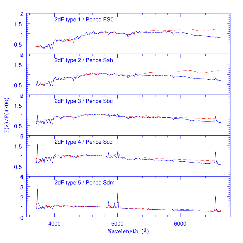
Figure 9: The mean spectrum for each spectral type (solid line), compared with the corresponding Pence (1976) type (dashed line).

4.4 K-corrections

Spectral types are of intrinsic interest, but are also important in that they yield the K-corrections necessary for estimating absolute magnitudes. The K-correction appropriate to a particular galaxy could in principle be obtained directly from the observed spectrum, from its PCA reconstruction, or from its principal components as $K(z,{\rm PC1},{\rm PC2},\ldots)$. These approaches require careful examination of a number of issues including the extent to which the fibre spectrum is representative of the integrated galaxy spectrum, the systematic uncertainties in the flux calibration and the available wavelength range (cf Heyl et al, 1997). A further complication with our current analysis is that we have limited the PCA to a fixed range in rest-frame wavelength, 3700Å to 6650Å. Since the $b_{J}$ pass-band extends from $3950$Åto $5600$Å, the wavelength range of the PCA reconstruction, or the class mean spectra allow us to calculate K-corrections in $b_{J}$ only for galaxies $z<0.07$.

In light of these complications we adopt here a practical approach, associating the spectral types defined in the previous section with specific template spectral energy distributions (SEDs). As discussed above, the SEDs of the five morphological types given by Pence (1976) agree well (i.e, at the blue end, which is that relevant for the $b_{J}$ filter) with the mean spectra of our five spectral types. We therefore identify our spectral types with Pence’s SEDs. We compute the appropriate K-corrections from Pence’s tabulations, transforming the K-corrections in the B and V filters according to the colour relation given by Blair & Gilmore (1982) for the $b_{J}$ filter,

$$K(b_{J})=K(B)-0.28(K(B)-K(V))\ .$$ (10)

The K-corrections derived in this way for the redshift range $0<z<0.2$ are shown as the curves in Figure 10.

Figure 10: K-corrections for the $b_{J}$ filter derived from values given in Pence (1976) for B and V filter K-corrections.

5 THE GALAXY LUMINOSITY FUNCTION

5.1 Methods

Figure 11: Luminosity functions including K-corrections and weighting to compensate for incompleteness. Points show 1/$V_{\rm max}$ estimates with Poisson error bars. This method assumes a uniform distribution, which is unlikely to be the case in our rather small survey volume. The line is a Schechter function fit by the parametric STY maximum likelihood method. The normalisations for the two methods are derived separately (see text). The number of galaxies of each type is indicated in the fourth line in each box. We used $\Omega$=1 and $H_{0}$=100 km s^-1 Mpc^-1.

In computing the luminosity functions (LFs) we use both the 1/$V_{\rm max}$ method (Schmidt 1968) for a non-parametric estimate of the LF and the STY method (Sandage, Tammann & Yahil 1979) for a maximum likelihood fit of LF parameters. The statistical properties of these different estimators are discussed by Felten (1976), Efstathiou, Ellis & Peterson (1988) and Willmer (1997). The 1/$V_{\rm max}$ method assumes uniform spatial distribution, while the STY method assumes a parametric form, here taken to be a Schechter function (Schechter 1976). The use of other LF estimators is left for future work. We assume the cosmological parameters to be $\Omega=1$ and $\Lambda=0$ (hence $q_{0}=\frac{1}{2}$) and $H_{0}$=100 km s^-1 Mpc^-1.

The analysis is limited to $z<0.2$ by the definition of the sample used in the PCA. The effective area of the survey can be estimated by dividing the number of objects currently observed by the final expected density. The density of galaxies brighter than $b_{J}=19.45$ as derived from the parent 2dFGRS source catalogue is $180/\hbox{\,$\Box^{\circ}$}$. Taking into account a configuration completeness of 93%, the effective area for the 7972 galaxies observed is $47.3\hbox{\,$\Box^{\circ}$}$. This provides the overall normalisation for our LF estimates.

We also define a completeness factor for each apparent magnitude range in the currently observed sample compared to the parent photometric sample, and weight each galaxy accordingly in our LF estimates. We note that there may be selection biases that may depend on spectral type (e.g, because of surface brightness effects and also because at low S/N emission line galaxies are easier to measure redshfits for). However it is not possible to account for such spectral type dependency in the completeness since, by defintion, the partition into classes is known only for our selected sample classified spectra and not for the parent catalogue.

Error estimates for the 1/$V_{\rm max}$ LFs are computed assuming Poisson statistics to deduce the fractional error without weights, then applying that fractional error to the actual estimate of the LF. These errors are under-estimates since they neglect the effects of clustering, which will be especially apparent at the faint end of the LFs, where the galaxies are sampled over a relatively small volume.

Error estimates for the parameters obtained by the STY method are found using the $\chi^{2}$ contours of the likelihood ratio distribution. Note that the fact that the sample is limited to $z<0.2$ is irrelevant when finding the maximum likelihood Schechter parameterisation, since the maximum likelihood method is based on conditional probability given a redshift. The normalisation of the LF is not given directly by the STY method, but it can be found by integrating the derived LF over the observed volume of the survey and comparing this to the actual number of galaxies observed.

The errors in the measured magnitudes lead to a Malmquist-like bias which can have a noticeable effect on the LF. One method of correction (e.g. Loveday 1992) is to maximise the likelihood in the STY method for a luminosity function which, when convolved with a Gaussian of dispersion equal to the magnitude error, will give the observed data. Another source of bias is the fact that isophotal magnitudes are a function of redshift, due to point spread function effects and cosmological dimming. We have applied a correction to the APM isophotal magnitude of each galaxy to approximate its total magnitude, but subtle biases could remain due to the initial isophotal selection and these may influence the shape and normalisation of LFs (Dalcanton 1998).

5.2 Results

Figure 11 shows the 1/$V_{\rm max}$ LFs and the best-fitting Schechter functions from the STY method for the whole sample and for the individual spectral types. The parameters of the Schechter functions are given in Table 1, while Figure 12 shows the contours of likelihood for the parameter estimates. Note that the number of galaxies in each subsample has a large effect on the uncertainties. The errors on M^⋆ and $\alpha$ in Table 1 define a box which bounds a one sigma contour. The LFs show a clear trend of fainter characteristic magnitudes $M^{\star}$ and steeper faint-end slopes $\alpha$ going from early to late spectral types. There seems to be a discrepancy between the 1/$V_{\rm max}$ points and the STY curves at the faint end. This may indicate that the LFs are not well fitted with a Schechter function, but may also arise from the fact that there is only a small number of faint galaxies and also from the uniformity assumption of the 1/$V_{\rm max}$ method, which is not assumed by the STY method.

Table 1: Schechter function fits by spectral type. The errors given for M^⋆ and $\alpha$ define the smallest box that bounds a one sigma contour. For $\phi^{\star}$, $\bar{n}$ and $\langle L\rangle$ one sigma errors are given. Note: the galaxy density $\bar{n}$ is computed for galaxies brighter than $M_{min}=-17$. $\langle L\rangle$ is the mean luminosity in units of erg sec^-1 Hz^-1 Mpc^-3. We use $\Omega$=1 and $H_{0}$=100 km s^-1 Mpc^-1.

Sample	# gals	$M^{\star}$	$\alpha$	$\phi^{\star}\times 10^{-3}$	$\bar{n}\times 10^{-3}$ Mpc-3	$\langle L\rangle\times 10^{-25}$
All	5869	$-19.73\pm 0.06$	$-1.28\pm 0.05$	$16.9\pm 1.7$	$49.0\pm 2.0$	$49.4\pm 2.7$
Type 1	1850	$-19.61\pm 0.09$	$-0.74\pm 0.11$	$9.0\pm 0.9$	$13.1\pm 1.8$	$29.3\pm 3.0$
Type 2	958	$-19.68\pm 0.14$	$-0.86\pm 0.15$	$3.9\pm 0.6$	$6.5\pm 1.2$	$12.7\pm 2.0$
Type 3	1200	$-19.38\pm 0.12$	$-0.99\pm 0.13$	$5.3\pm 0.8$	$9.1\pm 1.2$	$12.2\pm 1.4$
Type 4	1193	$-19.00\pm 0.12$	$-1.21\pm 0.12$	$6.5\pm 1.3$	$11.1\pm 1.1$	$9.9\pm 1.1$
Type 5	668	$-19.02\pm 0.22$	$-1.73\pm 0.16$	$2.1\pm 1.1$	$6.2\pm 0.3$	$3.2\pm 0.8$

Figure 12: Contours of likelihood for the Schechter function fits. The contours show 95% confidence levels.

Note the peculiar result that $M^{\star}$ for the whole sample is brighter than $M^{\star}$ for any of the individual spectral types. How this comes about is illustrated in Figure 13, which shows the co-addition of the luminosity functions for the individual spectral types to give the total luminosity function, and indicates the relative contribution of the spectral types at each absolute magnitude. The most remarkable point about this figure is the way that the very different Schechter functions of the five spectral types combine to give an overall LF that is also a Schechter function, at least down to $M_{b_{J}}$=$-$16. Fainter than this the steep LF of the latest types comes to dominate the overall LF, resulting in an upturn in the faint end slope. The additional information provided by the spectral classification is clear from this figure, and confirms the comment made by Binggeli, Sandage & Tammann (1988) that discussion of a luminosity function without knowledge of the galaxy types is ‘covering a wealth of details with a thick blanket’.

Figure 13: The Schechter function fits for each spectral type are shown based on the K-corrected and incompleteness-corrected data. The linescan be easily identified by the gradient of the faint-end slope which steepens with spectral type (cf. Fig. 11). Also shown is the Schechter function for all the galaxies, and a luminosity function formed by the summation of the individual Schechter functions for the spectral types (dashed line).

As well as looking at variations in the LFs with spectral type, we can also provide a preliminary picture of the differences in clustering as a function of spectral type. Figure 14 shows cone plots of the redshift-space distribution of early types (types 1 and 2) and late types (types 3, 4 and 5); these combinations were chosen simply to give similar numbers of galaxies. The red, ‘early-type’ galaxies do appear more clustered, with evidence for ‘finger-of-God’ effects caused by the velocity dispersion of galaxy clusters, in agreement with the long-known morphology-density relation (Dressler 1980). In comparison, the blue, ‘late-type’ galaxies show a more uniform distribution, although clustering is still evident. Quantifying these differences and comparing them with the predictions of models (e.g. Cole et al. 1998) will be a major focus of future analysis of the 2dFGRS.

Figure 14: Redshift cone plots for the early-type (spectral types 1 & 2) and late-type (spectral types 3, 4 & 5) galaxies in the sample. The number of objects in each plot is sufficiently similar that a visual comparison of the differences in redshift space clustering can be made. The lower cone is for the south galactic pole strip and above it is a cone for the north pole strip.

6 DISCUSSION

6.1 PCA and spectral types

The 2dF system and the adopted survey strategy yield a good data set for spectral analysis. The broad wavelength coverage and the homogeneity of the spectra are particularly important. The key remaining unknown in the analysis is variation in the system response as a function of time, fibre or location on the field plate. These variations may influence the results of the PCA and produce some of the scatter in the distribution of galaxies in PC space. Large adverse effects are not apparent in the results presented here, but some of the PCs beyond the third do show unphysical broad features which may be due to variation in the response function. Since the PCs are an orthogonal basis set, restricting the analysis to the first few PCs means that these irregularities are not allowed to influence the spectral classifications. The ideal, however, would be to obtain fully fluxed spectra with the use of standard star observations for each observing run, and rigorous testing of fibre throughput, and this may become possible as the 2dF system continues to develop. Even without this, it may still be possible with the full data set to determine (and correct) the average strength of the PCs as a function of fibre number or plate position. Further refinement of the procedures used to remove the adverse effects of sky lines, atmospheric absorption and bad pixels will also improve the quality and robustness of the analysis.

The chosen rest-frame wavelength range is a major issue for the PCA method. It would be possible to further restrict the wavelength range so that the broader redshift range $0<z<0.3$ could be included. However this would involve limiting the rest-frame spectra to the wavelength range from 3650Å to 6150Å, excluding the H$\alpha$ line from the analysis. An alternative method would be to analyse the $0<z<0.2$ spectra and the $0.2<z<0.3$ spectra separately, with the possibility of finding a relation between the classes found in each case.

PCA is clearly extracting physical information from the spectra. Figure 5 shows that the first PC emphasises the correlation between the blue continuum and the emission line strength. The second PC emphasises the emission lines alone, while the third PC allows for an anti-correlation between H$\alpha$ and the [OIII] lines reflecting different excitation levels. Ronen et al. (1999) show how PCA can be used in conjunction with population synthesis or evolutionary synthesis models of galaxy spectra to extract information regarding the age, metallicity and star-formation history of galaxies.

Here we have simply used PCA for spectral classification. Our spectral types were defined in the PC1–PC2 plane (Figure 8) by reference to the locations of galaxies belonging to morphologically-defined groups, with the intention of defining a spectral sequence analogous to the Hubble sequence. There are a number of refinements that can be considered here. In order to better define the location and the spread of the morphology sequence on the PC1–PC2 plane, a larger set of tracer objects is required than the 26 normal Kennicutt galaxies. For this reason it would be very useful to observe high S/N integrated spectra for a much larger set of galaxies covering the full range of structural morphological types at a range of inclinations. Alternatively, some of the brighter 2dFGRS galaxies could be morphologically classified by eye or by automated means (e.g. Naim 1995; Abraham et al. 1994), or in some cases using existing classifications from the partially overlapping Stromlo-APM Redshift Survey (Loveday et al. 1992). This second approach has the additional benefit of allowing studies of the links between morphology and spectral type.

Another possible approach is to define a purely spectral classification, along the lines presented in section 4.1. This has the advantage of being self-consistent. A third possibility is to use a training set from models (Ronen et al. 1998).

6.2 Comparison with other luminosity functions

It is useful to compare our results on the LF with other recent measurements. Ratcliffe et al. (1998) determine the LF for 2055 galaxies in the Durham/UKST Galaxy Redshift Survey and find $M^{\star}(b_{J})=-19.7$, $\alpha=-1.1$, $\phi^{\star}=0.012$ Mpc^-3. After correcting for Malmquist bias, they find $M^{\star}(b_{J})=-19.7$, $\alpha=-1.0$, $\phi^{\star}=0.017$ Mpc^-3; thus the correction for Malmquist bias has the effect of dimming $M^{\star}$ and flattening the faint-end slope a little which in turn raises the normalisation. Zucca et al. (1997) determine the LF for 3342 galaxies in the ESO Slice Survey and find $M^{\star}(b_{J})=-19.6$, $\alpha=-1.2$, $\phi^{\star}=0.020$ Mpc^-3 after correcting for Malmquist bias. Lin et al. 1996 use 18678 galaxies from the LCRS, and find $M^{\star}(R)=-20.$, $\alpha=-0.7$, $\phi^{\star}=0.019$ Mpc^-3. Our present measurement of the overall LF (see Table 2) is consistent with the ESO result (the largest pre-existing sample in $b_{J}$), but note that we have not yet corrected for Malmquist bias, and that this is expected to improve the agreement. We also note that all the normalizations agree to within 10%. The SAPM (Loveday et al. 1992) and SSRS2 (Marzke & da Costa 1997) estimates of $\phi^{\star}$ are $\sim 30\%$ lower than these estimates and probably reflect a large local underdensity. We will carry out a more detailed analysis of the overall LF and comparison to other surveys in a future paper.

Loveday et al. (1992) determine LFs for the Stromlo-APM Redshift Survey based on a sparse sample of galaxies to $b_{J}=17.15$. They morphologically classify the images into E/S0, Sp/Irr and unclassifiable samples. They find Schechter parameters corrected for Malmquist bias to be $M^{\star}(b_{J})=-19.71\pm 0.25$, $\alpha=0.2\pm 0.35$ for the E/S0 sample and $M^{\star}(b_{J})=-19.40\pm 0.16$, $\alpha=-0.8\pm 0.20$ for the Sp/Irr sample. The steeply declining faint-end slope for early type galaxies is due to the difficulty of classifying faint, relatively featureless galaxies from the photographic images: probably most of the un-classifiable galaxies are E/S0 galaxies. The SAPM luminosity functions based on emission line strengths confirm this interpretation (Loveday et al 1998). So, the LFs for different morphological classes show the same trends as the LFs for the PCA classes considered here.

Bromley et al. (1998) use a similar PCA analysis on spectra from the Las Campanas Redshift Survey (Shectman et al. 1996). However their data scaling and filtering means that the galaxy ‘clans’ they derive are not directly comparable to our spectral types. They do however confirm a very similar progression in the faint-end slope of the Schechter functions for the spectrally defined subsets, with values of $\alpha$ going from $\alpha=0.51\pm 0.14$ for their earliest-type clan to $\alpha=-1.93\pm 0.13$ for their latest-type clan.

Lin et al. (1996) and Zucca et al. (1997) split their samples according to [OII] emission line equivalent widths. In both surveys the strong emission line galaxies have a faint-end slope that is steeper by about 0.5, and $M^{\star}$ about 0.2 magnitudes fainter than those without emission lines. Loveday et al (1998) have also measured the LF for samples split on H$\alpha$ and [OII] and find a similar steep faint-end slope and fainter $M^{\star}$ for emission line galaxies. These variations are comparable to the changes in $\alpha$ and $M^{*}$ that we would find if we split our sample into just two PC classes.

This is an exploratory analysis and not the final word on the 2dFGRS galaxy luminosity function. The complete survey sample will comprise about 40 times as many galaxies, allowing investigation of the multivariate distribution of galaxies over luminosity, spectral type, surface brightness and local galaxy density. More sophisticated analyses will then be appropriate, including: (i) corrections for variations in completeness with redshift and surface brightness as well as magnitude; (ii) allowance for the effects of clustering on the LF; (iii) the use of clustering-independent LF estimators; (iv) correction for the Malmquist-like bias due to magnitude errors; (v) tests of the physical significance and robustness of the PCA spectral types, and (vi) aperture corrections.

7 CONCLUSIONS

Spectral analysis and classification of 5869 2dF Galaxy Redshift Survey spectra has been performed with a Principal Component Analysis method. The spectra form a sample limited to $b_{J}$=19.45 and $0.01<z<0.2$. Methods have been applied to remove the effects of sky lines, bad pixels, atmospheric absorption and the system response function. The first PC was found to relate to the blue continuum and the strength of the emission lines, while the second PC was found to relate purely to emission line strength. The PC1–PC2 plane has been investigated by classifying a subset of the spectra by eye on a physically motivated spectral scheme, and also by projecting the Kennicutt (1992) galaxy spectra of known morphology onto the plane. The spectra have been classified into five spectral types with the mean spectra of types 1 to 5 approximately corresponding to the spectra of E/S0, Sa, Sb, Scd, and Irr galaxies respectively. Luminosity functions for the spectral types have been computed, with type-specific K-corrections and weighting of the galaxies to compensate for magnitude-dependent incompleteness. Schechter fits to the luminosity functions reveal a steadily steepening value of $\alpha$ and a trend towards fainter $M^{\star}$ for later types. For spectral type 1 the Schechter parameters are $M^{\star}=-19.61\pm 0.09$ and $\alpha=-0.74\pm 0.11$ whereas for spectral type 5 values of $M^{\star}=-19.02\pm 0.22$ and $\alpha=-1.73\pm 0.16$ are found (errors define a box bounding the one sigma contour). The redshift-space distribution of spectral types 1 and 2 has been visually compared to that of spectral types 3, 4 and 5, revealing qualitative evidence for stronger clustering of the early-type galaxies. The methods used in this paper will form the basis of the analysis of the luminosity function of the full 2dF Galaxy Redshift Survey.

References

- [1] Abraham, R.G., Valdes, F., Yee, H.K.C., Van Den Bergh, S., 1994, ApJ, 432, 75
- [2] Bailey, J.A., Glazebrook, K., 1999, 2dF User Manual, Anglo-Australian Observatory, available from http://www.ast.cam.ac.uk/AAO/2df/manual.html
- [3] Blair,M., Gilmore, G., 1982, Astron.Soc.Of The Pacific.Publ., 94, 742
- [4] Boyle, B.J, Croom, S.M., Smith, R.J., Shanks, T., Miller, L., Loaring, N., Invited talk at RS meeting 25-26 March 1998, astro-ph/9805140
- [5] Bromley, B.C., Press, W.H., Lin, H., Kirshner, R.P, 1998, ApJ, 505, 25
- [6] Cole, S., Hatton, S, Weinberg, D.H., Frenk, C.S., 1998, MNRAS, 300, 945
- [7] Coleman, G.Dl Wu, C.-C., Weedman, D.W., 1980, ApJS, 43, 393
- [8] Colless M.M., 1998, ‘Looking Deep in the Southern Sky’, eds Morganti R., Couch W.J.,ESO/Australia workshop, Springer, pg. 9
- [9] Connolly A.J., Szalay A.S., Bershady M.A., Kinney A.L., Calzetti D., 1995, AJ, 110, 1071
- [10] Dalcanton J.J., 1998, ApJ, 495, 251
- [11] Dressler, A., 1980, ApJ, 236, 351
- [12] Efstathoiu, G., Ellis, R.S., Peterson, B.A., 1988, MNRAS, 232, 431
- [13] Ellis R.S., Colless M., Broadhurst T., Heyl J., Glazebrook K., 1996, 280, 235
- [14] Felten J.E., 1976, ApJ, 207, 700
- [15] Heyl J., Colless M., Ellis R.S., Broadhurst T., 1997, 285, 613
- [16] Folkes, S.R., 1998, PhD thesis, Cambridge University
- [17] Folkes, S.R., Lahav, O., Maddox, S.J., 1996, MNRAS , 283, 651
- [18] Galaz G., de Lapparent V., 1998, A&A, 332, 459
- [19] Glazebrook K., Offer A.R., Deeley K., 1998, ApJ, 492, 98
- [20] Heyl, J., Colless, M., Ellis, R.S., Broadhurst. T., 1996, MNRAS, 285 , 613
- [21] Kennicutt R.C., Jr., 1992, ApJS, 79, 255
- [22] Lewis, I. J., Glazebrook, K., Taylor, K., 1998, SPIE Proc., 3355, 828
- [23] Lilly, S.J., Tresse, L., Hammer, F., Crampton, D., Le Fèvre, O., 1995, ApJ, 455, 108.
- [24] Lin, H., Kirshner, R.P., Shectman, S.A., Landy, S.D., Oemler, A., Tucker, D., Schechter, P.L., 1996, ApJ, 464, 60.
- [25] Loveday, J., Peterson, B.A, Efstathiou, G., and Maddox S.J., 1992 ApJ 390, 338
- [26] Maddox S.J., Efstathiou G., Sutherland W.J., 1990b, MNRAS, 246, 433
- [27] Maddox S.J., 1998, ’The 2dF Galaxy Redshift Survey: Preliminary Results’ in ’The Young Universe: Galaxy formation and evolution at Intermediate and High Redshift’, eds S.D’Odorico, A.Fontana and E.Gialongo, A.S.P. Conf. Ser., p. 198-201.
- [28] Marzke, R.O., da Costa, L.N., Pellegrini, P.S., Willmer, C.N.A., Geller, M. J., 1998 ApJ 503 617
- [29] Marzke, R.O., da Costa, 1997 AJ, 113, 185
- [30] Marzke, R.O., Huchra, J.P., and Geller, M.J., 1994, ApJ 428, 43
- [31] Murtagh F., Heck A., 1987, Multivariate Data Analysis, Reidel, Dordrecht
- [32] Naim, A., Lahav, O., Sodre, L. Jr., Storrie-Lombardi, M.C., 1995, MNRAS, 275, 567
- [33] Pence W., 1976, ApJ, 203, 39
- [34] Ronen S., Aragón-Salamanca A., Lahav O., 1999, MNRAS, 303, 284
- [35] Sandage A., Tammann G.A., Yahil A., 1979, ApJ, 232, 352 (STY)
- [36] Schechter, P.L., 1976, ApJ, 203, 297
- [37] Schmidt M., 1968, ApJ, 151, 393
- [38] Shectman, S.A., Landy, S.D., Oemler, A., Tucker, D.L., Lin, H., Kirshner, R.P., Schechter, P.L, 1996, ApJ, 470, 172
- [39] Smith, G., Lankshear, A., 1998, SPIE Proc., 3355, 905
- [40] Sodré L. Jr., Cuevas H., 1997, MNRAS, 287, 137
- [41] Willmer C.N.A., 1997, AJ, 114, 898
- [42] Zucca, E., et al., 1997, Astronomy and Astrophysics, 326, 477