Halo correlations in nonlinear cosmic density fields

Abstract

The question we address in this paper is the determination of the correlation properties of the dark matter halos appearing in cosmic density fields once they underwent a strongly nonlinear evolution induced by gravitational dynamics. A series of previous works have given indications of what non-Gaussian features are induced by nonlinear evolution in term of the high-order correlation functions. Assuming such patterns for the matter field, that is that the high-order correlation functions behave as products of two-body correlation functions, we derive the correlation properties of the halos, that are assumed to represent the correlation properties of galaxies or clusters.

The hierarchical pattern originally induced by gravity is shown to be conserved for the halos. The strength of their correlations at any order varies, however, but is found to depend only on their internal properties, namely on the parameter $x\propto m/r^{3-\gamma}$ where $m$ is the mass of the halo, $r$ its size and $\gamma$ is the power law index of the two-body correlation function. This internal parameter is seen to be close to the depth of the internal potential well of virialized objects. We were able to derive the explicit form of the generating function of the moments of the halo counts probability distribution function. In particular we show explicitely that, generically, $S_{P}(x)\to P^{P-2}$ in the rare halo limit.

Various illustrations of our general results are presented. As a function of the properties of the underlying matter field, we construct the count probabilities for halos and in particular discuss the halo void probability. We evaluate the dependence of the halo mass function on the environment: within clusters, hierarchical clustering implies the higher masses are favored. These properties solely arise from what is a natural bias (i.e., naturally induced by gravity) between the observed objects and the unseen matter field, and how it manifests itself depending on which selection effects are imposed.

1 Introduction

One of the major pending cosmological problem for the formation of galaxies and clusters, their distribution and evolution, is the relation of the latter with the initial conditions prevailing in the early universe. To this sake, most of the observational constraints are relative to the luminous part of the universe. On the other hand, theoretical model of primordial fluctuations are for the matter distribution. Whether light traces matter, so that the former can be used to constrain the latter, has been a long debate over the past decade. It was clear that from the constraint on the small-scale peculiar velocity dispersion of galaxies (Davis & Peebles 1983), matter cannot trace light (Kaiser 1984, Davis et al. 1985, Schaeffer & Silk 1985) if the density of the universe is to be equal to the critical density.

That galaxies might be biased with respect to the matter field has therefore been quite popular in the past years especially in the frame of the Cold Dark Matter cosmological model. Standard CDM model provides indeed enough power at small scale for hierarchical clustering to occur but it does not not produce enough power at large scales, when correctly normalized at small scales, to explain the large scale galaxy counts (Saunders et al. 1991, Davis et al. 1992). This problem has been confirmed by the measurement of the very large scale cosmological fluctuations by Smoot et al. (1992).

It is therefore now customary to work within the assumption of a low-density universe (with a possible cosmological constant), that preserves the hierarchical clustering scenario, and with the idea that light might trace matter. It is then crucial to understand the possible existence of biases at smaller scales and their possible variation with scale to establish reliable constraints on the shape of the power initial spectrum.

Bardeen et al. (1986) proposed a mechanism for the galaxies to be more correlated that the matter. It relies of the correlation properties of the peaks in the initial Gaussian density field. This approach was further extended by Mo, Jing & White (1997). The idea is that galaxies form at the location of the density peaks and thus are biased from the beginning compared to the whole matter field. However such a description is far from being complete since the subsequent complex dynamical evolution of the density field is ignored. At scales up to 8 $h^{-1}{\rm Mpc}$ the density field is completely nonlinear so that the statistical properties of the peaks appearing in the initial Gaussian fluctuation may have been completely transformed. We present below arguments that take into account the nonlinear evolution of the matter field to show that the halos in such an evolved density field indeed are distributed differently than the matter. But definitely not in the way predicted by gaussian fluctuations. We present the complete correlation properties that are to be expected and the expression of the biases that appear at various levels in the nonlinear regime.

The small-scale power law behavior of the galaxy correlation function is specific to hierarchical clustering scenarios and arises from the nonlinear instabilities in an expanding universe. The value of the small-scale power law index is likely to come from the shape of the primordial power spectrum (Davis & Peebles 1977). Some authors, however, (Saslaw & Hamilton 1984) propose an explanation based on thermodynamical arguments to explain the emergence of such a power law behavior. In any case it is thought to be due of a relaxation process in the nonlinear regime. Generalizing a relation of Peebles (1980), Hamilton et al. (1991) propose (see also Valageas & Schaeffer 1997 -hereafter VS97-) a universal transformation to get the evolved non-linear two-point correlation function from the initial spectrum, based on empirical observations in numerical simulations. The strength of the matter two-body correlation function is obviously an important information to derive the initial matter power spectrum, but the differences between linear regime and nonlinear regime is unlikely to be reducible solely to a transformation of the fluctuation spectrum. Indeed the observed three-point correlation function of the galaxies, for instance, also takes a specific form, as product of two two-body correlation functions (Groth & Peebles 1977) and can provide alternative checks for the scenario of structure formation. These features cannot be predicted by analytical calculations using the simple linear approximation with initial Gaussian fluctuations. This failure is not due to inapproriate initial conditions but to the fact that the linear approximation is inadequate. Perturbative calculations introducing higher order of the overdensity field have demonstrated that the gravity can induce a full hierarchy of correlations starting with Gaussian initial conditions (Fry 1984b, Bernardeau 1992, 1994).

The scaling due to hierarchical clustering can be expressed through the behavior of the mean $p$-body connected correlation functions of the matter field within a volume $v$, $\overline{\xi}_{p}(v)$, as a function of the two-body one (see Balian & Schaeffer 1989 -hereafter BaS89- for a description of this statistical tools). This relation can be written,

$$\overline{\xi}_{p}(v)=S_{p}\left[\overline{\xi}_{2}(v)\right]^{p-1},$$ (1)

where the coefficient $S_{p}$ are independent of the scale. When the fluctuations are small ($\overline{\xi}_{2}(v)\to 0$), one can derive the full series of the coefficients $S_{p}$. Unfortunately such results in the quasi-Gaussian regime are irrelevant for the fully nonlinear regime where numerous shell crossings and relaxation processes have to be taken into account. Explanations for the observed structures describing the dynamics of pressure-less particles in gravitational interaction that do not assume the existence of coherent velocity flows are to be invoked. This hierarchy of equations (The Born, Bogolubov, Green, Kirkwood, Yvon -BBGKY- hierarchy) concerns the $p$-body density functions (in the full phase space) and has been established by Peebles (1980) for matter in an expanding universe. It cannot be solved in general, although there exist some interesting attempts (Hamilton 1988b, Balian & Schaeffer 1988, Hamilton et al. 1991) but admit the so-called self-similar solutions (Davis & Peebles 1977). The latter solutions contain a precious indication since it can be shown that, in the limit of large fluctuations, a similar relationship as in (1) is expected to occur between the mean correlation functions. Models of matter fluctuations in which such a behavior is seen are called hierarchical models. That such solutions are relevant for the evolved density field was also not obvious and had been the subject of many papers. After the success of early models (Schaeffer 1984, 1985), a complete description of the properties that are to be expected for the counts in cell was given by BaS89 (see §2.2.1 of this paper for a very short review). These predictions have now been widely checked, for points in numerical simulations (see Valageas, Lacey & Schaeffer 1999) and in catalogues (see Benoist et al. 1998). We take now for granted that the hierarchy (1) holds

For the analysis of galaxy catalogues, however, it is more or less assumed that the galaxy field traces the underlying density field, or at least that the properties of the matter should be preserved in the galaxy field. The question we then have to address is to confidently relate properties concerning matter distributions to observational statistical quantities such as the two and three-point galaxy or cluster correlation functions, their cross-correlations or the galaxy and cluster void probability functions… In the Gaussian approximation, the knowledge of the $p$-body density functions reduces to the behavior of the two-body function. The bias, measuring the ratio of the strength of the two-point correlation function of the galaxies to the one of the matter is then the only relevant parameter, as stressed previously, to quantify the departure between mass fluctuations and would-be light fluctuations. It appears to be a crucial parameter to constrain the cosmological models. However, the actual departure between galaxy distribution and matter distribution cannot be reduced to this sole parameter. More generally we have to search how the $p$-body correlation functions are modified for the observed galaxy distribution.

Previous work (Bernardeau & Schaeffer 1991 -hereafter BeS91-, VS97, Valageas & Schaeffer 1998) suggests a natural way to identify the visible objects among the matter fluctuations. It is based on the assumption that dissipative processes are epiphenomena that do not modify the distribution of matter, but just mark, with luminous stars, the dense matter concentrations. At scales smaller than the correlation length it appears (BaS89) that most of the volume of the universe is (nearly) empty whereas a small fraction of its volume contains almost all the matter. The latter fraction of the universe is identified with the observed luminous objects. It happens that there is a unique parameter that governs the mass distribution function of the objects,

$$x=\displaystyle{m\over\overline{\rho}\ v\ \overline{\xi}},$$ (2)

where $m$ is the mass of the object, $\overline{\rho}$ the mean mass density of the universe, $v$ the volume of the objects and $\overline{\xi}$ the mean value of the matter two-point correlation function within a cell of volume $v$. As $\overline{\xi}$ is seen to behave as $r^{-\gamma}$ where $r$ is the size of the object and $\gamma$, the power-law index of the two-body correlation function is close to 1.8, $x$ scales as $m/r^{3-\gamma}$ and is then nearly proportional to the internal velocity dispersion of these objects, (which by definition are supposed to be dense enough to be virialized).

The main purpose of this paper is then to show how the galaxy and cluster correlations are related to the fluctuations of the matter density in the deeply nonlinear regime. In practice, we divide the universe into cells and calculate the correlation function of those cells containing a given amount of matter (above a rather small minimum). In the following we may refer to these dense cells as “halos”. All the calculations have been done for hierarchical models. More specifically we introduced the tree-hierarchical models for which a complete description of the biases can be derived. These models form a large part of the hierarchical models where the many-body correlation functions behave as a power of scale, and can be parameterized as products of the two-body correlation functions. They are described in Sect. 2.

A calculation of the bias parameter was performed (Schaeffer 1985, 1987) using specific tree-hierarchical based models. In a previous paper Bernardeau & Schaeffer (1992, hereafter BeS92) performed the calculation of the two- and three-point correlation functions of the dense spots in the matter field using a much more general form of tree-hierarchical models. These calculations were recently extended by Munshi et al. (1998b) up to the 6-point functions exploiting the same techniques and models. Once again the scaling parameter $x$ was seen to play a central role. The bias, the parameter $Q_{3}$ measuring the strength of the three-point correlation function for halos, were both shown to depend only on their internal scaling parameter $x$. In Sect. 3 of this paper we present the generalization of these results to the correlations at any order. The complete $p$-body correlations of condensed objects are thus derived from the matter $p$-body correlation functions.

Sect. 4 is devoted to the discussion of the various possible models, still within the tree form for the matter correlations, that can be realistically (or less realistically) used to describe the matter field. The range of the prediction for the halo correlations depending on which model is adopted is discussed in great detail.

In Sect. 5 we discuss various possible applications of these results, that may be checked either in galaxy catalogues or in numerical simulations. We consider the first few moments of the counts of objects, the void probability functions. Special care is devoted to the determination of the mass multiplicity function of halos in over-dense areas (rich clusters).

In the last section we strike the balance of what have been obtained and present some possible developments. The mathematical aspects of the derivations are given in the appendices.

Preliminary account of this work, that contains all the major results presented here, has been given by Bernardeau (PhD Thesis, Paris 1992). After near final completion of this paper, we learned about the overlapping work by Munshi et al. (1998b).

2 The nonlinear behavior

2.1 The shape of the matter correlation functions

We assume that the correlation functions in the matter field follow a hierarchical pattern as in Eq. (1). More precisely we assume that there are solutions of the equations of motion for the dynamical evolution of the matter distribution, for which all many-body correlation functions exhibit a scaling law,

$$\Omega=1,\ \ \ \displaystyle{\xi_{p}(\lambda{\rm\bf r}_{1},\dots,\lambda{\rm\bf r}_{p},\mu t)=\left[{\mu^{2/3(3-\gamma)}\over\lambda^{\gamma}}\right]^{p-1}}$$

$$\ \ \displaystyle{\times\xi_{p}({\rm\bf r}_{1},\dots,{\rm\bf r}_{p},t)},$$ (3)

where $\xi_{p}$ is the connected $p$-point correlation function as a function of the $p$ comoving coordinates ${\rm\bf r}_{1},\dots,{\rm\bf r}_{p}$ and time $t$ (Davis & Peebles 1977). The scaling laws shown in this equation are valid for an Einstein-de Sitter universe and power-law initial conditions. For the latter, in case of $\Omega\ll 1$, an other similar scaling is reached in which the coefficient $2/3$ appearing in equation (3) has to be changed in 1,

$$\Omega\ll 1,\ \ \ \displaystyle{\xi_{p}(\lambda{\rm\bf r}_{1},\dots,\lambda{\rm\bf r}_{p},\mu t)=\left[{\mu^{3-\gamma}\over\lambda^{\gamma}}\right]^{p-1}}$$

$$\ \ \times\displaystyle{\xi_{p}({\rm\bf r}_{1},\dots,{\rm\bf r}_{p},t)},$$ (4)

which only changes the time dependence of these functions (Balian & Schaeffer 1988). The latter have argued that, provided either $\Omega=1$ or $\Omega\ll 1$ so that the above solutions exist, they may be reached for more general initial conditions. Numerical simulations show (Davis et al. 1985, Bouchet et al. 1991, Colombi et al. 1994, 1995, 1996, Munshi et al. 1998a, Valageas et al. 1999) that (3) is indeed relevant at late times, at least for $\Omega=1$ and $p=2,3$. The matter correlation functions cannot be obtained from observation, but the galaxy correlations for $p=2,3$ also are seen to obey Eq. (3) or Eq. (4) (for the scale dependence). It is thus fair to assume that either Eq. (3) or Eq. (4) holds also for the higher $p$-body correlation functions, and can be used as a model to describe the matter fluctuations in the nonlinear regime.

Once the two-point correlation function is assumed to obey (3) or (4), a further simplification can be introduced by assuming that $\xi_{p}$ can be written as a product of $p-1$ two-body correlation functions,

$$\xi_{p}({\rm\bf r}_{1},\dots,{\rm\bf r}_{p})=\displaystyle{\sum_{{\rm trees}\ (\alpha)}Q_{p}^{(\alpha)}({\rm\bf r}_{1},\dots,{\rm\bf r}_{p})}$$

$$\times\displaystyle{\sum_{{\rm labels}\ t_{\alpha}}\ \prod_{{\rm links}}\xi_{2}({\rm\bf r}_{i},{\rm\bf r}_{j})},$$ (5)

where $(\alpha)$ is a particular tree topology (Fig. 1) connecting the $p$ points without making any loop, $t_{\alpha}$ is a particular labeling of the $p$ points by the coordinates ${\rm\bf r}_{1},\dots,{\rm\bf r}_{p}$, the sum corresponding to all different possible labelings for the given topology $(\alpha)$ and the last product is made over the $p-1$ links between the $p$ points with two-body correlation functions. We note for later use that, for each topology $(\alpha)$, we can list the number of vertices having a given number, $q$, of outgoing lines, $q=1,\dots,\infty$ . The weight $Q_{p}^{(\alpha)}$ is independent of time and is a homogeneous function of the positions,

$$Q_{p}^{(\alpha)}(\lambda{\rm\bf r}_{1},\dots,\lambda{\rm\bf r}_{p})=Q_{p}^{(\alpha)}({\rm\bf r}_{1},\dots,{\rm\bf r}_{p}),$$ (6)

associated with the order of the correlation and the topology involved.

Figure 1: An example of contribution to the 5-point correlation function. The term represented in the figure reads $\xi({\rm\bf r}_{1},{\rm\bf r}_{2})\allowbreak\nu_{3}({\rm\bf r}_{1}\!-\!{\rm\bf r}_{2},{\rm\bf r}_{3}\!-\!{\rm\bf r}_{2},{\rm\bf r}_{4}\!-\!{\rm\bf r}_{2})\allowbreak\xi({\rm\bf r}_{2},{\rm\bf r}_{3})\allowbreak\xi({\rm\bf r}_{4},{\rm\bf r}_{2})\allowbreak\nu_{2}({\rm\bf r}_{2}\!-\!{\rm\bf r}_{4},{\rm\bf r}_{5}\!-\!{\rm\bf r}_{2})\allowbreak\xi({\rm\bf r}_{2},{\rm\bf r}_{5}),$ with the convention $\nu_{1}=1$. It has 3 vertices with 1 outgoing line, each being weighted by $\nu_{1}$, 1 vertex with 2 lines weighted by $\nu_{2}$ and 1 vertex with 3 lines weighted by $\nu_{3}$. Each link is weighted by a factor $\xi$. These weights depend on the labels ${\rm\bf r}_{1}\dots{\rm\bf r}_{5}$ attached to the vertices. In case of the minimal tree-hierarchical model the vertices $\nu_{2}$, $\nu_{3},\dots$ are independent of the positions of the points; otherwise they are homogeneous functions of the lines to which they are connected.

Several attempts have been made using the form (5). The functions $Q_{p}^{(\alpha)}$ are generally assumed to be independent of the coordinates ${\rm\bf r}_{1},\dots,{\rm\bf r}_{p}$, and sometimes also, for simplicity, to be independent of $\alpha$. For instance Schaeffer (1984, 1985) uses $Q_{p}=\left(2^{p-1}/p\right)^{\nu},\,\nu\!=\!1\pm 1$, constant or moderately increasing with $p$, justified on observational grounds, so as to produce enough power towards the small masses (power-law increase) and a slow enough fall-off of the induced multiplicity function, which must not be faster than exponential. This implies a very strong growth, as $p!$, of the $p$-body correlation function amplitude. Fry (1984a) proposed $Q_{p}\!=\!{1/2}\,\allowbreak\left({4Q/p}\right)^{p-2}{p/(p-1)}$, decreasing roughly like $1/p!$ as a solution of the BBGKY hierarchy. This implies correlation functions that grow at most as a power of $p$. The associated mass function, for counts far from the mean, then differs by several orders of magnitude from the previous one. This result, however, was obtained by means of approximations that were later seen (Hamilton 1988b) to be unjustified, the accumulated error on $Q_{p}$ being precisely of the order of $p!$. The latter found an approximate solution where $Q_{p}^{(\alpha)}$ vanishes for all tree topologies, except for the particular line-topology, for which $Q_{p}^{(\alpha)}=Q^{p-2}$, indeed of moderate variation as a function of $p$ since $Q\geq 1/2$, in this case, is of order unity.

There are, however, strong observational constraints on these coefficients due to the fact that they determine the shape of the mass function of objects (Schaeffer 1984, 1985, BaS89, BeS91, VS97). For instance the solution proposed by Hamilton (1988b) is seen to produce still too sharp a cut-off at high masses (although exponential, as desired) as well as at low masses, where the power-law behavior is lacking and is not realistic enough. For this reason, BaS89 made a study valid for all models that satisfy a well-established set of known constraints arising either from mathematical consistency (such as the positivity of probabilities) or from the requirement that the mass function should look like the Schechter (1976) function.

2.1.1 The minimal tree-hierarchical model

The model proposed by Schaeffer as well as the form proposed by Hamilton are both a particular case of a more general form,

$$Q_{p,{\rm minimal}}^{(\alpha)}=\prod_{{\rm vertices\ of\ }(\alpha)}\nu_{q},$$ (7)

where $\nu_{q}$ is a constant weight associated to a vertex of the tree topology with $q$ outgoing lines. The value of $Q_{p}^{(\alpha)}$ is then obtained by the product on all the weights associated with the topology $(\alpha)$. The form (7), assumed to hold for the matter correlations, has been used (BeS92) to calculate the two- and three-body correlation functions for galaxies or clusters. We call it here the minimal tree-hierarchical model. This form is supported by numerical evidences for at least the bi-spectrum which is found to be very weakly dependent on the geometry in the nonlinear regime (see Scoccimarro et al. 1998 and references therein). This is also assumed for the construction of the so-called Hyperextended Perturbation Theory model (Scoccimarro & Frieman 1999).

2.1.2 The general tree-hierarchical model

But the aim of this article is to find the relation between the distribution of the matter and the luminous (dense) objects, using the most general possible form for the many-body correlation functions compatible with (5). The most general form that is relevant to the kind of calculations we develop in this paper is of the form

$$Q_{p}^{(\alpha)}=\prod_{{\rm vertices}}\nu_{q}({\rm\bf r}_{s_{1}}\!-\!{\rm\bf r}_{i},\dots,{\rm\bf r}_{s_{q}}\!-\!{\rm\bf r}_{i}),$$ (8)

the product being over all vertices associated to the tree-topology $(\alpha)$; the position of the $i^{th}$ vertex is at ${\rm\bf r}_{i}$ and ${\rm\bf r}_{s_{1}},\dots,{\rm\bf r}_{s_{q}}$ are the coordinates of the end-points of its $q$ outgoing lines. The function $\nu_{q}({\rm\bf r}_{s_{1}}\!-\!{\rm\bf r}_{i},\dots,{\rm\bf r}_{s_{q}}\!-\!{\rm\bf r}_{i})$ is supposed to be an homogeneous function of the positions. In general it is then supposed that the weight associated to the vertices may depend not only on the number of outgoing lines as in the minimal models, but also on the geometry of these lines such as their relative angles, or the ratios of their lengths. This very general form of the correlations will be referred to as the tree hierarchical model.

If there is no definitive proof that the many-body correlation functions take the form (8) in the strongly nonlinear regime, this kind of structure is however obtained in the quasi-linear regime (Fry 1984b, Bernardeau 1992) where the correlation functions follow a tree like pattern. In the following we will mention the properties that are specifically due to the hypothesis (8) once the form (3) has been assumed.

2.2 Matter distribution in cells

To calculate the number density of the dense and under-dense cells as a function of the mass (i.e., the number of matter particles) it has been shown (BaS89) that it is sufficient to know the average of the many-body correlations within a cell, as is exemplified by (1). We recall here these findings, in a language that is somewhat different from the one used in these earlier publications, but that will be similar to the one relevant to the purpose of this paper.

Let us divide the universe in cells of given scale, or volume $v$. The counts in cells, $p(m){\rm d}m$, that is the probability of finding a given amount of matter in a randomly chosen cell, can be obtained (White 1979, BaS89) from a generating function that depends only on the averages,

$$\overline{\xi}_{p}=\int_{v}{{\rm d}^{3}{\rm\bf r}_{1}\over v}\dots{{\rm d}^{3}{\rm\bf r}_{p}\over v}\ \xi_{p}({\rm\bf r}_{1},\dots,{\rm\bf r}_{p}).$$ (9)

This implies that the counts are defined by the knowledge of a set of numbers $S_{p}$, $p=3,\dots,\infty$ (to which we add $S_{1}=S_{2}=1$ for convenience),

$$S_{p}={\overline{\xi}_{p}\over\overline{\xi}_{2}^{p-1}}$$ (10)

which are independent of cell size and of time, provided (3) holds. The counts in cells are then given by (BaS89),

$$p(m){\rm d}m=\displaystyle{{{\rm d}m\over m_{\rm c}}\int_{-{\rm i}\infty}^{+{\rm i}\infty}{{\rm d}y\over 2\pi{\rm i}}\ e^{xy-\varphi(y)/\overline{\xi}}\ },$$ (11)

$${\rm with}\ \ \ x={m\over m_{\rm c}},\ \ \ m_{\rm c}=\overline{\rho}\ v\ \overline{\xi},$$

where $\varphi(y)$ reads,

$$\varphi(y)=-\displaystyle{\sum_{p=1}^{\infty}(-1)^{p}S_{p}{y^{p}\over p!}}.$$ (12)

We assume in this paper the coefficients $S_{p}$ are given.

Within the minimal tree-hierarchical model (7), each of the coefficients $S_{p}$ is related to the $p-1$ first coefficients $\nu_{q}$ (Appendix A). As a result $\nu_{2}$ can then be calculated from $S_{3}$, … $\nu_{p-1}$ from $S_{p}$. In case of the minimal tree-hierarchical model, the matter correlation functions are thus entirely determined by the values of the coefficient $S_{p}$, and thus by the shape of the mass distribution. For the general tree hierarchical models, however, the count-in-cells are seen (230) to depend on a suitably defined average over the scale-dependent vertices $\nu_{q}$

$$\nu_{q}=\displaystyle{\int_{v}{{\rm d}^{3}{\rm\bf r}\over v}\,\nu_{q}({\rm\bf r}-{\rm\bf r}_{1},\dots,{\rm\bf r}-{\rm\bf r}_{q})\prod_{i=1}^{q}{\xi({\rm\bf r},{\rm\bf r}_{i})\over\overline{\xi}}\,{{\rm d}^{3}{\rm\bf r}_{i}\over v}}.$$ (13)

So, in case only the count-in-cells are considered, the tree hierarchical model and the minimal tree hierarchical model lead to similar, and in practice, indistinguishable results. However, a priori, the underlying correlations of the general tree hierarchical models might be quite different and more information than the count-in-cells is needed to determine all other probabilities. Nevertheless, for the count-in-cells, both models can be described in terms of constant coefficients $\nu_{q}$. The relation between $S_{p}$ and $\nu_{q}$ can be explicited through the generating function of the vertices $\nu_{q}$,

$$\zeta(\tau)=\sum_{q=0}^{\infty}(-1)^{q}\nu_{q}{\tau^{q}\over q!},$$ (14)

from which $\varphi(y)$ is easily obtained (BeS92) by summing (see e.g., Jannink & des Cloiseaux 1987) the so-called “tree-graph series”:

$$\varphi(y)=y\zeta(\tau)-{1\over 2}y\tau{{\rm d}\zeta\over{\rm d}\tau}(\tau),$$ (15)

where $\tau$ is given as a function of $y$ by the equation,

$$\tau=-y\,\zeta^{\prime}(\tau).$$ (16)

The knowledge of the function $\varphi(y)$ or $\zeta(\tau)$ determines the multiplicity of cells as a function of their matter content. A useful relation, that is readily derived from (15) and (16), is

$${{\partial\varphi(y)\over\partial y}=\zeta(\tau)\ .}$$ (17)

2.3 Model-independent properties of the probability distribution

The general properties of the cell distribution $p(m)$, Gaussian or non-Gaussian regime, behavior for small or large masses in the nonlinear regime can be established, provided $\varphi$ (and hence $\zeta$) satisfies some very general constraints (BaS89).

These properties, called “model independent”, concern any hierarchical model (and not only the tree models considered here). First, $\varphi(y)$ should be a power-law at large $y$, or $\tau$ respectively:

$$\varphi(y)\propto ay^{1-\omega},\ \ 0\leq\omega\leq 1,\ \ a\approx 1\ .$$ (18)

This implies for $\zeta(\tau)$, at large $\tau$

$$\zeta(\tau)\propto c\tau^{-\kappa},\ \ \kappa={2\omega\over 1-\omega}\geq 0,\ \ c\approx 1.$$ (19)

Secondly, the series (12) must have a very small radius of convergence, equal to $1/x_{*}\sim 0.1$. This may be due to a rapid divergence of $\zeta(\tau)$ but more likely because of a singularity brought by the implicit equation (16) at $y=y_{s}=-1/x_{*}$, which must thus be quite close to the origin. This calls also for a small value of the associated value $\tau_{s}$. The latter situation is the one encountered in the quasi-Gaussian regime (Bernardeau 1992).

Finally, the choice (11) for defining $x$ and $m_{\rm c}$ implies, for small $y$ and $\tau$, that the following expansions are valid,

$$\varphi(y)\sim y-y^{2}/2\ ,$$ (20)

$$\zeta(\tau)\sim 1-\tau\ .$$ (21)

For the dense cells, the multiplicity function in the non-linear regime, $\overline{\xi}\gg 1$, takes the scaling form (BaS89),

$$p(m)=\displaystyle{-{1\over m_{\rm c}\overline{\xi}}\int{dy\over 2\pi{\rm i}}\varphi(y)\,e^{xy}},$$ (22)

that can be written,

$$p(m)=\displaystyle{{1\over m_{\rm c}\overline{\xi}}\ h\left(m\over m_{\rm c}\right)},$$ (23)

provided

$${m\ll m_{\rm v}\ ,\ m_{\rm v}=m_{\rm c}\left(a\over\overline{\xi}\right)^{1/(1-\omega)}\ }.$$ (24)

The latter constraint ensures that the matter content of the cells is large enough. We will refer to these cells as “halos”.

The function $h(x)$ shows that the dependences on size, density and mass only enter through the ratio $x=m/m_{\rm c}$ (see Eqs. [1] and [11]). It is related to $\varphi(y)$ by

$$h(x)=\displaystyle{-\int_{-{\rm i}\infty}^{+{\rm i}\infty}{{\rm d}y\over 2\pi{\rm i}}\ e^{xy}\varphi(y)\ }.$$ (25)

It is defined only for $x$ strictly positive and behaves as

$$h(x)\propto a(1-\omega)/\Gamma(\omega)\ x^{\omega-2}\ \ {\rm for}\ \ 0<x_{v}\ll x\ll 1,$$ (26)

with

$$x_{v}={m_{\rm v}\over m_{\rm c}}=\left({a\over\overline{\xi}}\right)^{1/(1-\omega)}$$ (27)

and

$$h(x)\propto\displaystyle{x^{(\omega_{s}-1)}e^{-x/x_{*}}}\ \ {\rm for}\ \ x\gg 1\ ,$$ (28)

with, generically, for tree-hierarchical models $\omega_{s}=-3/2$ . The mass multiplicity function thus indeed is quite similar to the usual Schechter (1976) parameterization (exponential times power-law) of the galaxy and cluster luminosity functions.

These predictions have been successfully checked against direct galaxy counts (Alimi et al. 1990, Maurogordato et al. 1992, Benoist et al. 1998). Numerical simulations also stongly back this description of the scaling properties induced by hierarchical clustering (Bouchet et al. 1991, Colombi et al. 1994, 1995). Some departures from the scaling law however were found by Colombi et al. 1996, whereas Munshi et al. 1998a find consistency with the numerical data, see discussion of this point by Valageas et al. 1999.

A quite convenient form of $\zeta(\tau)$, that bears all the desired feature, asymptotic form at small $x$ and exponential with large $x_{*}$, is (BeS92)

$$\zeta(\tau)=(1+{\tau\over\kappa})^{-\kappa}\ ,$$ (29)

which leads to

$$\omega = {\kappa\over\kappa+2},$$ (30)

$$x_{*} = {1\over\kappa}{(\kappa+2)^{\kappa+2}\over(\kappa+1)^{\kappa+1}}.$$ (31)

The choice of $\kappa=1.3$ insures a good agreement with the counts in cell statistics obtained in CDM numerical simulations (Bouchet et al. 1991b), whereas power-law initial conditions (Colombi et al. 1996, Munshi et al. 1998b, Valageas et al. 1999) lead to $\kappa\sim 1.6,1.3,0.9$, for $\Omega=1$ and, respectively, a spectral index $n=0,-1,-2$.

These forms are very close to the form proposed by Bernardeau (1992) derived from the equations of the dynamics in the quasi-linear approximation. The latter finds (29) with $\kappa=1.5$ is relevant already in the early non-linear regime (when smoothing effects are neglected that is for $n=-3$).

2.4 Sum rules

The normalization properties for $h(x)$ are worth being recalled. Indeed we have,

$$\int_{0}^{\infty}x\,h(x){\rm d}x=1\ ,$$ (32)

reminiscent of,

$$\int_{0}^{\infty}m\,p(m){\rm d}m=\rho v\ .$$ (33)

Both relations are exact sum rules, showing that whenever $p(m)$ in the previous integral is replaced by its approximate form, (23), which is valid for the distribution of dense cells, there is no error in computing the total mass, which is thus shown to essentially be contained in these denser cells. The normalization property,

$$\int_{0}^{\infty}p(m){\rm d}m=1\ ,$$ (34)

which means the cells occupy all the volume on the universe, however has no simple analogue for $h(x)$. Indeed we have,

$$\displaystyle{\int_{x_{min}\gg x_{v}}^{\infty}h(x){\rm d}x}$$

$$\ \ \ \ =\displaystyle{{a\over\Gamma(\omega)}\ \ x_{min}^{\omega-1}}\displaystyle{\ll{a\over\Gamma(\omega)}\ x_{v}^{\omega-1}={\overline{\xi}\over\Gamma(\omega)}}\ ,$$ (35)

that implies that the volume fraction occupied by the dense cells described by $h(x)$ is,

$$\int_{m_{min}\gg m_{\rm v}}^{\infty}p(m){\rm d}m\ll{1\over\Gamma(\omega)}\ .$$ (36)

which is small as compared to unity. This shows, indeed, that $h(x)$ describes the denser cells, that contain all the matter but, occupying a negligible fraction of the volume, may be expected to be surrounded by regions with a negligible fraction of the matter. This justifies the referrence to these cells as “halos”. It will be the correlations of these dense cells that we aim to calculate in the following. Clearly, would we use the full expression (11) for the probability, which holds in all cases, even for the nearly empty regions with $x\sim x_{v}$, and include the latter in the sum, the normalization would of course be unity, Eq. (34).

For completeness, we recall also that the normalization of $m_{\rm c}$ (Eq. 11) that is used to define $x$ has been chosen so as to yield

$$\int_{0}^{\infty}x^{2}\ h(x){\rm d}x=1\ .$$ (37)

And more generally we have,

$$\int_{0}^{\infty}x^{p}\ h(x){\rm d}x=S_{p}\ .$$ (38)

Important constraints can be obtained from the sum rule (38). Indeed, writing that,

$$\int_{0}^{\infty}(x-a)^{2}x^{p}\ h(x){\rm d}x\geq 0\ ,$$ (39)

that is

$$S_{p+2}-2aS_{p+1}+a^{2}S_{p}\geq 0$$ (40)

whatever $a$. For the value $a=S_{p+1}/S_{p}$ that minimises the above expression, we get the constraint,

$$S_{p+2}S_{p}-S_{p+1}^{2}\geq 0.$$ (41)

The same constraints hold if the counts are discrete, still in the limit where $\overline{\xi}$ is large. One simply has to use the exact expression (210) of $p(N)$ for the probability and the weight $N(N-1)...(N-p)p(N)$ instead of $x^{p}h(x)$ so as to take advantage of the properties (BaS89) of the factorial moments.

Such constraints were first derived in a slightly different form by Peebles (1980) for $S_{3}$ and Fry (1986) for all the terms. They imply for instance,

$$S_{3}\geq 1,$$ (42)

and also that the many-body coefficients $S_{p}$ can never vanish, as is directly obvious from (38) since $h(x)$ is positive.

There are also several mathematical forms for $h(x)$ that will be useful. Integrating (25) by parts, we get,

$$x\,h(x) = \displaystyle{\int_{-{\rm i}\infty}^{+{\rm i}\infty}{{\rm d}y\over 2\pi{\rm i}}\ e^{xy}{\partial\varphi(y)\over\partial y}}$$ (43)

$$= \displaystyle{\int_{-{\rm i}\infty}^{+{\rm i}\infty}{{\rm d}y\over 2\pi{\rm i}}\ e^{xy}\zeta(\tau)}\ .$$

Using $\tau$ as a variable, a second integration by parts gives,

$$x^{2}h(x)=-\int{{\rm d}\tau\over 2\pi{\rm i}}\ e^{xy}{\partial\zeta(\tau)\over\partial\tau}\ ,$$ (44)

where however the integration contour of $\tau$ has to be suitably defined according to the function $\tau(y)$ defined by (16).

3 Generating functions for conditional cell counts

We still consider the Universe divided in small cells. The central problem we solve in this paper is the calculation of the correlations, at any order, among cells that contain a specific amount of matter.

We consider a large volume $V$ that contains $P$ cells, labeled by $i$ = $1\dots P$, of volume $v_{i}$, respectively. Our aim is to derive the joint mass distribution functions $p(m_{1},\dots,m_{P}){\rm d}m_{1}\dots{\rm d}m_{P}$, probability that the $P$ cells contain respectively the masses $m_{1}\dots m_{P}$. We will then assume that such a joint distribution function is the joint density distribution functions of the halos of the density field.

3.1 Biased two-body correlation function

We assign a position ${\rm\bf r}_{i}$ to each of the cells, to which we associate respectively the typical masses $m_{{\rm c}i}$ and $m_{{\rm v}i}$ defined as previously. We then restrict our calculation to the case $m_{{\rm v}i}\ll m_{i}$ which corresponds to the condensed objects. The case of the joint mass distribution function for two cells has already been addressed in a previous paper (BeS92). We have

$$\displaystyle{p(m_{1},{\rm\bf r}_{1};m_{2},{\rm\bf r}_{2}){\rm d}m_{1}{\rm d}m_{2}=p(m_{1})p(m_{2}){\rm d}m_{1}{\rm d}m_{2}}$$

$$\ \ \displaystyle{+p^{(1)}(m_{1})\xi_{2}({\rm\bf r}_{1},{\rm\bf r}_{2})p^{(1)}(m_{2}){\rm d}m_{1}{\rm d}m_{2}}.$$ (45)

When $m\gg m_{{\rm v}}$, so that the scaling (23) applies, the function $p^{(1)}(m)$ is related to a new series of parameter $S_{p}^{(1)}$, that instead of being averages over a unique cell (10) are now defined as mixed averages within two (small) cells of volume $v_{1}$ and $v_{2}$, respectively, under the constraint that the center ${\rm\bf r}_{1}$ and ${\rm\bf r}_{2}$ of these two (distant) cells remain fixed. In general, for tree models, the $S_{p}^{(1)}$ parameters depend only on the average of the $p+1$-point correlation function when $p$ points are in one cell and the other in the second. A similar situation is encountered in the quasi-linear regime (Bernardeau 1996). We thus have generically,

$$S_{p}^{(1)}=\displaystyle{{1\over\overline{\xi}^{p-1}}{1\over\xi_{2}({\rm\bf r}_{1},{\rm\bf r}_{2})}}$$

$$\ \ \times\ \displaystyle{\int_{v_{1}}{{\rm d}^{3}{\rm\bf r}^{\prime}_{1}\over v_{1}}\dots{{\rm d}^{3}{\rm\bf r}^{\prime}_{p}\over v_{1}}\xi_{p+1}({\rm\bf r}^{\prime}_{1},\dots,{\rm\bf r}^{\prime}_{p},{\rm\bf r}_{2})}.$$ (46)

In the case of the hierarchical models, the $S_{p}^{(1)}$ parameters are independent of both the cell volume and $|{\rm\bf r}_{1}-{\rm\bf r}_{2}|$ (as soon as the finite cell size effect are neglected, i.e., $v_{1}^{1/3}$ (resp. $v_{2}^{1/3}$) $\ll|{\rm\bf r}_{1}-{\rm\bf r}_{2}|$) and are specific numbers related to the matter correlation functions. The function $p^{(1)}(m)$ is then related to $S_{p}^{(1)}$ exactly by the same way $p(m)$ is related to $S_{p}$. We can as well defined the generating function of this new series

$$\varphi^{(1)}(y)=-\sum_{p=1}^{\infty}(-1)^{p}S_{p}^{(1)}{y^{p}\over p!},$$ (47)

which permits the calculation of $p^{(1)}(m)$,

$$p^{(1)}(m)=\displaystyle{-{1\over m_{\rm c}\overline{\xi}}\int{{\rm d}y\over 2\pi{\rm i}}\varphi^{(1)}(y)\,e^{xy}}.$$ (48)

In case of the minimal tree-hierarchical model we have (BeS92 and Appendix B),

$$\varphi^{(1)}(y)=-y{{\rm d}\zeta\over{\rm d}\tau}(\tau),$$ (49)

where $\zeta$ is given by (14) and $\tau$ is solution of the equation (16), so that we have the simple relation $\varphi^{(1)}(y)=\tau(y)$.

For the general tree-hierarchical models the situation is slightly more complicated and the $S_{p}^{(1)}$ coefficients depend on vertices $\nu_{q}$. With outgoing lines starting at ${\rm\bf r}^{\prime}$, one ending at ${\rm\bf r}_{2}$ (far away) outside, whereas $q-1$ ones end within the cell centered at ${\rm\bf r}_{1}$, at ${\rm\bf r}^{\prime}_{1}\dots{\rm\bf r}^{\prime}_{q-1}$ that are averaged over the cell volume, in a procedure similar to (46), we get,

$$\displaystyle{\nu_{q}^{(1)}=\int_{v_{1}}\nu_{q}({\rm\bf r}^{\prime}_{1}-{\rm\bf r}^{\prime},\dots,{\rm\bf r}^{\prime}_{q-1}-{\rm\bf r}^{\prime},{\rm\bf r}_{2}-{\rm\bf r}^{\prime})}$$

$$\ \ \displaystyle{{\xi_{2}({\rm\bf r}^{\prime}_{1}-{\rm\bf r}^{\prime})\over\overline{\xi}}\dots{\xi_{2}({\rm\bf r}^{\prime}_{q-1}-{\rm\bf r}^{\prime})\over\overline{\xi}}{{\rm d}^{3}{\rm\bf r}^{\prime}_{1}\over v_{1}}\dots{{\rm d}^{3}{\rm\bf r}^{\prime}_{q-1}\over v_{1}}{{\rm d}^{3}{\rm\bf r}^{\prime}\over v_{1}}}.$$ (50)

We can define the generating function for these vertex weights ($\nu_{1}^{(1)}=1$),

$$\zeta^{(1)}(\tau)=\sum_{q=1}^{\infty}(-1)^{q}\nu_{q}^{(1)}{\tau^{q-1}\over(q-1)!}.$$ (51)

The function $\varphi^{(1)}(y)$ is then related to the function $\zeta^{(1)}(\tau)$ by the relationship,

$$\varphi^{(1)}(y)=-y{\zeta^{(1)}}(\tau).$$ (52)

This equation defines $\varphi^{(1)}(y)$ in terms of the function $\tau(y)$ given by (16) which depends only on the statistics within one cell and is thus considered here to be known. The problem is then reduced to the construction of $\zeta^{(1)}(\tau)$, that is to calculate the averages (50). For the minimal tree models where $\nu_{q}$ is constant, this is straightforward and the quantities $\nu^{(1)}_{q}$ just identify to the mere vertices $\nu_{q}$, so we have $\zeta^{(1)}(\tau)={\rm d}\zeta(\tau)/{\rm d}\tau$.

The relation (45) together with the function $\varphi^{(1)}(y)$ gives the correlation function between two cells,

$$\xi_{2}(m_{1},{\rm\bf r}_{1};m_{2},{\rm\bf r}_{2})={p^{(1)}(m_{1})\over p(m_{1})}\xi_{2}({\rm\bf r}_{1},{\rm\bf r}_{2}){p^{(1)}(m_{2})\over p(m_{2})}$$ (53)

which has the same spatial dependence than the matter with a bias factor $b(m)$ given by,

$$b(m)={p^{(1)}(m)\over p(m)}.$$ (54)

This function describes the departure between the matter correlation and the halo correlation for the two-point function. It turns out to be a function of $x=m/m_{\rm c}\propto m/r^{3-\gamma}$ only,

$$b(x)=\int_{-{\rm i}\infty}^{+{\rm i}\infty}{\rm d}y\ \varphi^{(1)}(y)\ e^{xy}\big{/}\int_{-{\rm i}\infty}^{+{\rm i}\infty}{\rm d}y\ \varphi(y)\ e^{xy},$$ (55)

so that (45) reads,

$$p(m_{1},{\rm\bf r}_{1};m_{2},{\rm\bf r}_{2}){\rm d}m_{1}{\rm d}m_{2}=p(m_{1})p(m_{2}){\rm d}m_{1}{\rm d}m_{2}$$

$$\ \ \ \left[1+b(x_{1})b(x_{2})\xi_{2}({\rm\bf r}_{1},{\rm\bf r}_{2})\right].$$ (56)

where $x_{1}$ (resp. $x_{2}$ ) is the internal $x$ parameter of cell 1 (resp. 2).

Two model independent properties (in the sense they do not depend on the function $\zeta^{(1)}(\tau)$ to be constructed in a specific model) result thus from hierarchical clustering in the non-linear regime: a factorization property, the total bias being a product of two factors that refer to the internal properties of each cell, and a scaling property, these factors depending only on the internal scaling parameter $x$ of each cell.

The observational consequences of these results have been widely discussed in BeS92. These predictions have been checked against observations. Benoist et al. (1996) show that the amplitude of the galaxy correlation function is definitely dependent on their luminosity (the existence of a luminosity dependence of the galaxy correlations showing their distribution is biased with respect to the matter was by no means obvious: see Hamilton (1988a) and Valls-Gabaud et al. (1989) for an early discussion on this point). With the uncertainty related to the transformation of our $x$ parameter into luminosity (see BeS91, VS98), the observed bias follows very closely the predicted trend. Numerical simulations also (Munshi et al. 1999) exhibit the predicted scaling of $b(x)$ with $x$ as well as the factorization property (56).

3.2 The bias for many-body correlations

The above considerations can be generalized to calculate the correlations of an arbitrary number of cells, again under the condition that their distance is much larger than their size. In general, for a given number of cells the connected part of the joint mass distribution function follows the formation rules of the tree formalism (the demonstrations are given in detail in the appendices). Indeed the result is,

$$\xi_{P}(m_{1},{\rm\bf r}_{1};\dots;m_{P},{\rm\bf r}_{P})=$$

$$\displaystyle{\sum_{{\rm trees}(\alpha)}Q_{P}^{(\alpha)}(m_{1},{\rm\bf r}_{1};\dots;m_{P},{\rm\bf r}_{P})\prod_{{\rm links}}\xi_{2}({\rm\bf r}_{i},{\rm\bf r}_{j}),}$$ (57)

with the same structure as the one encountered in equation (5). The normalization parameters $Q^{(\alpha)}$ are homogeneous functions of the geometry of the positions of the cells ${\rm\bf r}_{1},\dots,{\rm\bf r}_{P}$, and functions of the masses $m_{1},\dots,m_{P}$ attributed to each of the cells. For each particular tree connecting the $P$ cells, $Q_{P}^{(\alpha)}$ is obtained by a product over the set of vertices (whose order we label by $Q$) associated to the tree $(\alpha)$,

$$Q^{(\alpha)}(m_{1},{\rm\bf r}_{1};\dots;m_{P},{\rm\bf r}_{P})=$$

$$\ \ \ \prod\displaystyle{p^{(Q)}(m_{i},{\rm\bf r}_{s_{1}}\!-\!{\rm\bf r}_{i},\dots,{\rm\bf r}_{s_{Q}}\!-\!{\rm\bf r}_{i})\over p(m_{i})}.$$ (58)

This form of $Q$ defines “effective” vertices $\nu$,

$$\nu_{Q}({\rm\bf r}_{1}\!-\!{\rm\bf r},\dots,{\rm\bf r}_{Q}\!-\!{\rm\bf r})=\displaystyle{p^{(Q)}(m,{\rm\bf r}_{1}\!-\!{\rm\bf r},\dots,{\rm\bf r}_{Q}\!-\!{\rm\bf r})\over p(m)}.$$ (59)

The vertex associated with the cell labeled $(i)$ depends on the mass $m_{i}$ and possibly on the geometry of the $Q$ outgoing lines that appear in the tree representation of each particular term.

The functions $p^{(Q)}(m)$ are related to the matter correlation function properties. More specifically these functions are generated by an $S_{p}^{(Q)}$ series, defined by,

$$S_{p}^{(Q)}({\rm\bf r}_{1}-{\rm\bf r},\dots,{\rm\bf r}_{Q}-{\rm\bf r})={1\over\overline{\xi}^{p-1}}{1\over\xi_{2}({\rm\bf r}_{1},{\rm\bf r})\dots\xi_{2}({\rm\bf r}_{Q},{\rm\bf r})}$$

$$\ \ \ \times\int_{v}\xi_{p+Q}({\rm\bf r}^{\prime}_{1},\dots,{\rm\bf r}^{\prime}_{p},{\rm\bf r}_{1},\dots,{\rm\bf r}_{Q}){{\rm d}^{3}{\rm\bf r}^{\prime}_{1}\over v}\dots{{\rm d}^{3}{\rm\bf r}^{\prime}_{p}\over v}.$$ (60)

In case of the minimal tree model, the parameters $S_{p}^{(Q)}$ are pure numbers that do not depend on the size of the cells ($v_{i}$), neither on the geometries of the $Q$ outgoing lines. For the general hierarchical models a dependence with the geometry of these lines is expected since the matter correlation function are supposed to present such a dependence. The derivation of the value associated to the dressed vertices $p^{(Q)}(m)$ is based on the same principle as for $p(m)$ and $p^{(1)}(m)$,

$$p^{(Q)}(m){\rm d}m=-\ {{\rm d}m\over\overline{\xi}m_{{\rm c}}}\int_{-{\rm i}\infty}^{+{\rm i}\infty}{{\rm d}y\over 2\pi{\rm i}}\varphi^{(Q)}(y)\ e^{xy},$$ (61)

with

$$\varphi^{(Q)}(y)=-\sum_{p=1}^{\infty}\ (-1)^{p}S^{(Q)}_{p}\ {y^{p}\over p!}.$$ (62)

As can be seen by comparing (8) and (58), the dressed $Q^{(\alpha)}$ can then be written as a product of vertices given by

$$\nu_{Q}(x)=\int_{-{\rm i}\infty}^{+{\rm i}\infty}{\rm d}y\ \varphi^{(Q)}(y)e^{xy}\big{/}\int_{-{\rm i}\infty}^{+{\rm i}\infty}{\rm d}y\ \varphi(y)e^{xy}.$$ (63)

We have obviously $\nu_{0}(x)=1$ and $\nu_{1}(x)=b(x)$.The correlation functions of the condensed objects are thus based on a tree structure similar to the one of the matter. As the distribution of the matter field is given by the “microscopic” vertices $\nu_{q}$, that depend on position unless we use the minimal tree hierarchical model, the distribution of the cells is given by these new “dressed” vertices $\nu_{Q}$. These vertices depend on the internal cell properties through the scaling parameter $x$ of the cell. They do not depend on position because all the calculations are done in the limit where the cell size is much smaller than the distance between cells.

In the following the relationship between $\nu_{Q}(x)$ and the matter correlation functions will be explicited. We naturally expect that these results obtained for cells randomly distributed in the Universe are also valid for the counts of astrophysical objects. A precise calculation of the halo correlations would require a more complicated calculation, but the general properties we find here are expected to be valid. Some departures cannot naturally be excluded although they are expected to be small since the densest spots of the present universe contrast extremely well with the matter field.

3.3 General properties of the galaxy and cluster correlation functions

Before calculating the vertices $\nu_{Q}(x)$, we can already derive a set of general properties of the dressed correlation functions, that are independent of the specific model used for the matter correlation functions. They depend only on the assumption of an underlying tree structure of the latter. These results are the core of what has to be retained from these calculations.

First of all in the strongly nonlinear regime the correlation functions of the halos have the same scale, and time, dependence as the matter:

$${\rm for\ }\Omega=1,\ \ \xi_{P}^{{\rm halo}}(\lambda{\rm\bf r}_{1},\dots,\lambda{\rm\bf r}_{P},\mu t)=$$

$$\ \ \ \ \displaystyle{\left[{\mu^{2/3(3-\gamma)}\over\lambda^{\gamma}}\right]^{P-1}\xi_{P}^{{\rm halo}}({\rm\bf r}_{1},\dots,{\rm\bf r}_{P},t)},$$ (64)

and so that the hierarchical properties assumed to the matter field should also be present in the galaxy field, or in the cluster field. As a result the ratios,

$$S_{P}^{{\rm halo}}={\overline{\xi}_{P}^{{\rm halo}}\over\left(\overline{\xi}_{2}^{{\rm halo}}\right)^{P-1}},$$ (65)

are also scale independent. The fact that indeed the observations confirm the existence of such property is an indication of the validity of the hierarchical hypothesis at the matter distribution level. It is thus a confirmation of the validity of the hypothesis (8).

The index $\gamma$ measuring the slope of the two-point galaxy correlation function in the nonlinear regime has also to remain identical to the one of the matter field, although the normalizations are not the same (see BeS92 for a complete discussion). As a result the pair velocity correlation between galaxies is expected to have the distance dependence expected in the hypothesis of no-bias. This is what is indeed observed as stressed by Peebles (1987), and is by no means in contradiction the existence of a non-trivial natural bias. However it does not mean that the large scale (quasilinear, see Bernardeau 1996) and small scale (nonlinear, considered here) biases should be the same. A short examination of the equation (50) proves that the parameters involved for the values of $b(x)$ are completely determined by the nonlinear regime in case of the small-scale bias, whereas they are given by a mixture of the small scale and large scale correlation function behaviors for the bias at large scale. A quantitative, if not qualitative, change is expected to occur when one goes from one regime to the other, which may lead to a variation of $b$. This is not in contradiction with the previous remark on the index $\gamma$ since in the former case, we suppose to be only in the strongly nonlinear regime.

The normalization parameters (the $S_{P}$ in the equation [65]) that are measurable for the galaxy or cluster fields have no reason to be identical to the ones of the matter field. As a result it would be a complete nonsense to try to discriminate theories with the use, for instance, of the skewness of the matter field obtained in numerical simulation with the one of the galaxy field.

The strength of the correlation functions, so the biases at any level, depend only on the internal parameter, $x$, of the objects. This is a property of great interest for observational checks. Indeed objects of different natures can have the same $x$ parameter. For instance the brightest galaxies and the rich clusters should have the same biases, the “common” galaxies should have biases comparable to ones of the groups (BeS92). Such features can easily be checked in the present or coming catalogues.

The last property concerns the $\nu_{Q}(x)$ parameters that govern the correlation strength. It has just been stressed that they are a function of $x$ only. We also point out that they describe as well the auto-correlation functions as the cross-correlation functions between objects of different kind or between objects and the matter field. What does it mean in practice? Consider for instance three fields of any kind, galaxy, cluster or matter. Then one may want to know what is the three-point density function of these fields, i.e., what is the joint expected densities of these three fields. The three-point density function $n^{(3)}({\rm\bf r}_{1},{\rm\bf r}_{2},{\rm\bf r}_{3})$ can be written

$$n^{(3)}({\rm\bf r}_{1},{\rm\bf r}_{2},{\rm\bf r}_{3})=n_{1}n_{2}n_{3}+n_{1}b_{1}\xi_{2}({\rm\bf r}_{1},{\rm\bf r}_{2})b_{2}n_{2}n_{3}+{\rm cyc}.$$

$$\ \ \ +n_{1}b_{1}\xi_{2}({\rm\bf r}_{1},{\rm\bf r}_{2})\nu_{2,2}n_{2}\xi_{2}({\rm\bf r}_{2},{\rm\bf r}_{3})b_{3}n_{3}+{\rm cyc}.$$ (66)

where $n_{1}$ is the density of the objects of kind 1, $n_{2}$ of kind 2 and $n_{3}$ of kind 3, $b_{1}$, $b_{2}$ and $b_{3}$ are their respective bias parameters. The coefficients $\nu_{2,i}$ are the parameters describing the three-point correlation function of the objects of kind $i$. The possible geometric dependence In Fig. (2) we give a diagrammatic representation of this relation.

Figure 2: Diagrammatic representation of the three-point halo density function. Each filled point represents a halo at the position ${\rm\bf r}_{1}$, ${\rm\bf r}_{2}$ or ${\rm\bf r}_{3}$. Each line equals the matter two-point correlation function, the points with one line have a factor $n_{i}\,b_{i}$ depending to which point $i$ it is attached, and the points with two lines have the factor $n_{i}\,\nu_{2,i}$. The latter is independent of the positions of the points in case of the minimal tree-hierarchical model, it is an homogeneous function of the positions in the general case.

These kinds of relations based on tree constructions can be done at any order where the correlation properties of any kind of object is fully determined by the series of the vertices $\nu_{Q}$. The knowledge of the vertices $\nu_{Q}$ then give very diverse results concerning the auto-correlation properties as well as the cross-correlation properties of any kind. This may be of great interest since one can imagine observational tests to check such a property. The simplest is to check that the auto-correlation function of galaxies, $\xi_{gg}$, the cross-correlation between galaxies and clusters, $\xi_{gc}$, and the auto-correlation function of clusters, $\xi_{cc}$, verify the relation,

$$\xi_{cc}\ \xi_{gg}=\xi_{gc}^{2}.$$ (67)

One can also construct some relations involving the three-point correlation functions between galaxies and clusters that should be verified in catalogues,

$$\xi_{ccg}={2\over 3}{\xi_{gg}\over\xi_{gc}}\xi_{ccc}+{1\over 3}{\xi_{cc}\over\xi_{gg}}\xi_{ggg}.$$ (68)

The verification of these relations is a check of the hypothesis (3) as well as of the hypothesis (8). It would also be the indication that the clustering properties of the astrophysical objects have a pure gravitational origin.

The relation (66), in case the objects are of the same kind, reduces to,

$$n^{(3)}({\rm\bf r}_{1},{\rm\bf r}_{2},{\rm\bf r}_{3})=n^{3}\left[1+\xi_{2}^{{\rm halo}}({\rm\bf r}_{1},{\rm\bf r}_{2})+{\rm cyc}.\right.$$

$$\ \ \ \left.+Q_{3}\ \xi_{2}^{{\rm halo}}({\rm\bf r}_{1},{\rm\bf r}_{2})\ \xi_{2}^{{\rm halo}}({\rm\bf r}_{2},{\rm\bf r}_{3})+{\rm cyc}.\right],$$ (69)

where $\xi_{2}^{{\rm halo}}=b^{2}\xi_{2}$ is the measurable two-point correlation function and $Q_{3}\equiv\nu_{2}/b^{2}$. The latter is the parameter describing the three-point correlation function and can be measured directly. Such a remark can be made at any order so that we are led to define effective vertex weights,

$$\tilde{\nu}_{Q}={\nu_{Q}\over b^{Q}},$$ (70)

(note that $Q_{3}=\tilde{\nu}_{2}$). These parameters are the only ones that can be measured directly in catalogues and the only quantity that cannot be measured directly is $b$.

3.4 The halo correlation functions

3.4.1 The general expression of the vertices

As it has been discussed previously the correlation functions of the astrophysical objects are completely determined by the parameters $\nu_{Q}(x)$ (Eq. [63]). The latter are determined by the parameters $S_{p}^{(Q)}$ (Eq. [60]) that depend on the vertices of the matter correlation functions. They depend more precisely on averages over the elementary vertices $\nu_{q}$, located at ${\rm\bf r}$ in $V$, with $q$ outgoing lines, $Q$ of which end up in $V$ far from ${\rm\bf r}$ and $q-Q$ of which end within a volume $v$ centered at ${\rm\bf r}$

$$\nu_{q,Q}=\int_{V}{{\rm d}^{3}{\rm\bf r}\over V}{{\rm d}^{3}{\rm\bf r}_{1}\over V}\dots{{\rm d}^{3}{\rm\bf r}_{Q}\over V}\int_{v}{{\rm d}^{3}{\rm\bf r}_{Q+1}\over v}\dots{{\rm d}^{3}{\rm\bf r}_{q}\over v}$$

$$\ \ \ \times\nu_{q}({\rm\bf r}_{1}-{\rm\bf r},\dots,{\rm\bf r}_{Q}\!-\!{\rm\bf r},{\rm\bf r}_{Q+1}\!-\!{\rm\bf r},\dots,{\rm\bf r}_{q}\!-\!{\rm\bf r})$$

$$\ \ \ \times{\xi({\rm\bf r}_{1},{\rm\bf r})\over\overline{\xi}(V)}\dots{\xi({\rm\bf r}_{Q},{\rm\bf r})\over\overline{\xi}(V)}{\xi({\rm\bf r}_{Q+1},{\rm\bf r})\over\overline{\xi}(v)}\dots{\xi({\rm\bf r}_{q},{\rm\bf r})\over\overline{\xi}(v)},$$ (71)

where $q$ represents the total number of lines connected to the vertex and $Q$ is the number of long lines (corresponding to the volume $V$). In the tree models $\nu_{q,Q}$ is a parameter independent of the size of the volumes $v$ and $V$. In case of the minimal tree model, one obtains $\nu_{q,Q}=\nu_{q}$ but we prefer to work without such a restrictive hypothesis. These parameters define a function of two variables,

$$\zeta(\tau,\theta)=\sum_{q,Q}\ \nu_{q,Q}{(-1)^{q-Q}\tau^{q-Q}\over(q-Q)!}{(-1)^{Q}\theta^{Q}\over Q!}$$ (72)

In case of the minimal tree model the function $\zeta(\tau,\theta)$ is simply a function of $\tau+\theta$ and can be directly deduced from the knowledge of the count-in-cells statistics, that is the knowledge of the function $\zeta$,

$$\zeta^{\rm minimal}(\tau,\theta)=\zeta(\tau+\theta)\ .$$ (73)

In general, all the informations that are required for the calculations of the many-body correlation function bias we want to do are contained in the function $\zeta(\tau,\theta)$.

On the other hand the halo correlations are entirely driven by the parameters $\nu_{Q}(x)$ that, as for the matter field, define a generating function

$$\zeta(x,\theta)=\sum_{Q=0}^{\infty}\ (-1)^{Q}\nu_{Q}(x){\theta^{Q}\over Q!}.$$ (74)

As a result, the halos of the density field of scaling parameter $x$ have correlations given by the function $\zeta(x,\theta)$ with the meaning of the equations (5-8). In the appendices, we derive the expression of $\zeta(x,\theta)$ from the expression of $\zeta(\tau,\theta)$. The result can be expressed in terms of an auxiliary function, $h(x,\theta)$, through,

$$\zeta(x,\theta)={h(x,\theta)\over h(x)}\ .$$ (75)

The function $h(x,\theta)$ generalizes the function $h(x)$ with an extra dependence with the parameter $\theta$ that describes the environment. We have,

$$h(x,\theta) = -\int_{-{\rm i}\infty}^{+{\rm i}\infty}{{\rm d}y\over 2\pi{\rm i}}\varphi(y,\theta)\ e^{xy}\ ,$$ (76)

$$\varphi(y,\theta) = y\zeta(\tau,\theta)-{1\over 2}y\tau{\partial\zeta\over\partial\tau}(\tau,\theta)\ ,$$ (77)

$$\tau = -y{\partial\zeta\over\partial\tau}(\tau,\theta)\ .$$ (78)

We note here that, since $\zeta(\tau,\theta=0)=\zeta(\tau)$, we have $\varphi(y,\theta=0)=\varphi(y)$ and $h(x,\theta=0)=h(x)$ (this justifies the notation we adopted).

This is the central result of this paper. It is established in detail in the appendix B. It is valid only provided (24) is satisfied so as the scaling in $x$ holds, as we generically assume here for the objects we call halos.

The expression for the vertex generating function in the general case, when the lower masses are included, and even in case the density field is represented by discrete points, is given in App. B. It amounts in general to use $\overline{\xi}\exp(-{\varphi(y,\theta)/\overline{\xi}})$ instead of $-\varphi(y,\theta)$ in Eq. (76), the definition of $\zeta$, Eq. (75), being changed accordingly. In this case there is no scaling in $x$ for the underdense cells, and the $x$-dependence is to be replaced by the dependence on mass $m$.

The equations (75-78) explicit the relationship,

$$\varphi(y,\theta)=\sum_{Q}(-1)^{Q}\varphi^{(Q)}(y){\theta^{Q}\over Q!},$$ (79)

between $\varphi^{(Q)}(y)$ and the vertices $\nu_{q,Q}$ that are directly derived from the matter correlations as a relation between $\varphi^{(Q)}(y)$ and $\zeta(\tau,\theta)$. From $\varphi(y,\theta)$, it is then possible to deduce $\zeta(x,\theta)$. The latter may be directly related to $\zeta(\tau,\theta)$ by means of Eqs. (82) or (83). The vertex generating function $\zeta(x,\theta)$ plays the same role for describing the statistics of the cells labeled by their parameter $x$ as the generating function $\zeta(\tau)$ which gives the statistics of the matter field (11, 15). The expansion of $\varphi(y,\theta)$ in powers of $\theta$ defines the dressed $S_{P}(x)$ coefficients, whose equations can also be obtained by directly expanding (75-78) . All properties of the halo correlations can be derived from this equation. In particular it is easy to see that,

$$\varphi^{(1)}(y)=y{\partial\zeta\over\partial\theta}(\tau,\theta)|_{\theta=0},$$ (80)

which is the generating function of the trees with one long external line.

These relations can be written in several equivalent forms. From,

$${\partial\varphi(y,\theta)\over\partial y}=\zeta(\tau,\theta)\ ,$$ (81)

which is analogous to (17), Eq. (76) can also be written

$$xh(x,\theta)=\int_{-{\rm i}\infty}^{+{\rm i}\infty}{{\rm d}y\over 2\pi{\rm i}}\ \zeta(\tau,\theta)\ e^{xy}\ ,$$ (82)

as well as, after a second integration by parts,

$$x^{2}h(x,\theta)=-\int{{\rm d}\tau\over 2\pi{\rm i}}\ {\partial\zeta(\tau,\theta)\over\partial\tau}\ e^{xy}\ .$$ (83)

As in (44), the integration is to be made over a contour that is defined by the relation (78) which determines the function $y(\tau,\theta)$.

3.4.2 The normalization properties

Considering the function $\zeta(x,\theta)$ defined in equation (74) and given in (75-78) it is straightforward to demonstrate that,

$$\int_{0}^{\infty}x\ \zeta(x,\theta)\ h(x)\ {\rm d}x=\zeta(\tau,\theta)|_{\tau=0},$$ (84)

which means that whatever $Q$ we have,

$$\int_{0}^{\infty}x\,\nu_{Q}(x)\,h(x)\,{\rm d}x={\nu_{q}}_{|_{q=Q}}\ .$$ (85)

These normalization properties (Eqs. [84, 85]) are quite important and deserve attention. It means that at a given scale the mean correlations of the dense cells are the ones of the matter field, once the mean is calculated in a proper way: each object has to be weighted be its own internal scaling parameter $x$ which is equivalent to have the probability weighted by the mass. It is thus clearly seen that the dense cells represent the matter content of the universe : when properly averaged, the dense cell correlations are identical to the correlations of the matter points, at all orders. It implies that the halos are not biased as a whole compared to the matter field. Nevertheless, a population of particular object is always biased because there is a segregation in the correlation properties of the halos i.e., $\nu_{Q}(x)$ varies with $x$. It is clear from (85) that an $x$-independent vertex $\nu_{Q}$ implies $\nu_{Q}(x)={\nu_{q}}_{|_{q=Q}}$. The fact that the clusters are more correlated that the galaxies (Bahcall 1979) or a luminosity-dependence of the galaxy correlation function (Benoist et al. 1998) is an indication that such a segregation indeed exists in the Universe and implies that galaxies are not expected to be correlated as the matter field.

Another sum rule involves also the underdense cells (App. B), and in the continuous limit (where the $x$-dependence of the vertices is to be replaced by their $m$-dependence) reads

$$\int_{0}^{\infty}\ \zeta(m,\theta)\ p(m)\ {\rm d}m=1,$$ (86)

which means that whatever $Q$ we have,

$$\int_{0}^{\infty}\,\nu_{Q}(m)\,p(m)\,{\rm d}m=0.$$ (87)

So, the underdense cells must be necessarily antibiased ($\nu_{Q}<0$), as a generalisation of the antibiaising property found (BeS92) for $b(m)$ ($\nu_{1}(m)$ here) that was seen to change sign for $m\sim m_{{\rm v}}$.

Similar relations can be written for a distribution of points, and are given in App. B.

3.4.3 The validity limits

The calculations that are presented in the previous section are valid under three conditions:

• The spatial size of the halo has to be smaller that the correlation length so that the mean value of the two-point matter correlation function in the volume occupied by the object is larger than unity.

• The space dependence of the correlation functions is valid when the size of the halos is smaller than their (mean) relative distances. More precisely the calculations are made to leading order in the limit of vanishing values of $\overline{\xi}(V)/\overline{\xi}(v_{i})$ where $\overline{\xi}(v_{i})$ is the mean value of the matter correlation function within the object $i$ and $\overline{\xi}(V)$ is its mean value at a scale at which we want to derive the halo correlations. For instance if galaxies are assumed to have a size of $100h^{-1}{\rm kpc}$ including their dark halo, at the $1h^{-1}{\rm Mpc}$ scale the corrective terms corresponding to finite cell size effects for their correlation functions are expected to be of the order of 1%.

• The scale dependence in $x$ is valid when the internal mass exceeds a mass threshold $m_{{\rm v}}(v_{i})$ depending on the size of the object. At the $100h^{-1}{\rm kpc}$ scale we have

  $$m_{{\rm v}}(R)=2\ 10^{7}\ M_{\odot}\ {\Omega\over b^{2}}\left({R\over 100h^{-1}{\rm kpc}}\right)^{3+{\gamma\omega/(1-\omega)}},$$ (88)

  so that galaxies are far above that limit.

3.5 The rare halo correlation functions

The only parameters that can be directly measured in the catalogues are the parameters $\tilde{\nu}_{Q}(x)$ as defined in equation (70). Their generating function,

$$\tilde{\zeta}(x,\theta)=1-\theta+\tilde{\nu}_{2}{\theta^{2}\over 2}-\tilde{\nu}_{3}\ {\theta^{3}\over 3!}+\dots$$ (89)

is related to $\zeta(x,\theta)$ by

$$\tilde{\zeta}(x,\theta)=\zeta(x,\theta/b(x)).$$ (90)

The main analytical result that can be derived from the equation (75-78) concerns the large $x$ behavior. With the sole assumption that $\zeta(\tau,\theta)$ is a regular function that does not contain any spurious singularity for the useful values of $\tau$, we obtain a general result that is valid for any tree-hierarchical model (Appendix C),

$$h(x) \propto x^{-5/2}e^{-x/x_{*}},\ \ \ x_{*}\approx 5\sim 10$$

$$b(x) \propto x$$

$$\tilde{\nu}_{Q}(x) \to 1\ \ \ {\rm whatever}\ \ Q\ \ {\rm and}\ \ S_{P}(x)\to P^{P-2}$$

$$\zeta(x,\theta) \sim e^{-\theta b(x)}$$

$$\tilde{\zeta}(x,\theta) \sim e^{-\theta},$$ (91)

when $x\gg 1$. Note that this limit concerns fully nonlinear objects but is valid for any correlation scale (linear or nonlinear). This result has been presented in an early work (Bernardeau, PhD thesis, Paris 1992), and is suggested by the results obtained by Munshi et al. (1998b). It is relevant a priori for describing the correlation of very bright galaxies. Indeed, the observations called immediately at the time these concepts were discovered for such a modeling of the distribution of bright galaxies: the $\nu=0$ model of Schaeffer (1984, 1985) for the galaxy many-body correlations is equivalent to $\tilde{\nu}_{Q}(x)=1$ in the language of the present paper.

3.5.1 Counting overdense cells

We are now all set to give, as one of the possible applications of the formulae established previously, the statistics of the number of cells of size $v$ within volume $V$ that contain a mass larger than $m$, (which is labeled by a scaling parameter larger than $x$). For simplicity we call these cells “full” cells . The probability $P(>m,N)$ to have $N$ of such full cells can be written

$$P(>m,N)={1\over 2\pi{\rm i}}\int{{\rm d}\lambda\over\lambda^{N+1}}e^{\chi_{V}(\lambda)}\ ,$$ (92)

with (App. B),

$$\chi_{V}(\lambda) = -\Phi(>x,Y)/\overline{\xi}(V)$$ (93)

$$\Phi(>x,Y) = Y\zeta(>x,\theta)-{1\over 2}Y\,\theta{\partial\zeta\over\partial\theta}(>x,\theta)$$ (94)

$$\theta = -Y{\partial\zeta\over\partial\theta}(>x,\theta);$$ (95)

$$Y = (1-\lambda)\,N_{c}\ ,\ N_{\rm c}=n(>m)\,V\,\overline{\xi}(V);$$ (96)

where

$$n(>m)={1\over v}p(>m)={\rho\over m_{\rm c}}h(>x)$$ (97)

is the average number density of full cells. This is the analogue of (11) for discrete counts. For $N$ large enough we have

$$P(>m,N)={1\over N_{c}\overline{\xi}(V)}H(>x,X),X={N\over N_{\rm c}}$$ (98)

with

$$H(>x,X)=-\int_{-{\rm i}\infty}^{+{\rm i}\infty}{{\rm d}Y\over 2\pi{\rm i}}\ \Phi(>x,Y)\ e^{XY}\ ,$$ (99)

corresponding exactly to (11). The moments of $X$ then are by construction

$$\int{\rm d}XX^{P}\ H(>x,X)=S_{P}(>x).$$ (100)

The positivity of $H(>x,X)$ then implies the positivity of the $S_{P}$ coefficients as well as the constraints (41) for the latter.

Identical formulae can be written for halos containing a mass between $m$ and $m+\Delta m$, using $\zeta(x,\theta)$ in place of $\zeta(>x,\theta)$ and $n(m)\Delta m$ in place of $n(>m)$, with the same constraints (41) on $S_{P}(x)$.

4 Models for the matter correlations

4.1 Specific models for $\zeta(\tau,\theta)$

As can be seen in the equation (70) the form of the halo correlation functions is entirely determined by $\zeta(\tau,\theta)$. This function is expected to obey to various rules. For the general case, two scales are involved. When both are in the nonlinear regime, one expects that,

$$\nu_{q,0}=\nu_{q,q}\ \ {\rm so\ that}\ \ \zeta(\tau,0)=\zeta(0,\theta)_{|\theta=\tau}.$$ (101)

The numerical results presented in the following part have then been partly obtained with,

$$\zeta=\left[1+{\tau+\theta\over\kappa}\right]^{-\kappa}\ \ \ {\rm with}\ \ \ \kappa=1.3,$$ (102)

relevant (BeS92) to the non-linear regime with CDM initial conditions.

However, we do not exclude that the larger scale may reach the linear regime. In such a case the relation (101) is not expected to be valid, but the parameters $\nu_{q,q}$ are expected to take the values found in the quasi-Gaussian regime from perturbative calculations (Bernardeau 1992, 1994) that is for instance $\zeta(0,\theta)\approx[1+2\theta/3]^{-3/2}$ independently of $\Omega$ for $n=-3$.

We also introduce an other explicit model that does not lead to mathematical inconsistencies. This one is based on a property of “scale factorizability” which means that we assume that $\nu_{q,Q}=\nu_{q-Q}\ \nu_{Q}$. This can be understood qualitatively since we have two scales $v$ and $V$ different enough, so that the averages are in some sense independent. In such a case the function $\zeta(\tau,\theta)$ is factorized and

$$\zeta^{\rm fact.}(\tau,\theta)=\zeta(\tau)\zeta(\theta).$$ (103)

We can then adopt the form,

$$\zeta^{\rm fact.}(\tau,\theta)=\left[1+{\tau\over\kappa}\right]^{-\kappa}\left[1+{\theta\over\kappa}\right]^{-\kappa}.$$ (104)

In both cases the function $\zeta(\tau,\theta=0)$ is known to agree with all the constraints on $h(x)$ (BeS92). The form (104) is in agreement with equation (101).

The numerical results presented in the following have been obtained with these two forms.

We will also present “model-independent” predictions, obtained by the mere assumption,

$$\zeta(\tau)\propto\tau^{-\kappa}$$ (105)

for large $\tau$, with,

$$0\leq\kappa\leq\infty\ .$$ (106)

This leaves out the case where $\zeta(\tau)$ is a polynomial in $\tau$, that will be discussed below as a generalization of the Hamilton (1988b) model.

4.2 The minimal tree hierarchical model

The minimal tree model is a priori an attractive model, for which the geometrical dependence of the matter correlation functions are well defined and entirely determined by the mass function. It is thus natural to try to calculate the cell correlations in such a model.

The function $\varphi(y)$ for the dressed vertices in the minimal tree-hierarchical model, given by using,

$$t=\tau+\theta,$$ (107)

as a new function depending on $y$ and $\theta$ through,

$$t=\theta-y\zeta^{\prime}(t),$$ (108)

can be written,

$$\varphi(y,\theta)=y\zeta(t)-{1\over 2}y(t-\theta)\zeta^{\prime}(t).$$ (109)

Successive derivatives of $\varphi(y,\theta)$ with respect to $\theta$ will give

$$\varphi^{(1)}(y) = t(y,\theta)_{|\theta=0}$$ (110)

$$\varphi^{(Q)}(y) = {{\rm d}^{Q-1}\over{\rm d}\theta\ ^{Q-1}}t(y,\theta)_{|\theta=0}.$$ (111)

As an application of these results we have,

$$\varphi^{(1)}(y) = \tau(y);$$ (112)

$$\varphi^{(2)}(y) = -{y\zeta^{\prime\prime}\over 1+y\zeta^{\prime\prime}};$$ (113)

$$\varphi^{(3)}(y) = -{y\zeta^{\prime\prime\prime}\over(1+y\zeta^{\prime\prime})^{3}};$$ (114)

$$\varphi^{(4)}(y) = {3(y\zeta^{\prime\prime\prime})^{2}\over(1+y\zeta^{\prime\prime})^{5}}-{y\zeta^{(4)}\over(1+y\zeta^{\prime\prime})^{4}};$$ (115)

$$\varphi^{(5)}(y) = -{15(y\zeta^{\prime\prime\prime})^{3}\over(1+y\zeta^{\prime\prime})^{7}}+10{y^{2}\zeta^{(4)}\zeta^{\prime\prime\prime}\over(1+y\zeta^{\prime\prime})^{6}}-$$ (116)

$$\ \ -{y\zeta^{(5)}\over(1+y\zeta^{\prime\prime})^{5}},$$

where the derivatives are with respect to $t$, now obviously related to $y$ by (108) with $\theta=0$,

$$t=-y\zeta^{\prime}(t).$$ (117)

The results for $\varphi^{(1)}$ and $\varphi^{(2)}$ have been given in BeS92 and the three others by Munshi et al. (1998b) from an order by order expansion of the tree summation. The general expression (111) obtained here allow a simple and direct calculation of these functions to an arbitrary order.

It is also possible to express $h(x,\theta)$ directly as a function of $\zeta(t)$

$$x^{2}h(x,\theta)=\ \int{{\rm d}t\over 2\pi{\rm i}}\ \zeta^{\prime}(t)\ e^{x{\theta-t\over\zeta^{\prime}(t)}}\ .$$ (118)

This equation can be written,

$$xh(x,\theta)=\-\int_{-{\rm i}\infty}^{+{\rm i}\infty}{{\rm d}y\over 2\pi{\rm i}}\ f(y,x\theta)\ e^{xy}\ ,$$ (119)

with,

$$f(y,\theta)=\int_{0}^{t(y)}{\rm d}t\ \zeta^{\prime}(t)\ e^{\theta\over\zeta^{\prime}(t)}\ .$$ (120)

This form is well suited for an expansion in powers of $\theta$ and allows one to get directly an expression for the vertices $\nu_{Q}(x)$. With the definition

$$f_{Q}(y)=\int_{0}^{t(y)}{\rm d}t\ \left[-\zeta^{\prime}(t)\right]^{1-Q}\ ,$$ (121)

we get $\nu_{Q}$ in terms of $\zeta$,

$$xh(x)\nu_{Q}(x)=x^{Q}\int_{-{\rm i}\infty}^{+{\rm i}\infty}{{\rm d}y\over 2\pi{\rm i}}\ f_{Q}(y)\ e^{xy}\ .$$ (122)

From the latter expression, it is readily seen that the functions $\varphi^{(Q)}(y)$ can be formally expressed as

$$\varphi^{(Q)}(y)=-(-1)^{Q}\int_{0}^{y}{{\rm d}^{Q}\over{\rm d}y^{Q}}f_{Q}(y)\ .$$ (123)

4.2.1 Small $x$ limit

In the limit $x=0$, $y$ gets of order $1/x$ and $t$ as well gets very large. This immediately shows that in the latter limit, only the model-independent asymptotic form (19) of,

$$\zeta(t)=ct^{-\kappa},$$ (124)

will contribute. Our calculation, thus, will be valid for any minimal tree hierarchical model satisfying the “model-independent” conditions. The solution of (119) then is

$$t=(\kappa cy)^{\alpha},$$ (125)

with

$$\alpha=1/(\kappa+2)\ .$$ (126)

This leads to the expression of $f_{Q}(y)$ and we get,

$$\varphi^{(Q)}(y)={\Gamma\left[\alpha(Q-2)\right]\over\Gamma\left[-(1-\alpha)(Q-2)\right]}(\kappa cy)^{-\alpha(Q-2)}\ .$$ (127)

With the help of the relation

$$\int_{-{\rm i}\infty}^{+{\rm i}\infty}{{\rm d}u\over 2\pi{\rm i}}\ u^{-\delta}\ e^{u}=1/\Gamma(\delta)\ ,$$ (128)

the dressed vertices in the small $x$ limit can then be expressed as

$$\nu_{Q}(x)={\Gamma\left[2(1-\alpha)\right]\over\Gamma\left[-(1-\alpha)(Q-2)\right]}x^{\alpha Q}\ .$$ (129)

We see that

$$\nu_{1}(x)=b(x)={\Gamma\left[2(1-\alpha)\right]\over\Gamma\left[1-\alpha\right]}x^{\alpha}\ ,$$ (130)

which is the bias calculated in BeS92. Also

$$\nu_{2}(x)=b^{2}(x)Q_{3}(x)=0\ ,$$ (131)

that vanishes to leading order in $x$ and is given by higher terms than the one arising from the model-independent form (124), as discussed by the latter authors. This violates the lower bound (42) on $Q_{3}$ (Peebles 1980), now applied to the moments of (100) that are directly related to $\nu_{Q}(x)$, and implies that some of the values of the associated probabilities are negative in the small $x$ limit. This problem cannot be cured by including the terms, Eq. (282), that arise for $x\sim x_{v}$ since it is always possible to choose the volume $v$ small enough so as to have $x_{v}$ arbitrarily small.

Note however that the generating function of,

$$h(>x,\theta)=\int_{x}^{\infty}h(x,\theta),$$ (132)

is $\varphi(y,\theta)/y$, so the corresponding vertices are

$$\nu_{Q}(>x)={2\Gamma\left[2(1-\alpha)\right]\over(2-Q)\Gamma\left[(1-\alpha)(2-Q)\right]}x^{\alpha Q}\ .$$ (133)

The corresponding $S_{P}$ parameters, the first few are plotted on Figs 4-7, are all finite at small $x$ and do not violate the positivity constraints (41).

In this case it is actually possible to get the generating function for the vertices,

$$\tilde{\zeta}(x>0,\theta)=$$

$$\ \ \ \displaystyle{\int_{-{\rm i}\infty}^{+{\rm i}\infty}{\rm d}y\,y^{-\kappa/(\kappa+2)}e^{y+\beta\theta\,y^{(\kappa+1)/(\kappa+2)}}\over\int_{-{\rm i}\infty}^{+{\rm i}\infty}{\rm d}y\,y^{-\kappa/(\kappa+2)}e^{y}}$$ (134)

with

$$\beta=-{\Gamma\left[-{1/(2+\kappa)}\right]\over\Gamma\left[\kappa/2+\kappa\right]}$$ (135)

so that $\tilde{\zeta}(x>0,\theta)\sim 1-\theta$. When $\theta\to\infty$ it has an asymptotic behavior given by,

$$\tilde{\zeta}(x>0,\theta)\approx{\kappa+2\over\kappa+1}{\Gamma\left[\kappa/(2+\kappa)\right]\over\Gamma\left[(\kappa-1)/(\kappa+1)\right]}\,\beta^{-2/(\kappa+1)}\times$$

$$\ \ \times\theta^{-2/(\kappa+1)}.$$ (136)

It also corresponds to moments $S_{P}(x)$ that satisfy the constraints (41).

We show in appendix that for all “model-independent” formulations (that is all models satisfying a series of needed constraints related to the count-in-cells, see BaS89 and discussion in Sect. 2.3), some of the higher moments of the cell correlations become unduly negative at small $x$ (see Figs. 5-7). This indicates clearly that such a model for the matter distribution is mathematically unsafe. Since there is no problem for the larger values of $x$, we prefer to say that the extension of the minimal model to calculate the cell correlations is insufficient to describe the distribution of the less dense among the over-dense cells. The form found for $b(x)$ and $S_{3}(x)$ for $x\lower 2.15277pt\hbox{$\;\buildrel>\over{\sim}\;$}x_{*}$ are attractive enough to explore more completely the consequences of such a model on the whole galaxy clustering properties.

4.3 The Hamilton model and extensions

Hamilton (1988b) proposed another form for the vertex generating function $\zeta$ of the minimal tree-hierarchical model, that does not enter into the class that we have called “model-independent”. The latter obey conditions to be necessarily fulfilled so as to reproduce the known properties of the galaxy and matter count-in-cell distribution. We have however seen in the previous section that lead to difficulties for the minimal model. The question then may be raised whether by relaxing the model-independent conditions, probability laws that are acceptable for all values of $x$ can be found.

4.3.1 Count-in-cells

The vertex generating function of Hamilton (1988b), in its original form, is,

$$\zeta(\tau)=1-\tau+{1\over 2}k\tau^{2},$$ (137)

with arbitrary $k>0$ . The solution of the equation (16) relating the $\tau$ to the $y$ parameter is,

$$\tau={y\over 1+ky},$$ (138)

and $\varphi(y)$ is, according to (15),

$$\varphi(y)=y{1+(k-1/2)y\over 1+ky}\ .$$ (139)

From the requirement for $\varphi(y)$ to be positive for all $y\geq 0$ (see discussion in BaS89), and specifically here for large $y$, we get the constraint,

$$k\geq 1/2\ .$$ (140)

The corresponding function $h(x)$ (for $x$ strictly positive) is then (Eq. 25),

$$h(x)={1\over 2k^{3}}e^{-{x/k}}\ .$$ (141)

It is readily seen that, unless $k=1/2$, this form does not satisfy the normalization condition (32) and (37). Nevertheless, the form (141) is perfectly suited to our discussion for $k\geq 1/2$. Simply there is only a fraction $1/2k$ of the matter in the dense cells, the remainder being in the underdense cells, whereas in the generic case the latter is negligible. The form (141), because of its restriction to $x>0$ amounts to write $\varphi(y)$,

$$\varphi(y)={1\over 2k}{y\over 1+ky}+{k-1/2\over k}y,$$ (142)

and to note that the last term does not contribute to $h(x)$.

If, however, we want to exclude scaling function with such peculiarities, we are restricted to,

$$k=1/2\ ,$$ (143)

a case that was specially discussed by Hamilton since it allows one to get many-body correlations with a structure that repeats itself under the grouping of a subset of points within an infinitesimal cell. In the case (142), the scaling function is,

$$h(x)=4e^{-2x}\ .$$ (144)

This is an important qualitative difference. In the actual counts, as discussed in BaS89 and confirmed by observations (Benoist et al. 1998 and references therein) as well as simulations (Valageas et al. 1999 and references therein), $\int_{x}^{\infty}h(x){\rm d}x$ diverges for $x\to 0$, which means that the number of small objects increases without limit, so that their total number is not defined: this means that in realistic models the total number of objects depends on other parameters than the ones introduced for the count-in-cells. For the models considered here on the other hand $\int_{0}^{\infty}h(x)dx$ is finite and the total number of objects is determined by the same physics that the dense cell. So, the models considered in this section are too different from these realistic models to be used as a modeling of the matter distribution.

4.3.2 The halo correlations

The equation (78) with the form (137) for $\zeta$ has the solution,

$$\tau={y(1-k\theta)\over 1+ky},$$ (145)

and (77) yields,

$$\varphi(y,\theta)=\left({1\over 2k}-\theta+{1\over 2}k\theta^{2}\right){y\over 1+ky}+{k-1/2\over k}\ .$$ (146)

The last, constant, term does not contribute to the integral (76) that defines $\zeta(x,\theta)$ and we have,

$$\zeta(x,\theta)=1-2k\,\theta+k^{2}\,\theta^{2}\ .$$ (147)

So, the model (137) corresponds to a constant bias,

$$b(x)=2k\ ,$$ (148)

normalized to unity since $xh(x)$ is normalized to $1/2k$. Replacing $\theta$ by $\theta/2k$, we get the vertex generating function for the dense cells,

$$\tilde{\zeta}(x,\theta)=1-\theta+{1\over 4}\theta^{2}\ .$$ (149)

This is nothing but the $k=1/2$ model. So, for an initial generating function with $k=1/2$, there is no bias for the distribution of the halos. Hamilton’s condition for the correlation functions to repeat themselves when changing scale is equivalent to have an unbiased distribution. For $k>1/2$, the distribution of cells of size $v$ at the larger scale $V$ goes over to a $k=1/2$ distribution.

4.3.3 Other forms of $\zeta$ in the minimal tree-hierarchical model

Let us consider here the general case where $\zeta^{\prime}(t)$ has a zero for finite values of $t$

$$\zeta^{\prime}(t)\sim-c\ (1-kt)^{s},\ \ \ \ s>0\ .$$ (150)

Around $t=1/k$, $\zeta$ has the expansion

$$\zeta(t)\sim\zeta(1/k)+{c\over(s+1)k}(1-kt)^{(s+1)}\ .$$ (151)

If we transform these relations into equalities, for $s=1$, $c=1$, this is the Hamilton model.

The equation (16) for $\varphi(y)$ has, in the vicinity of $t=1/k$, the solution,

$$1-kt\sim(yck)^{-1/s}\ .$$ (152)

So, the behavior of $\zeta$ at $t=1/k$ is related to the behavior at large $y$ of $\varphi$. that, according to (15), has the expansion,

$$\varphi(y)\sim y\zeta({1\over k})+{1\over 2k^{2}}-{s\over s+1}{1\over k^{2}}(yck)^{-1/s}\ .$$ (153)

This yields the behavior of $h(x)$ at small $x$,

$$h(x)\sim{c^{2-1/s}\over sk^{2+1/s}\Gamma(2+1/s)}x^{1/s-1}\ .$$ (154)

Then with the usual definition (75-78) of $y$ for the correlated cells and the definition (107) for $t$ the equation (77) reads,

$$t-\theta=-y\zeta^{\prime}(t)$$ (155)

and has the solution,

$$1-kt\sim({1-k\theta\over yck})^{1/s}\ .$$ (156)

This yields the expansion, at large $y$,

$$\varphi(y,\theta)\sim y\zeta({1\over k})+{(1-k\theta)^{2}\over 2k^{2}}$$

$$\ \ \ -{s\over s+1}{(1-k\theta)^{1+1/s}\over k^{2}}(yck)^{-1/s}\ .$$ (157)

We then get for $h(x,\theta)$,

$$h(x,\theta)\sim{c^{2-1/s}\over sk^{2+1/s}\Gamma(2+1/s)}x^{-1+1/s}(1-k\theta)^{1+1/s}\ .$$ (158)

The vertex generating function for the cell correlations, in the limit $x=0$ is then

$$\zeta(x=0,\theta)=(1-k\theta)^{1+1/s}\ .$$ (159)

Its derivative has a zero of order $1/s$ at $\theta=1/k$

$${\partial\zeta\over\partial\theta}(x=0,\theta)=(1-k\theta)^{1/s}\ .$$ (160)

Clearly none of these forms enter in the “model-independent” category defined in Sect. 2.3 since $h(x)$ has not the required behavior at the origin.

4.4 The factorized tree-hierarchical model

In this paragraph we explore the consequences of the hypothesis (103) on the generating function $\zeta(\tau,\theta)$. We will see that this “scale-factoraziblity” hypothesis will provide us with a phenomenological model that has all the desired properties.

With the assumption (103), from (75-78), it is readily seen that,

$$\varphi(y,\theta)=y\zeta(\theta)\left[\zeta(\tau)-{1\over 2}\tau\zeta^{\prime}(\tau)\right]\ ,$$ (161)

with,

$$\tau=-y\zeta(\theta)\zeta(\tau)\ .$$ (162)

This implies the simple result,

$$\varphi(y,\theta)=\varphi(y\,\zeta[\theta])\ ,$$ (163)

We thus get,

$$h(x,\theta)={1\over\zeta(\theta)}h\left[x\over\zeta(\theta)\right]\ ,$$ (164)

and

$$h(>x,\theta)=h\left[>{x\over\zeta(\theta)}\right]\ .$$ (165)

It leads to,

$$\zeta(x,\theta) = {1\over h(x)\zeta(\theta)}h\left[x\over\zeta(\theta)\right]\ ,$$ (166)

$$\zeta(>x,\theta) = {1\over h(>x)}h\left[>{x\over\zeta(\theta)}\right]\ .$$ (167)

A systematic expansion in powers of $\theta$ gives

$$\varphi^{(1)}(y) = y\varphi^{\prime}(y);$$ (168)

$$\varphi^{(2)}(y) = \nu_{2}y\varphi^{\prime}(y)+y^{2}\varphi^{\prime\prime}(y);$$ (169)

$$\varphi^{(3)}(y) = \nu_{3}y\varphi^{\prime}(y)+3\nu_{2}y^{2}\varphi^{\prime\prime}(y)+y^{3}\varphi^{\prime\prime\prime}(y);$$ (170)

$$\varphi^{(4)}(y) = \nu_{4}y\varphi^{\prime}(y)+(3\nu_{2}^{2}+4\nu_{3})y^{2}\varphi^{\prime\prime}(y)$$ (171)

$$\ \ \ +6\nu_{2}y^{3}\varphi^{\prime\prime\prime}(y)+y^{4}\varphi^{\prime\prime\prime\prime}(y)\ ,$$

and

$$\nu_{1}(x)h(x) = -{{\rm d}\over{\rm d}x}xh(x);$$ (172)

$$\nu_{2}(x)h(x) = -\nu_{2}{{\rm d}\over{\rm d}x}xh(x)+{{\rm d}^{2}\over{\rm d}x^{2}}x^{2}h(x);$$ (173)

$$\nu_{3}(x)h(x) = -\nu_{3}{{\rm d}\over{\rm d}x}xh(x)+3\nu_{2}{{\rm d}^{2}\over{\rm d}x^{2}}x^{2}h(x)$$ (174)

$$-{{\rm d}^{3}\over{\rm d}x^{3}}x^{3}h(x);$$

$$\nu_{4}(x)h(x) = -\nu_{4}{{\rm d}\over{\rm d}x}xh(x)+(3\nu_{2}^{2}+4\nu_{3}){{\rm d}^{2}\over{\rm d}x^{2}}x^{2}h(x)$$ (175)

$$-6\nu_{2}{{\rm d}^{3}\over{\rm d}x^{3}}x^{3}h(x)+{{\rm d}^{4}\over{\rm d}x^{4}}x^{4}h(x)\ .$$

The first of these equations implies an $x$-dependent bias that is expressed in terms of the scaling function $h(x)$ as

$$b(x)=-{1\over h(x)}{{\rm d}\over{\rm d}x}xh(x)\ .$$ (176)

Note also that,

$$b(>x)=-{x\over h(>x)}\ {{\rm d}\over{\rm d}x}h(>x)={x\,h(x)\over h(>x)}.$$ (177)

4.4.1 Large $x$ behavior

For large $x$, from (28), the bias is

$$b(x)={x\over x_{*}}-\omega_{s}\ \ {\rm and}\ \ b(>x)={x\over x_{*}}-\omega_{s}+1,$$ (178)

with generically $\omega_{s}=-3/2$. With the form (178), it is readily seen from (167) that

$$\tilde{\zeta}(x,\theta)=\zeta\left[x,{\theta\over b(x)}\right]\sim e^{-\theta}\ .$$ (179)

We have the same limiting form for $\tilde{\zeta}(>x,\theta)$.

4.4.2 Small $x$ limit

At $x=0$, we have,

$$\zeta(x\to 0,\theta)=\zeta^{1-\omega}(\theta)$$ (180)

which, with $h(x)\sim x^{\omega-2}$, gives

$$b(x\to 0) = 1-\omega,$$ (181)

$$\tilde{\zeta}(x=0,\theta) = \zeta^{1-\omega}\left({\theta\over 1-\omega}\right)\ .$$ (182)

The same results are obtained for $b(x>0)$ and $\tilde{\zeta}(x>0,\theta)$.

Finally for

$$\zeta(\tau)=\left(1+{\tau\over\kappa}\right)^{-\kappa}\ ,$$ (183)

we have

$$\tilde{\zeta}(x=0,\theta)=\tilde{\zeta}(x>0,\theta)=\left(1+{\theta\over\tilde{\kappa}}\right)^{-\tilde{\kappa}}\ ,$$ (184)

with

$$\tilde{\kappa}=(1-\omega)\kappa.$$ (185)

4.4.3 A very special case

Interestingly, for $x\to 0$ or for $x\to\infty$,

$$\zeta(\tau,\theta)=e^{-\tau-\theta}\ ,$$ (186)

is invariant under the transformation of the correlations of elementary points into the cell correlations. In this case we have indeed,

$$\tilde{\zeta}(x=0,\theta)=\tilde{\zeta}(x\to\infty,\theta)=e^{-\theta}\ .$$ (187)

Note however that this form is not preserved for any intermediate value of $x$.

4.5 Hierarchical models and tree-hierarchical models, comments

The results presented throughout this paper give the qualitative and quantitative behavior of the halo correlations in the evolved nonlinear density field. They are based on assumptions on the nonlinear matter correlation functions that have been now widely checked. Nevertheless in this section we aim to discuss the various results that we obtain with regards to the hypothesis that have been made at several stages.

The shape of the nonlinear mass distribution function is derived from the assumption that the correlation functions follow a hierarchical pattern (10). This form implies that the mass distribution function takes the form (23).

The joint mass distribution function for two cells is determined by the behavior of the correlation functions when the points separate into two different subsets that lie in two volumes $v_{1}$ and $v_{2}$ at the positions ${\rm\bf r}_{1}$ and ${\rm\bf r}_{2}$. For any hierarchical clustering we obtain

$$\overline{\xi}_{p_{1},p_{2}}(v_{1},v_{2})=$$

$$\ \ \ C_{p_{1},p_{2}}\left[\overline{\xi}_{2}(v_{1})\right]^{p_{1}-1}\ \xi_{2}({\rm\bf r}_{1},{\rm\bf r}_{2})\ \left[\overline{\xi}_{2}(v_{2})\right]^{p_{2}-1},$$ (188)

which implies that

$$p(m_{1},{\rm\bf r}_{1};m_{2}{\rm\bf r}_{2})\ {\rm d}m_{1}\ {\rm d}m_{2}=p(m_{1})\ {\rm d}m_{1}\ p(m_{2})\ {\rm d}m_{2}$$

$$\ \ \ \times\left[1+\xi_{2}({\rm\bf r}_{1},{\rm\bf r}_{2})C({m_{1}\over m_{{\rm c}1}},{m_{2}\over m_{{\rm c}2}})\right].$$ (189)

The resulting correlation between the halos at the position ${\rm\bf r}_{1}$ and ${\rm\bf r}_{2}$ exhibits some of the general properties previously mentioned:

• the distance dependence is the same as the one of the matter correlation function;

• the bias parameter is a function of $x$ only.

But at this level of hypothesis there is no property of factorizability. This latter property is obtained with the tree hypothesis which implies that $C_{p_{1},p_{2}}=C_{p_{1}}C_{p_{2}}$. As a result the bias function can be factorized since,

$$h^{\prime}(x_{1},x_{2})=\displaystyle{\int{{\rm d}y_{1}\over 2\pi{\rm i}}\ {{\rm d}y_{2}\over 2\pi{\rm i}}}e^{x_{1}y_{1}+x_{2}y_{2}}\$$

$$\ \ \ \times\displaystyle{\left(\sum_{p_{1},p_{2}}(-1)^{p_{1}+p_{2}}C_{p_{1},p_{2}}\ {y_{1}^{p_{1}}\over p_{1}!}\ {y_{2}^{p_{2}}\over p_{2}!}\right)},$$ (190)

which under the tree-hierarchical hypothesis reads

$$h^{\prime}(x_{1},x_{2})=\int{{\rm d}y_{1}\over 2\pi{\rm i}}\ \left(\sum_{p}(-1)^{p}C_{p}\ {y_{1}^{p}\over p!}\right)\ e^{x_{1}y_{1}}$$

$$\ \ \ \times\ \int{{\rm d}y_{2}\over 2\pi{\rm i}}\ \left(\sum_{p}(-1)^{p}C_{p}\ {y_{2}^{p}\over p!}\right)\ e^{x_{2}y_{2}}.$$ (191)

Such remarks can be generalized to any order of the halo correlations. As a result we get the following properties:

The hierarchical hypothesis implies that

• the halos are correlated in a hierarchical way (Eq. [65]) with the same scale dependence as the matter correlation functions;

• the strength of the correlation functions, whatever the order, is a function of the scaling parameter $x=m/m_{{\rm c}}$ only.

The tree-hierarchical hypothesis implies that

• the halo correlations follow a tree-hierarchical pattern too;

• they take a specific form (Eq. [91]) in the very massive halo limit.

Note that in case of the minimal tree model, the halo correlations also follow a minimal tree-hierarchical model.

5 The observational consequences

5.1 The two- and three-point correlation functions

Figure 3: Bias factor as a function of the scaling parameter $x$. The solid lines correspond to the model given by the equation (104) and the dashed lines corresponds to a minimal tree-hierarchical model (Eq. [102]). In both cases we have used $\kappa=1.3$ for describing the matter field. In the top panel we represent the bias as a function of $x$ (Eq. [55]) and in the bottom one for a threshold in the density field.

Figure 4: The three-point parameter as a function of $x$. The parameter $S_{3}\equiv 3\,Q_{3}$ describes the strength of the three-point halo correlation function (Eq. [69]). The solid line (respectively dashed line) gives $S_{3}(x)$ for the minimal tree (respectively factorized) model, the dotted line (respectively dotted-dashed line) gives $S_{3}(>x)$.

Figure 5: The same as in Fig. 4 for $S_{4}$.

Figure 6: The same as in Fig. 4 for $S_{5}$.

Figure 7: The same as in Fig. 4 for $S_{6}$.

The results obtained for the two-point correlation functions of the halos have already been discussed on an observational point of view in a previous paper (BeS92). In that paper we only gave results for the minimal tree-hierarchical model. In this paper we introduce an other specific model (Eq. [104]), assuming the small and large scale-dependence of the generating function factorize, for which we calculate the shape of the bias parameter and of the higher order statistical properties.

In Fig. 3 we present the function $b(x)$ for the two models. We also present the results for $b(>x)$ that give the statistical properties of the objects defined by a threshold. The difference between the two cases is an indication of the magnitude of the variations that may occur within the hypothesis of hierarchical clustering. In both cases the bias is proportional to $x$ for large values of $x$, and is weakly varying or nearly constant for small values of $x$. These results are natural consequences of the hierarchical clustering and by no mean have been imposed a priori. The general properties of these quantities have been given in (BeS92). Two properties of observational interest (Eqs. [67-68]) are given in Sect. 2.3.

Although we have not made any attempt here to transform the scaling parameter $x$ which caracterises the halos into luminosity, it is very obvious from both the Fig. 5a of BeS92 and Fig. 5 of Benoist et al. (1996) that, within the uncertainty in defining the luminosity, we can bring our predictions of the bias is in agreement with the data (but it is also obvious from these figures that the process looks somewhat easier for the factorized model, e.g. Fig. 4.7 of Bernardeau 1992, PhD thesis). Numerical simulations (Munshi et al. 1999) seem to favor the minimal model.

5.2 High-order correlation functions

The new results that have been derived in this paper concern the high order correlation functions. One can obviously calculate order by order the shape of the 4, 5-point correlation functions of the halos.

It requires the expansion of the generating function $\zeta(x,\theta)$ with $\theta$ (that can be done at the level of the equations [75-78]). The coefficients of this expansion, $\nu_{1}(x)$, $\nu_{2}(x)$, $\nu_{3}(x)\dots$ give the values of $S_{P}(x)$ (Eq. [65]) for growing values of $P$:

$$S_{3}(x) = 3{\nu_{2}(x)\over\nu_{1}^{2}(x)};$$

$$S_{4}(x) = 4{\nu_{3}(x)\over\nu_{1}^{3}(x)}+12{\nu_{2}^{2}(x)\over\nu_{1}^{4}(x)};$$

$$S_{5}(x) = 5{\nu_{4}(x)\over\nu_{1}^{4}(x)}+60{\nu_{3}(x)\nu_{2}(x)\over\nu_{1}^{5}(x)}+60{\nu_{2}^{3}(x)\over\nu_{1}^{6}(x)};$$

$$\dots$$

following a tree shape construction (e.g. Bernardeau 1992).

The resulting values of $S_{3}(x)$-$S_{6}(x)$ are presented on Figs. 4-7. They have been calculated for the minimal and the factorized models using $\kappa=1.3$. One can see that the values of $S_{P}$ for the factorized model are always positive (solid lines) and above the positivity constraints.

This is not the case for the minimal-tree models (dashed lines).

5.3 The void probability function

An alternative way to directly constrain the high order correlation functions of the halos is to observe their void probability function. This is the probability $P(0)$ that a spherical volume $V$ does not contain any object of a given kind, and it is closely related to the behavior of the high-order correlation functions of the objects (White 1979). In case of the tree-hierarchical models it is possible to relate $P(0)$ to the generating function of the vertices $\zeta(\theta)$ (BeS92 -see also Schaeffer, 1984- and appendix B). For the objects of kind $x$ we then obtain

$$-{\ln P(0)\over n(x)V} = \tilde{\zeta}(x,\theta)-{1\over 2}\theta\ {\partial\tilde{\zeta}\over\partial\theta}$$

$$\theta = -N_{{\rm c}}\ {\partial\tilde{\zeta}\over\partial\theta}$$ (192)

where $N_{c}$ is the value taken by $n(x)Vb^{2}(x)\overline{\xi}(V)$ depending on the values of $x$ and $V$.

Figure 8: The void probability function $P(0)$ as a function of the reduced variable $N_{{\rm c}}=n\,V\,\overline{\xi}(V)$, where $n$ is the density of the sample, $V$ the volume of a randomly placed cell and $\overline{\xi}(V)$ is the mean value of the two-point correlation function as measured in the sample and within the volume $V$. The dotted line is the form used to describe the matter distribution. The solid line is the limit we obtained for the rare halo limit (Eq. [192]). The dashed lines corresponds to the minimal model (Eq. [102]) for $x>0$. The dotted-dashed line corresponds to the factorized-tree model (Eq. [104]) for $x=0$ (or $x>0$ since it gives the same result).

The calculable properties of $P(0)$ are then direct consequences of the properties of $\tilde{\zeta}(x,\theta)$. In Fig. 8 we present the shape of the function $-\ln P(0)/nV$ as a function of $N_{c}$ for various values of $x$ and for the two explicit models we considered. A change between the void probability function in the matter field (assumed to be represented by a fair sample of points), and the void probability function of halos is seen. This is due to the existence of biases in the high order correlation functions, that lead to changes in the values of $S_{P}$ from the matter field to the halo field, and are independent of the fact that $b=1$ or not. For the two models there is a common limit for $x\to\infty$, corresponding to $S_{P}=P^{P-2}$, which is independent of $x$. In such a case the void probability function reads,

$$-{\ln P(0)\over n(x)V} = (1+{1\over 2}\theta)e^{-\theta}$$

$$\theta e^{\theta} = N_{{\rm c}}.$$ (193)

The resulting form for $-\ln P(0)/n(x)V$ corresponds to the model of Schaeffer (1984) with $\nu=0$.

The dependence of $-\ln P(0)/n(x)V$ with $x$ is quite weak at this level of description and most of the bias effects are contain in $b(x)$ (especially for the bright end). The weak dependence of $S_{P}(x)$ with $x$ is an illustration, at the level of the multi-point correlation functions, of this feature. The kind of variation that is expected is, however, dependent of the form assumed for $\zeta(\tau,\theta)$. For the form (102) this is a growing function of $x$, for the form (104) a decaying. We have thus no universal answer for a set of typical galaxies ($x\approx x_{*}$). However, for rich clusters or bright galaxies we know what should be the shape of the void probability function.

The main advance brought by our models is that it can reconcile the measurements in catalogues and in numerical simulations in a unique description. The properties of the field halos are mainly due to a threshold effect in the nonlinear density field (specially for the rare halo limit), at contrast with the matter field properties which are solely due to the dynamics. It is however quite remarkable to note that the “model-independent” requirements 2.3 for the count-in-cells precisely call for the properties required (3.5) for the above universal asymptotic behavior to hold. The Hamilton model, for instance, that does not satisfy these requirements, also does not lead to the above behavior. In this sense, the properties of the field halos definitely reflect the underlying matter dynamics. Simply, the conditions we imposed already for the count-in-cells to reflect that dynamics also induce the above behavior.

5.4 The mass function in clusters

Figure 9: Change of the mass functions of “galaxies” from the ones in the field (dotted lines) to the ones in rich clusters for the factorized-tree model (solid line) and the minimal-tree model (dashed line). The mass associated to a “galaxy” is assumed to be independent of the environment. The effect is solely due to hierarchical clustering, the fluctuations of the non-linear density field being larger within clusters. It is seen to be less important with the factorized-tree model (104) in agreement with the results (207, 208).

5.4.1 The general formalism

In the previous section, correlation properties of the matter field, and correlation properties of the halos were considered separately. But in fact the general results we get hold to describe the auto-correlation functions for a given kind of objects, as well as for the cross-correlations between objects of different kinds. We present the results that follow as an illustration of what can be derived from this theory.

The calculation of the mass multiplicity function of the halos, representing galaxies, being in a cluster involves the statistics of a two component field. One component is the matter field characterized by a density $n$, a two-point correlation function $\xi_{2}({\rm\bf r},{\rm\bf r}^{\prime})$ and $p$-body correlation functions following a tree-hierarchical form given by the vertex generating function $\zeta(\theta)$; the second component is a halo field characterized by a parameter $x$ which leads to a density $n(x)$, and correlation functions given by $\zeta(x,\theta)$. As the latter function describes as well the auto-correlations as the cross-correlations between the density field and the halo field, one can compute the joint density distribution of the two fields, $P(N(x),N)$, which is the probability that the volume $V$ contains $N$ points of matter and $N(x)$ objects of scaling parameter $x$. The generating function of such joint probability distribution is defined by

$$\sum_{N(x),N}\lambda_{x}^{N(x)}\,\lambda^{N}\,P(N(x),N)=e^{\chi(\lambda_{x},\lambda)}$$ (194)

and its expression reads,

$$\chi(\lambda_{x},\lambda) = (\lambda_{x}-1)\,n(x)\,V\,\zeta(x,\theta)$$

$$-{1\over 2}(\lambda_{x}-1)\,n(x)\,V\,{\partial\zeta\over\partial\theta}(x,\theta)$$

$$+(\lambda-1)\,n\,V\,\zeta(\theta)-{1\over 2}(\lambda-1)\,n\,V\,{\partial\zeta\over\partial\theta}(\theta)$$

$$\theta = (\lambda_{x}-1)\,n(x)\,V\,\overline{\xi}(V)\,{\partial\zeta\over\partial\theta}(x,\theta)$$ (195)

$$+(\lambda-1)\,n\,V\,\overline{\xi}(V)\,{\partial\zeta\over\partial\theta}(\theta).$$

We are interested in the expectation number of objects of kind $x$ being in a volume $V$ that contains a certain mass $M=N\,\rho$,

$$\big{<}N(x)\big{>}_{M}={\sum_{N(x)}\,N(x)\,P(N(x),N)\over\sum_{N(x)}\,P(N(x),N)}.$$ (196)

5.4.2 The rich cluster limit

The mass $M$ is chosen so that the volume $V$ is rich enough to represent the inner part of a cluster ($N\lower 2.15277pt\hbox{$\;\buildrel>\over{\sim}\;$}N_{{\rm c}}(V)$). The calculation of $\big{<}N(x)\big{>}_{M}$ from (195) is quite straightforward. The generating function of $\sum_{N(x)}\allowbreak P(N(x),N)$ is simply $\exp(\chi(\lambda_{x}=0,\lambda))$ whereas the one of $\sum_{N(x)}\,\allowbreak N(x)\,P(N(x),N)$ is

$${\cal P}^{c}(\lambda)={\partial\chi\over\partial\lambda_{x}}(0,\lambda)\,e^{\chi(0,\lambda)}.$$ (197)

The latter expression can be deduced from (195),

$${\cal P}^{c}(\lambda) = n(x)\,V\,\zeta(x,\theta)\,e^{\chi(0,\lambda)}$$

$$\theta = (\lambda-1)\,n\,V\,\overline{\xi}(V)\,{\partial\zeta\over\partial\theta}(0,\theta).$$ (198)

When we are the regime $N\lower 2.15277pt\hbox{$\;\buildrel>\over{\sim}\;$}N_{{\rm c}}(V)$, we can use the continuous variable $X=N/N_{{\rm c}}(V)$ to describe the content of the volume $V$ instead of the variable $N$. We are thus led to calculate,

$$\big{<}N(x)\big{>}_{X} = n(x)\,V\,\rho_{\rm cluster}{\int_{-{\rm i}\infty}^{+{\rm i}\infty}{\rm d}Y\,\zeta(x,\theta)\,e^{XY}\over\int_{-{\rm i}\infty}^{+{\rm i}\infty}{\rm d}Y\,\zeta(\theta)\,e^{XY}},$$

$$\theta(Y) = -Y{\partial\zeta\over\partial\theta}(0,\theta).$$ (199)

When $X$ is large one can compute more precisely the previous relation. Its result is dominated by the singularity that lie in $y=y_{s}<0$ in the complex plane. This singularity is characterized by the equations,

$$\theta_{s} = {\partial\zeta\over\partial\theta}(0,\theta_{s})/{\partial^{2}\zeta\over\partial\theta^{2}}(0,\theta_{s})$$

$$y_{s} = -1/{\partial^{2}\zeta\over\partial\theta^{2}}(0,\theta_{s}).$$ (200)

The integrations in (199) are then performed around the singularity $Y=y_{s}$ which requires the expansion of $\zeta(\theta)$ and of $\zeta(x,\theta)$ around $\theta_{s}$. We eventually get,

$$\big{<}N(x)\big{>}_{X}=n(x)\,V\,\rho_{\rm cluster}\,{{\partial\zeta\over\partial\theta}(x,\theta_{s})}/{{\partial\zeta\over\partial\theta}(\theta_{s})}.$$ (201)

The mass distribution function in rich clusters $h^{c}(x)$ normalized so that $\int x\,h^{c}(x)\,{\rm d}x=1$ is then given by,

$$h^{c}(x)={\big{<}N(x)\big{>}_{X}\over n(x)\,V\,\rho_{\rm cluster}}\,h(x),$$ (202)

that reduces to,

$$h^{c}(x)=h(x)\,{{\partial\zeta\over\partial\theta}(x,\theta_{s})}/{{\partial\zeta\over\partial\theta}(\theta_{s})}.$$ (203)

We can notice that the result is independent of $X=N/N_{c}$, say the richness of the cluster.

For any tree-hierarchical model the behavior of $\zeta(x,\theta)$ has been shown to be close to $\exp[-b(x)\theta]$ with $b(x)$ proportional to $x$ (Eq. [91]), so that $h^{c}(x)$ behaves roughly as $b(x)h(x)$ at least when $x$ is large,

$$h^{c}(x)\sim b(x)h(x).$$ (204)

As a result the upper cut-off of $h(x)$, characterized by $x_{*}$ (Eq. [28]), is shifted towards greater values of $x$. This change can be calculated as soon as a particular form for $\zeta(\tau,\theta)$ has been chosen.

For the factorized-tree model it is possible to give an explicit result. In this case, from Eq. (164) we have in the rich cluster limit,

$$h^{c}(x)=-{1\over\zeta^{2}(\theta_{s})}\left[h\left(x\over\zeta(\theta_{s})\right)+{x\over\zeta(\theta_{s})}\,h^{\prime}\left(x\over\zeta(\theta_{s})\right)\right],$$ (205)

which, from Eq. (175), can be written,

$$h^{c}(x)={1\over\zeta^{2}(\theta_{s})}b\left(x\over\zeta(\theta_{s})\right)\,h\left(x\over\zeta(\theta_{s})\right).$$ (206)

This is the function which is plotted on Fig. 9 with a solid line.

Thus, for the factorized-tree model we get the position of the cut-off for $h^{c}(x)$, $x_{*}^{c}$,

$$x_{*}^{c}=\left({\kappa+2\over\kappa+1}\right)^{\kappa}\ x_{*}\approx 1.6\,x_{*}\ \ {\rm for}\ \ \kappa=1.3.$$ (207)

In case of the minimal tree-hierarchical model (Eq. [102]), the cut-off is given by,

$$x_{*}^{c}=\left({\kappa+2\over\kappa+1}\right)^{\kappa+2}\ x_{*}\approx 3.3\,x_{*}\ \ {\rm for}\ \ \kappa=1.3.$$ (208)

One can notice that the effect is similar, although somewhat more important.

This has important consequences. For a given cluster mass, the galaxy multiplicity function within the cluster is expected to be biased towards higher masses, irrespective of other phenomena that can change the observed luminosity function. The $M/L$ ratio within clusters is thus expected to be biased and smaller than the average in the Universe.

6 Conclusion

In this paper we address the issue of the halo correlation properties in a strongly non-linear cosmic density field. This is a dramatic extension of the results obtained by Bardeen et al. (1986) and Mo et al. (1997) for Gaussian fields.

The difficulty is to have a reliable description of the matter density fields and its high order correlation properties. Our analyses are all based on the hierarchical properties (in the sense of Eq. [1]) which seem well established in numerical simulations or in the observable Universe.

We further assume a tree decomposition of the correlation functions(see Szapudi & Szalay 1997, 1998 for another approach). These assumptions lead to two crucial properties :

• factorazibility of the mass dependence of the correlation properties;

• the bias factors and vertices all depend only on the internal properties of the correlated halos, through a unique scaling variable $x$.

The central formula we derived is given by Eqs. (75-78) which explicit the generating function of the vertices that describe the halo auto-correlation function as well as halo-matter cross-correlations. It provides adapted mathematical techniques and tools to explore the relation between the intrinsic and joint properties of the halos in a nonlinear density field. An illustration of the strength of these methods is proposed in the last Section.

Generically, we find that in all relevant cases $S_{P}=P^{P-2}$ (which corresponds to vertices that are all equal to unity) in the rare halo limit. Also, the mass weighted statistics of the halo distribution reduces, when all dense halos are included, to the statistics of the matter field, as a generalisation of the properties known (BeS92, Schaeffer 1987) for the two-body correlation function. This is an indication that the halo correlation properties, especially for the higher masses, reflect the selection effects more than the intrinsic properties of the matter field (this behavior is similar to what is expected in Gaussian field, e.g. Mo et al. 1997).

In the small mass limit the behavior of the correlation functions are more dependent on the underlying matter field. Robust results in all regime therefore rely on precise assumptions on the geometrical dependence of the correlation functions. The simplest assumption is to suppose that the $p$-point functions are exact trees in the sense that the vertices are pure numbers. This corresponds to what we call the minimal tree-hierarchical model. In this case it is possible to relate the correlation properties of halos, and in particular to the $x$ dependence of $b(x)$, to their mass function. It leads however to mathematical inconsistencies (violation of positivity constraints) that we were not able to cure within the minimal model.

As an alternative, we develop a purely phenomenological description, the factorized tree-hierarchical model. We use this model for illustration purposes, and because in this case no mathematical inconsistencies are encountered.

Our results for the bias are consistent with the observed luminosity dependence of the bias (see discussion in Bes92 and in Benoist et al 1996) although we made no attempt here to determine the luminosity of the halos we have considered.

Our results can also be checked against numerical simulations. Early results by Bernardeau (1996) were focused on the quasilinear regime but more recently Munshi et al. (1999) checked in some details the properties of $b(>x)$ in the light of the predictions that were made in our previous paper (BeS92) for the minimal model. They found that the qualitative and quantitative behavior of $b(>x)$ were in perfect agreement to what we expected for the minimal tree model, which make the mathematical inconsistencies we found all the more puzzling.

Obviously, further numerical investigations would be precious for constraining the models.

Appendix A The generating function of the counts in cell

Let us divide the universe into cells of volume $v$. The probability to find $N$ particles of matter in a given cell, $p(N)$, can be evaluated by means of the generating function,

$${\cal P}(\lambda)=\sum_{N=0}^{\infty}\lambda^{N}\,p(N),$$ (209)

with,

$$p(N)={1\over 2\pi{\rm i}}\oint{{\rm d}\lambda\over\lambda^{N+1}}\,{\cal P}(\lambda),$$ (210)

where the integral is calculated in the complex plane around $\lambda=0$. The generating function ${\cal P}(\lambda)$ is related (BaS89, White 1979) to the integrals of the generating functions

$${\cal P}(\lambda) = e^{\chi(\lambda)},$$ (211)

$$\chi(\lambda) = \sum_{p=1}^{\infty}{n^{p}(\lambda-1)^{p}\over p!}\int_{v}{\rm d}^{3}{\rm\bf r}_{1}\dots\int_{v}{\rm d}^{3}{\rm\bf r}_{p}\,\times$$ (212)

$$\ \ \ \times\xi_{p}({\rm\bf r}_{1},\dots,{\rm\bf r}_{p}).$$

A.1 The minimal tree-hierarchical model

For the moment, we assume that the $p$-body correlation functions take the form (7) of the minimal tree-hierarchical model,

$$\xi_{p}({\rm\bf r}_{1},\dots,{\rm\bf r}_{p})=$$

$$\ \ \ \sum_{{\rm trees}\ (\alpha)}Q_{p}^{(\alpha)}\sum_{{\rm labels}\ t_{\alpha}}\prod_{\rm links}\xi_{2}({\rm\bf r}_{i},{\rm\bf r}_{j}),$$ (213)

where $(\alpha)$ is a particular tree topology connecting $p-1$ points without making any closed loop, $t_{\alpha}$ is a particular labeling of the point coordinates in a given topology $(\alpha)$, the last product is made over the $p-1$ links between the $p$ points (labeled by their coordinates ${\rm\bf r}_{k}$), and $Q_{p}^{(\alpha)}$ is a normalization parameter associated with the order of the correlation and the topology $(\alpha)$ involved that takes the form,

$$Q_{p}^{(\alpha)}=\prod_{{\rm vertices\ of\ }(\alpha)}\nu_{q}.$$ (214)

The product is made over all the vertices of the tree, and is defined once the topology $(\alpha)$ is specified, $\nu_{q}$ is the weight for each vertex of the tree and depends on the number $q$ of outgoing lines (see an example of graph in Fig. 1).

As shown in detail in a previous paper (Appendix A of BeS92), the function $\chi(\lambda)$ can be constructed by the classical “tree-graph” summation Jannink and des Cloiseaux 1987)(e.g., Jannink and des Cloiseaux 1987). Let us define,

$$\zeta(\tau)=\sum_{q=0}^{\infty}(-1)^{q}\nu_{q}{\tau^{q}\over q!},$$ (215)

then $\chi(\lambda)$ is given by,

$$\chi(\lambda) = \int_{v}\zeta[\tau({\rm\bf r})](\lambda-1)\,n\,{\rm d}^{3}{\rm\bf r}$$ (216)

$$-{1\over 2}\int_{v}(\lambda-1)\,n\,{\rm d}^{3}{\rm\bf r}\,\tau({\rm\bf r}){{\rm d}\zeta\over{\rm d}\tau}[\tau({\rm\bf r})]$$

$$\overline{\xi}_{p}(v) = S_{p}\left[\overline{\xi}_{2}(v)\right]^{p-1},$$ (217)

with,

$$\tau({\rm\bf r})=\int_{v}(\lambda-1)\,n\,{\rm d}^{3}{\rm\bf r}^{\prime}\xi({\rm\bf r},{\rm\bf r}^{\prime}){{\rm d}\zeta\over{\rm d}\tau}[\tau({\rm\bf r}^{\prime})].$$ (218)

Figure 10: Schematic representation of the equations (218, 227). Each point has the weight $(\lambda-1)\,n$ and the lines the value of the two-point matter correlation function. The shaded area represents the sum of all trees connected to its inner point. The function $\tau({\rm\bf x})$ (in [a]) is the sum of all the trees connected to ${\rm\bf x}$, and can be decomposed as a line connected to a vertex, connected to as many similar sums. It leads to the implicit equation in $\tau({\rm\bf x})$ given in (216). The function $\tau({\rm\bf x},{\rm\bf x}^{\prime})$ (in [b]) is the sum of all trees, the first line of which is ${\rm\bf x}-{\rm\bf x}^{\prime}$. It can be decomposed in a similar way and it leads to the equation (227).

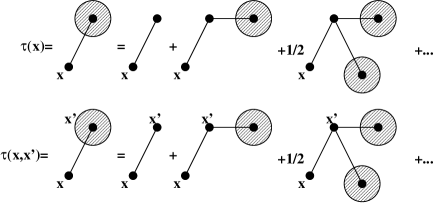
The function $\zeta[\tau({\rm\bf r})]$ represents the vertices at the point ${\rm\bf r}$ with an ${\rm\bf r}$-dependent weight $\tau({\rm\bf r})$ for each outgoing line. The latter represents the sum of all tree graphs starting at the position ${\rm\bf r}$. Its value is given by the implicit equation (218) which states that $\tau({\rm\bf r})$ equals the specific contribution of the first line $\xi({\rm\bf r},{\rm\bf r}^{\prime})$ multiplied by any kind of vertex $\nu_{q}$, the $q-1$ remaining lines being dressed by as many $\tau({\rm\bf r}^{\prime})$ factors. The sum over all possible vertices introduces the function ${{\rm d}\zeta\over{\rm d}\tau}[\tau({\rm\bf r}^{\prime})]$ (and not the function $\zeta[\tau({\rm\bf r}^{\prime})]$ since one line is treated apart) and an integration over ${\rm\bf r}^{\prime}$ is required to finally construct $\tau({\rm\bf r})$. The Fig. 10a presents a diagrammatic representation of the implicit equation (218).

An important remark that can already be made at this stage is that, although the matter particles outside the cell are strongly correlated with the ones inside, the generating function for the counts in a cell depends only on the correlations within this cell.

The next step is to simplify considerably the equations (216-218) by means of a “mean field” approximation that turned out to be extremely accurate (about $1$ to $2\%$, see discussion in BeS92). We integrate (218) over ${\rm\bf r}$ and then approximate $\tau({\rm\bf r})$ by a constant $\tau$. The equation (218) is then changed in,

$$\tau=(\lambda-1)\,n\,v\,\overline{\xi}\,{{\rm d}\zeta\over{\rm d}\tau}(\tau),$$ (219)

with

$$\overline{\xi}=\int_{v}{{\rm d}^{3}{\rm\bf r}\over v}\,{{\rm d}^{3}{\rm\bf r}^{\prime}\over v}\,\xi({\rm\bf r},{\rm\bf r}^{\prime}).$$ (220)

The equation (216) then reads,

$$\chi(\lambda)=(\lambda-1)\,n\,v\,\zeta(\tau)-{1\over 2}(\lambda-1)\,n\,v\,\tau{{\rm d}\zeta\over{\rm d}\tau}(\tau).$$ (221)

This is the form that is used for practical calculations.

In the limit of a continuous distribution, when $n$ goes to infinity for a given mass density $\rho$, the product $(1-\lambda)\,n$ remains finite. It will turn out to be convenient to define in this case the variable

$$y=(1-\lambda)\,n\,v\,\overline{\xi},$$ (222)

which remains finite. We are then led to use the function $\varphi(y)$ ,

$$\chi(\lambda)=-\varphi(y)/\overline{\xi},$$ (223)

and the relations (219-221) then read,

$$\varphi(y) = y\zeta(\tau)-{1\over 2}y\,\tau{{\rm d}\zeta\over{\rm d}\tau}(\tau)$$ (224)

$$\tau = -y{{\rm d}\zeta\over{\rm d}\tau}(\tau).$$ (225)

A.2 The general hierarchical model

So far we considered the minimal tree-hierarchical model, for which the coefficient $Q_{p}^{(\alpha)}$ are given by (214). In case of a general tree-hierarchical model, the equations (215-218) have to be modified to take into account the dependences of the coefficients $Q_{p}^{(\alpha)}$ with the geometry of the vertices,

$$Q_{p}^{(\alpha)}({\rm\bf r}_{1},\dots,{\rm\bf r}_{p})=\prod_{{\rm vertices}}\nu_{q}({\rm\bf r}_{s_{1}}-{\rm\bf r}_{i},\dots,{\rm\bf r}_{s_{q}}-{\rm\bf r}_{i}),$$ (226)

where the product is still over all the vertices associated with the tree topology $(\alpha)$, ${\rm\bf r}_{i}$ is the coordinate of the considered vertex and ${\rm\bf r}_{s_{1}},\dots,{\rm\bf r}_{s_{q}}$ are the coordinates of the end points of the $q$ outgoing lines of the vertex $n$. The difference with the previous calculation is that the vertex now depends on the geometry of the outgoing lines.

In this case we are led to define the function $\tau({\rm\bf r},{\rm\bf r}^{\prime})$ representing the sum of all tree graphs starting with the line that joins ${\rm\bf r}$ and ${\rm\bf r}^{\prime}$. The function $\tau({\rm\bf r})$ defined previously is simply the integral over ${\rm\bf r}^{\prime}$ of $\tau({\rm\bf r},{\rm\bf r}^{\prime})$ within the volume $v$.

The analogous of the equation (218) now reads (see also Fig. 10b)

$$\tau({\rm\bf r},{\rm\bf r}^{\prime})=(\lambda-1)\,n\,\xi({\rm\bf r},{\rm\bf r}^{\prime})$$ (227)

$$\ \times\left[1+\sum_{q=2}^{\infty}\int_{v}{\rm d}^{3}{\rm\bf r}_{1}\dots{\rm d}^{3}{\rm\bf r}_{q-1}{(-1)^{q-1}\over(q-1)!}\right.$$

$$\ \times\left.\,\nu_{q}({\rm\bf r}^{\prime}\!-\!{\rm\bf r},{\rm\bf r}^{\prime}\!-\!{\rm\bf r}_{1},\dots,{\rm\bf r}^{\prime}\!-\!{\rm\bf r}_{q-1})\,\tau({\rm\bf r}^{\prime},{\rm\bf r}_{1})\dots\tau({\rm\bf r}^{\prime},{\rm\bf r}_{q-1})\right].$$

It can be easily checked that this equation gives (218) when the vertices are pure numbers by an integration over ${\rm\bf r}^{\prime}$. The function $\chi(\lambda)$ is now given by ($\nu_{1}\equiv 1$),

$$\chi(\lambda)=\int_{v}(\lambda-1)\,n\,{\rm d}^{3}{\rm\bf r}$$

$$\ \ \ +\sum_{q=1}^{\infty}(1-{q\over 2})\int_{v}(\lambda-1)\,n\,{\rm d}^{3}{\rm\bf r}\,{\rm d}^{3}{\rm\bf r}_{1}\dots{\rm d}^{3}{\rm\bf r}_{q}{(-1)^{q}\over q!}\times$$

$$\ \ \,\times\nu_{q}({\rm\bf r}-{\rm\bf r}_{1},\dots,{\rm\bf r}-{\rm\bf r}_{p})\,\tau({\rm\bf r},{\rm\bf r}_{1})\dots\tau({\rm\bf r},{\rm\bf r}_{q}),$$ (228)

which also reduces to (216) in case of the minimal model. In the general case there is still a possible “mean field” approximation which just assumes that $\tau({\rm\bf r},{\rm\bf r}^{\prime})$ is proportional to $\xi({\rm\bf r},{\rm\bf r}^{\prime})$,

$$\tau({\rm\bf r},{\rm\bf r}^{\prime})\approx{\tau\over\overline{\xi}}\,\xi({\rm\bf r},{\rm\bf r}^{\prime}).$$ (229)

We are then led to exactly the same equation (219-225) for $\chi(\lambda)$ and $\varphi(y)$ with $\zeta(\tau)$ given by (215) and the vertices $\nu_{q}$ defined by the expectation values

$$\nu_{q}=\int_{v}{{\rm d}^{3}{\rm\bf r}\over v}\,\nu_{q}({\rm\bf r}-{\rm\bf r}_{1},\dots,{\rm\bf r}-{\rm\bf r}_{q})\prod_{i=1}^{q}{\xi({\rm\bf r},{\rm\bf r}_{i})\over\overline{\xi}}\,{{\rm d}^{3}{\rm\bf r}_{i}\over v}.$$ (230)

Obviously, the validity of such an approximation depends on the strength of the geometrical dependences of $\nu_{q}({\rm\bf r}-{\rm\bf r}_{1},\dots,{\rm\bf r}-{\rm\bf r}_{q})$. We assume here that they are weak enough so that the mean field approximation is valid.

A.3 The calculation of $p(N)$

In the limit of a continuous distribution of matter we have the relations

$$e^{-{\varphi(y)\over\overline{\xi}}} = \int_{0}^{\infty}{\rm d}m\ e^{-{m\over m_{{\rm c}}}y}\,p(m)\,$$ (231)

$$p(m)\,{\rm d}m = \displaystyle{{{\rm d}m\over m_{{\rm c}}}\,\int_{-{\rm i}\infty}^{+{\rm i}\infty}{{\rm d}y\over 2\pi{\rm i}\,}\,e^{-{\varphi(y)\over\overline{\xi}}+{m\over m_{{\rm c}}}y}},$$ (232)

with,

$$m_{{\rm c}}=\overline{m}\,\overline{\xi},\ \ \ \overline{m}=\rho\,v,,$$ (233)

where $\overline{m}$ is the mean mass contained in a cell of volume $v$. The counts in cells are then obtained by a simple Poisson convolution of Eq. (232).

Realistic models for $p(N)$ and hence $\varphi(y)$ or $\zeta(\tau)$ have been widely discussed (Schaeffer 1985, BaS89, BeS92). Generically $\varphi(y)$ must have singularities at negative $y$ and behave as $y^{(1-\omega)}$ at large $y$, with $0\leq\omega\leq 1$. In the strongly non-linear regime $\overline{\xi}\gg 1$, (232) can be simplified into,

$$p(m)\,{\rm d}m=\displaystyle{-{{\rm d}m\over m_{{\rm c}}\overline{\xi}}\,\int_{-{\rm i}\infty}^{+{\rm i}\infty}{{\rm d}y\over 2\pi{\rm i}}\,\varphi(y)e^{{m\over m_{{\rm c}}}}y}.$$ (234)

This form holds provided ${\varphi(y)/\overline{\xi}}$ is small. For low values of $m$, however, $y\propto{m_{{\rm c}}/m}$ gets large and,

$${\varphi(y)\over\overline{\xi}}\propto({m_{{\rm c}}\over m})^{(1-\omega)}/\overline{\xi},$$ (235)

may not be small enough. The form (234) thus holds only provided,

$$m\gg m_{{\rm v}}=m_{{\rm c}}/\overline{\xi}^{1\over 1-\omega}.$$ (236)

The halos referred to in this paper are those for which (236) is satisfied.

Appendix B Joint counts in cells

We use the same partition of the universe into cells of volume $v_{i}$ (which are not necessarily the same) as in the Appendix A and consider a set of ${\cal N}$ cells denoted by the index $i=1\dots{\cal N}$. We aim to calculate the probability that $N_{1}$ elementary objects are in cell 1 at position ${\rm\bf r}_{1}$, $N_{2}$ in cell 2 at position ${\rm\bf r}_{2}$, … The corresponding generating function is,

$$e^{\chi(\lambda_{1},\dots,\lambda_{{\cal N}})}=$$

$$\ \ \ \sum_{N_{1}}\dots\sum_{N_{{\cal N}}}\ \left(\prod_{i=1}^{{\cal N}}\lambda_{i}^{N_{i}}\right)\ p(N_{1},\dots,N_{{\cal N}}).$$ (237)

In case $\chi(\lambda_{1},\dots,\lambda_{{\cal N}})$ is known, $p(N_{1},\dots,N_{{\cal N}})$ can be obtained through,

$$p(N_{1},\dots,N_{{\cal N}})={1\over(2\pi{\rm i})^{{\cal N}}}\ \oint\prod_{i=1}^{{\cal N}}\ {{\rm d}\lambda_{i}\over\lambda_{i}^{N_{i}+1}}\times$$

$$\ \ \ \times e^{\chi(\lambda_{1},\dots,\lambda_{{\cal N}})}.$$ (238)

We may ask for the probability that cells $1,\dots,P$, which are assumed to all lie with a larger finite volume $V$, contain respectively $N_{1},\dots,N_{P}$ elementary particles, whatever the contents of the cells $P+1$ to ${\cal N}$ are. This amounts to sum over $N_{P+1},\dots,N_{{\cal N}}$ in (237) with $\lambda_{P+1},\dots,\lambda_{{\cal N}}$ all equal to unity. It is important to note that in this case all integrations over the variables within cells $P+1$ to ${\cal N}$ drop out: the sums simply run from $i=1$ to $P$. In case $P=1$ we simply recover the expressions (209, 210) for the counts in one cell, the solution of which is given by the equations (219-225).

From now on we will always implicitly assume that the cells $1,\dots,P$ all lie within a volume $V$, much larger than the volume $v_{i}$ ( $v_{i}\ll V$) of the elementary cells.

B.1 General properties of the generating function $\chi$

B.1.1 The minimal tree-hierarchical model

Once again the minimal tree-hierarchical model is simpler and deserves to be treated separately. The function $\chi$ can be constructed in a similar way than in (216, 218). The only change is that the value of $\lambda$ depends on the volume in which the corresponding point lies.

The equation for $\tau({\rm\bf r})$ now reads,

$$\tau({\rm\bf r})=\sum_{i=1}^{P}\ \int_{v_{i}}(\lambda_{i}-1)\ n\ {\rm d}^{3}{\rm\bf r}^{\prime}\xi({\rm\bf r},{\rm\bf r}^{\prime}){{\rm d}\zeta\over{\rm d}\tau}[\tau({\rm\bf r}^{\prime})].$$ (239)

and the expression of $\chi$ is,

$$\chi(\lambda_{1},\dots,\lambda_{P})=\sum_{i=1}^{P}\,\int_{v_{i}}(\lambda_{i}-1)\,n\,{\rm d}^{3}{\rm\bf r}\,\zeta[\tau({\rm\bf r})]\,$$

$$\ \ \ \displaystyle{-{1\over 2}\sum_{i=1}^{P}\,\int_{v_{i}}(\lambda_{i}-1)\,n\,{\rm d}^{3}{\rm\bf r}\,\tau({\rm\bf r}){{\rm d}\zeta\over{\rm d}\tau}[\tau({\rm\bf r})]}.$$ (240)

Once again we can introduce a mean field approximation. We assume that $\tau({\rm\bf r})$ has a constant value $t_{i}$ within each volume $i$. The equation for $t_{i}$ can be obtained from (239),

$$t_{i}=(\lambda_{i}-1)\,n\,v_{i}\,\overline{\xi}_{i}\,{{\rm d}\zeta\over{\rm d}\tau}(t_{i})+\sum_{j\neq i}(\lambda_{j}\!-\!1)\,n\,v_{j}\,\overline{\xi}_{ij}\,{{\rm d}\zeta\over{\rm d}\tau}(t_{j})$$ (241)

where $\overline{\xi}_{i}$ is the mean value of $\xi({\rm\bf r},{\rm\bf r}^{\prime})$ within the volume $i$ and $\overline{\xi}_{ij}$ is its means value when ${\rm\bf r}$ is in $v_{i}$ and ${\rm\bf r}^{\prime}$ in $v_{j}$.

For convenience, we split $t_{i}$ into two terms $\tau_{i}$ and $\theta_{i}$,

$$\tau_{i} = (\lambda_{i}-1)\,n\,v_{i}\,\overline{\xi}_{i}\,{{\rm d}\zeta\over{\rm d}\tau}(\tau_{i}+\theta_{i}),$$ (242)

$$\theta_{i} = \sum_{j\neq i}(\lambda_{j}-1)\,n\,v_{j}\,\overline{\xi}_{ij}\,{{\rm d}\zeta\over{\rm d}\tau}(\tau_{j}+\theta_{j}).$$ (243)

The notation $\tau_{i}$ corresponds to graphs the first line of which starts and ends within the same box $i$, whereas $\theta_{i}$ corresponds to graphs that start in the box $i$ but immediately join another box $j\neq i$. The function $\chi(\lambda_{1},\dots,\lambda_{P})$ is now given by,

$$\chi(\lambda_{1},\dots,\lambda_{P})=\sum_{i=1}^{P}\,(\lambda_{i}-1)\,n\,v_{i}\,\zeta(\tau_{i}+\theta_{i})$$

$$\ \ \ -{1\over 2}\sum_{i=1}^{P}(\lambda_{i}-1)\,n\,v_{i}\,(\tau_{i}+\theta_{i}){{\rm d}\zeta\over{\rm d}\tau}(\tau_{i}+\theta_{i}).$$ (244)

The same summation can be written in a different way that will turn out to be useful in the following. We can first focus on one cell. Let us define $\chi(\lambda,\theta)$ by,

$$\chi(\lambda,\theta)=(\lambda-1)\,n\,v\,\zeta[\tau(\lambda,\theta)+\theta]$$

$$\ \ \ -{1\over 2}(\lambda-1)\,n\,v\,\tau(\lambda,\theta){{\rm d}\zeta\over{\rm d}\tau}[\tau(\lambda,\theta)+\theta],$$ (245)

with,

$$\tau(\lambda,\theta)=(\lambda-1)\,n\,v\,\overline{\xi}(v)\,{{\rm d}\zeta\over{\rm d}\tau}(\tau(\lambda,\theta)+\theta).$$ (246)

These relations define $\chi(\lambda,\theta)$ as a function of two variables $\lambda$ and $\theta$ (and the volume of the cell $v$). This function is the sum off all connected tree graphs within the cell (with vertices only in the cell, all being connected by lines) having an arbitrary number of outgoing lines, each weighted by a factor $\theta$. The generating function $\chi(\lambda_{1},\dots,\lambda_{P})$ can be built up with the functions $\chi(\lambda_{i},\theta),i=1,\dots,P$ once $\theta$ is specified for each values of $i$. The basic property required for such a construction is that one can relate the partial derivative of $\chi(\lambda,\theta)$ relatively to $\theta$ (for a fixed $\lambda$) to the derivative of $\zeta$,

$$\left.{\partial\chi\over\partial\theta}\right.(\lambda,\theta)=(\lambda-1)\,n\,v\,{{\rm d}\zeta\over{\rm d}\tau}(\tau(\lambda,\theta)+\theta)$$ (247)

with $\tau(\lambda,\theta)$ given by (246).

As a result the equation (243) can be written using the function $\chi(\lambda,\theta)$ instead of the function $\zeta$,

$$\theta_{i}=\sum_{j\neq i}\overline{\xi}_{ij}\,\left.{\partial\chi\over\partial\theta}\right.(\lambda_{j},\theta_{j}),$$ (248)

and the function $\chi(\lambda_{1},\dots,\lambda_{P})$ now reads

$$\chi(\lambda_{1},\dots,\lambda_{P})=\sum_{i=1}^{P}\chi(\lambda_{i},\theta_{i})-{1\over 2}\sum_{i=1}^{P}\theta_{i}{\partial\chi\over\partial\theta}(\lambda_{i},\theta_{i}).$$ (249)

The equations (248) and (249) are similar to the equations (219-225), where $\zeta(\tau)$ has been replaced by $\chi(\lambda,\theta)$ as a function of $\theta$ and where the matter have been replaced by cells of weight $(\lambda_{i}-1)\,n\,v_{i}$. The function $\chi(\lambda,\theta)$ is the sum of all diagrams within a given cell when the environment of the cell has a weight $\theta$. The function $\chi(\lambda)$ in the appendix A corresponds to the case when no constraints have been put in the vicinity of the cell $i$, that is given by $\theta=0$, so that $\chi(\lambda)=\chi(\lambda,\theta=0)$.

The form $\chi(\lambda,\theta)$ is the central relation for the construction of the statistics of the content of a large cell $V$ in terms of the elementary finite cells $v_{i}$, instead of the elementary points of matter as in the Appendix A. That will be the ground for joint count-in-cell calculations.

B.1.2 The general tree-hierarchical model

The case of the general tree-hierarchical models is basically the same although technically more complicated.

The equation for $\tau({\rm\bf r},{\rm\bf r}^{\prime})$ now reads when ${\rm\bf r}^{\prime}$ is in the cell $j$,

$$\tau({\rm\bf r},{\rm\bf r}^{\prime})=(\lambda_{j}-1)\,n\,\xi({\rm\bf r},{\rm\bf r}^{\prime})\left[1+\sum_{q=2}^{\infty}\sum_{i_{1}=1}^{P}\dots\sum_{i_{q-1}=1}^{P}\right.$$

$$\ \ \ \left.\times\int_{v_{i_{1}}}{\rm d}^{3}{\rm\bf r}_{1}\dots\int_{v_{i_{q-1}}}{\rm d}^{3}{\rm\bf r}_{q-1}\nu_{q}({\rm\bf r}^{\prime}\!-\!{\rm\bf r},{\rm\bf r}^{\prime}\!-\!{\rm\bf r}_{1},\dots,{\rm\bf r}^{\prime}\!-\!{\rm\bf r}_{q-1})\right.$$

$$\ \ \ \left.\times{(-1)^{q-1}\over(q-1)!}\,\tau({\rm\bf r}^{\prime},{\rm\bf r}_{1})\dots\tau({\rm\bf r}^{\prime},{\rm\bf r}_{q-1})\right].$$ (250)

The expression of $\chi$ has to be changed in a similar way,

$$\chi(\lambda_{1},\dots,\lambda_{P})=\sum_{i=1}^{P}\int_{v_{i}}(\lambda_{i}-1)\,n{\rm d}^{3}{\rm\bf r}+\sum_{q=1}^{\infty}(1-{q\over 2})$$

$$\ \ \ \times\sum_{i=1}^{P}\sum_{i_{1}=1}^{P}\dots\!\sum_{i_{q}=1}^{P}\int_{v_{i}}(\lambda_{i}\!-\!1)n{\rm d}^{3}{\rm\bf r}\int_{v_{i_{1}}}{\rm d}^{3}{\rm\bf r}_{1}\dots\int_{v_{i_{q}}}{\rm d}^{3}{\rm\bf r}_{q\!-\!1}$$

$$\ \ \ \times{(-1)^{q}\over q!}\nu_{q}({\rm\bf r}-{\rm\bf r}_{1},\dots,{\rm\bf r}-{\rm\bf r}_{q})\,\tau({\rm\bf r},{\rm\bf r}_{1})\dots\tau({\rm\bf r},{\rm\bf r}_{q}).$$ (251)

The extension of the mean field approximation leads to assume that,

$$\tau({\rm\bf r},{\rm\bf r}^{\prime})\approx\tau_{ij}{\xi({\rm\bf r},{\rm\bf r}^{\prime})\over\overline{\xi}_{ij}}$$ (252)

where ${\rm\bf r}$ is in the volume $i$ and ${\rm\bf r}^{\prime}$ in the volume $j$. The value of $\tau_{i}$ corresponding to the definition (242) is,

$$\tau_{i}=\int_{v_{i}}{{\rm d}^{3}{\rm\bf r}\over v_{i}}\,\int_{v_{i}}{{\rm d}^{3}{\rm\bf r}^{\prime}\over v_{i}}\tau({\rm\bf r},{\rm\bf r}^{\prime})=\tau_{ii},$$ (253)

whereas,

$$\theta_{i}=\int_{v_{i}}{{\rm d}^{3}{\rm\bf r}\over v_{i}}\,\sum_{j\neq i}\int_{v_{j}}{{\rm d}^{3}{\rm\bf r}^{\prime}\over v_{j}}\tau({\rm\bf r},{\rm\bf r}^{\prime})=\sum_{j\neq i}\tau_{ij}.$$ (254)

Our aim is to calculate (251) with the mean field approximation. The quantities $\tau_{ij}$ in fact depend not only on $\lambda_{1},\dots,\lambda_{P}$ but also on the positions of the cells in the volume $V$. In case of the minimal tree-hierarchical model this dependence is completely determined by the values of $\overline{\xi}_{ij}$. For the general case the vertices introduce some extra geometrical dependences. We then are led to introduce a second mean field approximation which is to assume that $\tau_{ij}$ is just proportional to $\overline{\xi}_{ij}$ as far as the positions of the cells are considered. It just leads to change the equation (252) in,

$$\tau({\rm\bf r},{\rm\bf r}^{\prime})=\tau_{i}{\xi({\rm\bf r},{\rm\bf r}^{\prime})\over\overline{\xi}_{i}},$$ (255)

when ${\rm\bf r}$ and ${\rm\bf r}^{\prime}$ are in $v_{i}$ and,

$$\tau({\rm\bf r},{\rm\bf r}^{\prime})=\tau_{ij}{\xi({\rm\bf r},{\rm\bf r}^{\prime})\over\overline{\xi}(V)},$$ (256)

when ${\rm\bf r}$ and ${\rm\bf r}^{\prime}$ are in two different cells $v_{i}$ and $v_{j}$. $\overline{\xi}(V)$ is the mean value of the two-point matter correlation function in the large volume $V$. The transformation of the relation (250) and (251) introduces the geometrical averages,

$$\nu_{q,Q}=$$

$$\ \ \ \int_{V}{{\rm d}^{3}{\rm\bf r}\over V}{{\rm d}^{3}{\rm\bf r}_{1}\over V}\dots{{\rm d}^{3}{\rm\bf r}_{Q}\over V}\int_{v}{{\rm d}^{3}{\rm\bf r}_{Q+1}\over v}\dots{{\rm d}^{3}{\rm\bf r}_{q}\over v}$$

$$\ \ \ \times\nu_{q}({\rm\bf r}_{1}-{\rm\bf r},\dots,{\rm\bf r}_{Q}-{\rm\bf r},{\rm\bf r}_{Q+1}-{\rm\bf r},\dots,{\rm\bf r}_{q}-{\rm\bf r})$$

$$\ \ \ \times{\xi({\rm\bf r}_{1},{\rm\bf r})\over\overline{\xi}(V)}\dots{\xi({\rm\bf r}_{Q},{\rm\bf r})\over\overline{\xi}(V)}{\xi({\rm\bf r}_{Q+1},{\rm\bf r})\over\overline{\xi}(v)}\dots{\xi({\rm\bf r}_{q},{\rm\bf r})\over\overline{\xi}(v)}.$$ (257)

The index $q$ is the total number of lines and $Q$ is the number of long lines (going from one cell to another). As soon as $v\ll V$, the averages $\nu_{q,Q}$ are independent of the partition of $V$ in small cells. These generalized vertices are thus specific of the matter correlation properties.

We then define the generating function $\zeta(\tau,\theta)$ of this vertices

$$\zeta(\tau,\theta)=\sum_{q,Q}\,\nu_{q,Q}{(-1)^{q-Q}\tau^{q-Q}\over(q-Q)!}{(-1)^{Q}\theta^{Q}\over Q!}.$$ (258)

For the minimal tree-hierarchical model we simply have

$$\zeta(\tau,\theta)=\zeta(\tau+\theta).$$ (259)

The equation for $\tau_{i}$ and $\theta_{i}$ now reads

$$\tau_{i} = (\lambda_{i}-1)\,n\,v_{i}\,\overline{\xi}_{i}\,{\partial\zeta\over\partial\tau}(\tau_{i},\theta_{i});$$ (260)

$$\theta_{i} = \sum_{j\neq i}(\lambda_{j}-1)\,n\,v_{j}\,\overline{\xi}(V)\,{\partial\zeta\over\partial\theta}(\tau_{j},\theta_{j})$$ (261)

and

$$\chi(\lambda_{1},\dots,\lambda_{P})=\sum_{i=1}^{P}\,(\lambda_{i}-1)\,n\,v_{i}\,\zeta(\tau_{i},\theta_{i})$$

$$\ \ \ -{1\over 2}\sum_{i=1}^{P}(\lambda_{i}-1)\,n\,v_{i}\,\tau_{i}{\partial\zeta\over\partial\tau}(\tau_{i},\theta_{i})$$

$$\ \ \ -{1\over 2}\sum_{i=1}^{P}(\lambda_{i}-1)\,n\,v_{i}\,\theta_{i}{\partial\zeta\over\partial\theta}(\tau_{i},\theta_{i}).$$ (262)

The expression of $\chi(\lambda_{1},\dots,\lambda_{P})$ can be transformed as previously in a tree-graph summation. We define $\chi(\lambda,\theta)$ by

$$\chi(\lambda,\theta)=(\lambda-1)\,n\,v\,\zeta[\tau(\lambda,\theta),\theta]$$

$$\ \ \ -{1\over 2}(\lambda-1)\,n\,v\,\tau(\lambda,\theta){\partial\zeta\over\partial\tau}[\tau(\lambda,\theta),\theta]$$ (263)

with

$$\tau(\lambda,\theta)=(\lambda-1)\,n\,v\,\overline{\xi}(v)\,{\partial\zeta\over\partial\tau}[\tau(\lambda,\theta),\theta].$$ (264)

We get an equation similar to (247),

$${\partial\chi\over\partial\theta}(\lambda,\theta)=(\lambda-1)\,n\,v\,{\partial\zeta\over\partial\theta}(\tau,\theta)$$ (265)

and the function $\chi(\lambda_{1},\dots,\lambda_{P})$ is the same than in (248, 249):

$$\theta_{i} = \sum_{j\neq i}\overline{\xi}(V)\,{\partial\chi\over\partial\theta}(\lambda_{j},\theta_{j})$$ (266)

$$\chi(\lambda_{1},\dots,\lambda_{P}) = \sum_{i=1}^{P}\chi(\lambda_{i},\theta_{i})-{1\over 2}\sum_{i=1}^{P}\theta_{i}{\partial\chi\over\partial\theta}(\lambda_{i},\theta_{i}).$$ (267)

The only difference between the minimal tree model and the general case is that in the latter we are led, in order to get tractable calculations, to integrate out the position dependence of the $P$ cells, and thus replace $\overline{\xi}_{ij}$ in (248) by $\overline{\xi}(V)$. The information we get from the spatial dependences of the halo correlation functions is then poorer in this case. Nevertheless, for a very large variety of applications (see Schaeffer 1984, 1985, 1987, and the extended discussion in BeS92) we can accurately use the averages of these correlation functions in the volume $V$, as it is shown in the next appendix.

B.1.3 Diagrammatic representations

The equations (249) and (267) are decisive results for joint counts in cells calculations. They deserve attention. The function $\chi(\lambda_{1},\dots,\lambda_{P})$ is the sum of all connected tree graphs with their proper weights, as explained in the beginning of this section. These relations mean that such a summation can be performed in two steps. Indeed one can first compute the sum of all graphs having their vertices in a given cell and a given number, say $Q$, of outgoing lines (Fig 11). Let us denote $\chi_{Q}(\lambda)$ such a sum. The generating function for these graphs is precisely the function $\chi(\lambda,\theta)$ (Eqs. [245] and [263]) calculated in the given cell, $\theta$ being the weight attached to each free line. The expansion of $\chi(\lambda,\theta)$ in powers of $\theta$,

$$\chi(\lambda,\theta)=\sum_{Q}(-1)^{Q}\chi_{Q}(\lambda){\theta^{Q}\over Q!}$$ (268)

then leads to the corresponding sums $\chi_{Q}(\lambda)$. Once the sum within an elementary cell is known, $\chi(\lambda_{1},\dots,\lambda_{P})$ is obtained by connecting (Fig. 12) the different cells in all possible ways, each connection between, say cell $i$ and $j$, having a weight $\overline{\xi}_{ij}$ for the case of the minimal tree model, or simply $\overline{\xi}(V)$ for the general case. These connections build a new tree whose elementary vertices are the graphs already summed within one cell.

Figure 11: Example of a contribution to the function $\chi_{3}(\lambda)$. This is the sum of all the trees within a given box with three external lines. These lines each have the weight $\theta$.

Figure 12: Decomposition of the sum $\chi(\lambda_{1},\dots,\lambda_{I})$ in product of functions $\chi_{Q}(\lambda_{i})$. The term that appears in the figure involves 4 cells with the product $\chi_{1}(\lambda_{1})\allowbreak\xi_{12}\allowbreak\chi_{3}(\lambda_{2})\allowbreak\xi_{2j_{1}}\allowbreak\xi_{23}\allowbreak\chi_{3}(\lambda_{3})\allowbreak\xi_{3j_{2}}\allowbreak\xi_{34}\allowbreak\chi_{3}(\lambda_{4})\allowbreak\xi_{4j_{3}}\allowbreak\xi_{4j_{4}}\dots.$ The external lines are connected to other cells of the volume $V$ (with the indices $j_{1}$,$j_{2}$, $j_{3}$ and $j_{4}$)

At this point however loops between cells are not excluded. They arise when a cell is reached again after having been connected to various neighboring cells. It can be seen in Fig. 13a that the original graph, at the matter point level, has no loops according to the rules of the general hierarchical model although the graph at the cell level contains one loop.

B.2 Correlations among cells

Figure 13: Two examples of contribution to the sum $\chi(\lambda_{1},\lambda_{2},\lambda_{3})$ that make intervene the same number of points in each of the cells. The first one (a) creates a loop between the cells although it is a tree at the matter point level. The second one (b) is a tree even at the cells level. The ratio between these two contributions is of the order of $\xi_{13}/\overline{\xi}(v)$ (where $\overline{\xi}(v)$ is the mean value of the two-point matter correlation function in the volume $v$ of a cell). In most of the relevant cases the contributions with loops will then be negligible compare to the trees.

B.2.1 General expression

From the expression of the generating function $\chi(\lambda_{1},\dots,\lambda_{P})$ of the connected graph we now seek for the probability $p(N_{1},{\rm\bf r}_{1};\dots;N_{P},{\rm\bf r}_{P})$ using the general formula (238). An explicit calculation is possible when one assumes that the distances between the cells are large compare to their size so that we have,

$$\overline{\xi}_{ij}\ll\overline{\xi}(v).$$ (269)

Let us first inspect the structure of $\chi(\lambda_{1},\dots,\lambda_{P})$ with the assumption (269), having in mind we seek a perturbation expansion in $\xi_{ij}/\overline{\xi}(v)$. The function $\chi(\lambda_{1},\dots,\lambda_{P})$ is a sum of tree graphs (Fig.13) connecting points within the various cell $i=1,\ldots,P$, each connection being weighted by the average $\overline{\xi}(v_{i})$ of the correlation function within the cell, and points belonging to two different cells, say $i$ and $j$, with a weight $\xi_{ij}$. That this is the case in general is readily seen from equation (268) where the weight of an external line appears indeed to be proportional to $\xi_{ij}$ whereas an internal line has the weight $\overline{\xi}$. The condition (269) insures that a graph that contains a loop (that is coming back to a given cell after having visited other cells) introduces a factor $\xi_{ij}/\overline{\xi}\ll 1$ more than the same graph (same number of points in each of the cells) (Fig. 13b) that does not contain the loop. In the limit (269), at leadind order, the remaining contribution to $\chi(\lambda_{1},\dots,\lambda_{P})$ is the sum with the smallest number of external lines connecting the different cells. Whence, in the limit (269), each cell appears only once in each remaining graphs. Each cell (as in Fig. 12) then appear as a dressed point (see Fig. 11) with outgoing lines that connect this cell to other ones.

The sum of the remaining graphs is then a sum of product of factors $\chi_{Q}(\lambda)$ corresponding to different cells:

$$\chi(\lambda_{1},\dots,\lambda_{P})=\sum_{{\rm tree\ graphs}}\,C_{{Q}_{1},\dots,{Q}_{P}}$$

$$\ \ \ \times\chi_{{Q}_{1}}(\lambda_{1})\dots\chi_{{Q}_{P}}(\lambda_{P}),$$ (270)

where $C_{{Q}_{1},\dots,{Q}_{P}}$ is independent of the parameters $\lambda$.

Figure 14: Two examples of contribution to $p(N_{1},N_{2},N_{3})$ that appear when $\exp[\chi(\lambda_{1},\lambda_{2},\lambda_{3})]$ is expanded. The first diagram is negligible compared to a diagram where a $\xi_{ij}$ factor has been replaced by a $\overline{\xi}$ factor that still connect the three boxes. The second diagram cannot be a priori neglected : if a $\xi_{ij}$ factor is replaced by a $\overline{\xi}$ factor the three cells are not connected anymore.

This, however is true for $\chi(\lambda_{1},\dots,\lambda_{P})$ whereas (238) involves $\exp[\chi(\lambda_{1},\dots,\lambda_{P})]$. We therefore should extend the above examination to the latter. While the former is the sum of all connected tree graphs, the latter is the sum of all, connected or disconnected, tree graphs where now the contribution of graphs in which all points are not linked together is also included (the same way that the generating function of the cumulants is given by the logarithm of the generating function of the moments).

From Fig. 14a it is clear the expansion of $\exp[\chi(\lambda_{1},\dots,\lambda_{P})]$ into tree graphs, not only brings in additional disconnected graphs but also, as previously, loops between boxes. We now proceed by selecting the connected contributions at the cell level, that is by identifying those graphs in which all cells are connected together (but with possible disconnected parts within the cells). These contributions may thus be built from disconnected diagrams at the matter level, that become connected at the cell level. However for the same reason as for Fig. 13a, diagrams similar to Fig. 14a that build up loops among the cells have a negligible contribution : it is always possible to change a $\xi_{ij}$ factor by a $\overline{\xi}$ factor and to preserve the connection between the boxes. This is not the case for diagrams like in Fig. 14b : in such a case changing a $\xi_{ij}$ factor by a $\overline{\xi}$ factor breaks the connection between the cells. It is therefore not possible a priori to neglect the latter contributions.

Eventually we then are left with diagrams that form trees between cells in which the “dressed” vertices of order $Q$ corresponding to each cell are obtained by the summation of all diagrams - connected or not within the cell- having $Q$ outgoing lines.

We know that the generating function of the connected diagrams in a cell, with outgoing lines weighted by $\theta$, is $\chi(\lambda,\theta)$. The generating function of all diagrams, connected or unconnected, is therefore $\exp[\chi(\lambda,\theta)]$ . This point can be illustrated for the diagrams with one external line (e.g. on Fig. 15). The connected diagrams with one external line are given by $\chi_{1}(\lambda)$. Adding diagrams with no external lines amounts to multiply $\chi_{1}(\lambda)$ by the generating function of those diagrams, $\exp[\chi(\lambda)]$ and the fist derivative of $\exp[\chi(\lambda,\theta)]$ with respect to $\theta$ is indeed $\chi_{1}(\lambda)\,\exp[\chi(\lambda)]$.

Figure 15: Contruction of the generating function of $b(N)p(N)$. It involves all possible diagrams, connected or not, that have one external line. It can be built from the generating function of the connected diagrams with one external line, $\chi_{1}$, and the generating function of the diagrams with no external lines, $\chi$.

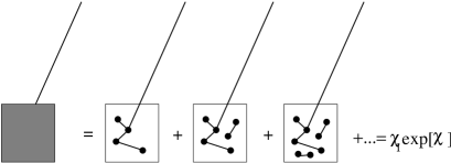
In a similar way than at the end of the appendix A, we may introduce the function $\varphi(y,\theta)$ defined by,

$$\chi(\lambda,\theta)=-\varphi(y,\theta)/\overline{\xi}(v),$$ (271)

that changes the equation (263, 264) in

$$\varphi(y,\theta) = y\zeta(\tau,\theta)-{1\over 2}y\,\tau{\partial\zeta\over\partial\tau}(\tau,\theta)$$ (272)

$$\tau = -y\,{\partial\zeta\over\partial\tau}(\tau,\theta)$$ (273)

$y$ being defined in (222). Then in case we are only interested in large values of $N$, in such a way that,

$$N\gg N_{{\rm v}}=n\,v\,\overline{\xi}^{-\omega/(1-\omega)},$$ (274)

then $\chi(\lambda,\theta)$ is of the order of $1/\overline{\xi}$ ($y$ is finite in Eq. 271, see the discussion at the end of A for the case where (274) is not fulfilled). So, $\exp[\chi(\lambda,\theta)]\approx 1+\chi(\lambda,\theta)$ so that only connected diagrams contribute to the dressed vertices. This is also the result we could have obtained directly by writing $\exp[\chi(\lambda_{1},\ldots,\lambda_{P})]\sim 1+\chi(\lambda_{1},\ldots,\lambda_{P})$ , as can be inferred from the discussion at the beginning of this paragraph.

In all cases, whether $N$ is larger than $N_{{\rm v}}$ or not, each cell appears only once in each term of the expansion of $\exp[\chi(\lambda_{1},\ldots,\lambda_{P})]$ : at the cell level all diagrams are connected trees. The integration (238) over $\lambda_{1},\dots,\lambda_{P}$ is thus easily performed, and amounts to replace each factor depending only on the variable $\lambda_{i}$ of one specific cell by its integral ${1/(2\pi{\rm i})}\allowbreak\times\int{\rm d}\lambda_{i}/\lambda_{i}^{N_{i}+1}$. This simply amounts to replace the sum in a given cell of all graphs with external lines $\exp[\chi(\lambda,\theta)]$ by,

$$p(N,\theta)={1\over 2\pi{\rm i}}\int{{\rm d}\lambda\over\lambda^{N+1}}e^{\chi(\lambda,\theta)}$$ (275)

and to use these new generating functions as elementary vertices. For dense cells (with the meaning of Eq. [274]) this expression can be simplified as

$$p(N,\theta)={1\over 2\pi{\rm i}}\int{{\rm d}\lambda\over\lambda^{N+1}}\chi(\lambda,\theta).$$ (276)

As for the matter distribution (Eq. [215]), we can define the generating function of the vertices $\zeta(N,\theta)$ (App. A) by,

$$p(N,\theta)=p(N)\,\zeta(N,\theta)$$ (277)

recalling that $p(N)\equiv p(N,0)$. The expansion of $\zeta(N,\theta)$ in powers of $\theta$ defines new vertices $\nu_{Q}(N)$,

$$\zeta(N,\theta)=\sum_{Q}(-1)^{Q}\nu_{Q}(N)\,{\theta^{Q}\over Q!},$$ (278)

that replace the parameter $\nu_{q}$ relevant for the matter distribution. We have, for instance

$$\nu_{1}(N)p(N) \equiv b(N)p(N)$$ (279)

$$= -{1\over 2\pi{\rm i}}\int{{\rm d}\lambda\over\lambda^{N+1}}\chi_{1}(\lambda)e^{\chi(\lambda)};$$

$$\nu_{2}(N)p(N) = {1\over 2\pi{\rm i}}\int{{\rm d}\lambda\over\lambda^{N+1}}\left[\chi_{2}(\lambda)+\chi_{1}^{2}(\lambda)\right]\,e^{\chi(\lambda)}.$$ (280)

In the continuous limit we can further make the change of variable $\lambda\to y$ (e.g. Eq. 224) and we have,

$$b(m)p(m) = {1\over m_{{\rm c}}}\int_{-{\rm i}\infty}^{+{\rm i}\infty}{{\rm d}y\over 2\pi{\rm i}}{\varphi^{(1)}(y)\over\overline{\xi}}$$ (281)

$$\times\ e^{-{\varphi(y)/\overline{\xi}}+y\,{m/m_{{\rm c}}}};$$

$$\nu_{2}(m)p(m) = -{1\over m_{{\rm c}}}\int_{-{\rm i}\infty}^{+{\rm i}\infty}{{\rm d}y\over 2\pi{\rm i}}\left[{\varphi^{(2)}(y)\over\overline{\xi}}-\left(\varphi^{(1)}(y)\over\overline{\xi}\right)^{2}\right]\$$ (282)

$$\times\ e^{-{\varphi(y)/\overline{\xi}}+y\,{m/m_{{\rm c}}}},$$

where $\varphi^{(1)}(y)$ and $\varphi^{(2)}(y)$ are successive derivatives of $\varphi(y,\theta)$ with respect to $\theta$.

For the dense cells we have considered in this paper, $m\gg m_{{\rm v}}$, that is typically $m\sim m_{{\rm c}}$, these vertices, as well as the ones of higher order depend on mass only through the ratio $x=m/m_{{\rm c}}$. This limit will be examined in detail in Append. C. For the underdense cells, that cannot be called “halos”, that is for $m\ll m_{{\rm c}}$ and typically $m\sim m_{{\rm v}}$, in many cases, there is another scaling law, similar to the one found for the count-in-cells (BaS89) as well as for the bias parameter $b$ (BeS92). The vertices, in this case depend on mass only through the parameter $z=m/m_{{\rm v}}$, with an overlapping regime for $m_{{\rm v}}\ll m\ll m_{{\rm c}}$. This case, its conditions of existence and its implications for the cell correlations, will be studied elsewhere.

The sum over tree connections in all possible ways among the cells under consideration is then performed by writing,

$$p(N_{1},\dots,N_{P})=$$

$$\ \ \exp\left[{-\sum_{i}p(N_{i})\,\zeta(N_{i},\theta_{i})+{1\over 2}\,p(N_{i})\,\theta_{i}\,{\partial\zeta\over\partial\theta}(N_{i},\theta_{i})}\right]$$ (283)

with,

$$\theta_{i}=-\sum_{j\neq i}\overline{\xi}_{ij}\,p(N_{j})\,{\partial\zeta\over\partial\theta}(N_{j},\theta_{j}).$$ (284)

In case of the general tree-hierarchical model $\overline{\xi}_{ij}$ in (284) has to be replaced by $\overline{\xi}(V)$.

We may similarly ask for the correlation among cells which contain more than $N$ elementary particles, and explore the effect of a threshold in the matter field. The same calculation shows that $P$, and $\zeta$ are respectively replaced by

$$p(>N,\theta) = {1\over 2\pi{\rm i}}\int\,{{\rm d}\lambda\over\lambda^{N+1}(\lambda-1)}\,e^{\chi(\lambda,\theta)},$$ (285)

$$\zeta(>N,\theta) = p(>N,\theta)/p(>N,0).$$ (286)

The expansion of $\zeta(>N,\theta)$ in powers of $\theta$ defines the vertices $\nu_{q}(>N)$ that are to be used to construct the many-body correlation functions among cells containing more than $N$ particles.

Similarly, we may also affect a multiplicity $N$ to each cell that contains $N$ particles. The related statistics can also be described by tree correlations with the functions

$$\overline{p}(>N,\theta) = {1\over 2\pi{\rm i}}\int\,{{\rm d}\lambda\over\lambda^{N+1}(\lambda-1)}\,{\lambda{\rm d}\over{\rm d}\lambda}\,e^{\chi(\lambda,\theta)}$$ (287)

$$\overline{\zeta}(>N,\theta) = \overline{p}(>N,\theta)/\overline{p}(>N,0).$$ (288)

The vertex generating functions obey the normalization conditions,

$$\sum_{N}p(N)\zeta(N,\theta) = 1;$$ (289)

$$\sum_{N}{N\over\overline{N}}p(N)\zeta(N,\theta) = \zeta(\tau=0,\theta).$$ (290)

In the first sum, the underdense cells are heavily weighted, with a negligible contribution of order $1/\overline{\xi}(v)$, for the same reasons as the ones discussed in Sect. A.3 for the count-in-cells. The last, on the other hand, is heavily weighted towards the dense cells, the underdense contribution vanishing as a power of $1/\overline{\xi}(v)$. These sum rules imply for the vertices $\nu_{Q}(N)$, for $Q>0$ ($\nu_{0}(N)=1$ by convention)

$$\sum_{N}p(N)\nu_{Q}(N) = 0;$$ (291)

$$\sum_{N}{N\over\overline{N}}p(N)\nu_{Q}(N) = \nu_{q,Q=q}.$$ (292)

B.3 Counts of halos

Let us consider a volume $V$, made of finite elementary cells of finite volume $v$. We assume that,

$$V\gg v.$$ (293)

In the spirit of the previous section where we calculated the correlation among dense cells, we consider now the counts of dense cells in the volume $V$, that is the probability to find a given number of “full” sub-cells in the volume $V$. To be precise we may decide a cell is “full” if it contains more than $N$ elementary particles (or exactly $N$..) and “empty” when the converse is true. The cells in the volume $V$ may be labeled from $i=1$ to $i=P$. We assume the threshold value $N$ to be the same for all cells although a generalization with a mixture of thresholds is straightforward.

The generating function for the counts of cells in volume $V$,

$$e^{\chi_{V}(\lambda)}=\sum_{K}\,\lambda^{K}\,P(K),$$ (294)

can be defined from the probability $P(K)$ of having $K$ full cells in $V$. From the probability $p(>N)$ for a cell to be full, we may define a number density of cells

$$n(>N)={1\over v}p(>N).$$ (295)

Now, since we know that the many-body correlation functions, in the limit $V\gg v$, are given by a tree-graph series with a vertex generating function $\zeta(>N,\theta)$, we get the equation

$$\chi_{V}(\lambda) = \sum_{i}(\lambda-1)\,n(>N_{i})\,v_{i}\,\zeta(>N_{i},\theta_{i})$$ (296)

$$\ \ \ -{1\over 2}\sum_{i}(\lambda-1)\,n(>N_{i})\,v_{i}\,\theta_{i}\,{\partial\zeta\over\partial\theta}(>N_{i},\theta_{i}),$$

$$\theta_{i} = \sum_{j}(\lambda-1)\,n(>N_{j})\,v_{j}\,\overline{\xi}_{ij}\,{\partial\zeta\over\partial\theta}(>N_{j},\theta_{j}),$$ (297)

which are the same as (216), (218), but written for finite cells and with a different vertex generating function $\zeta(>N,\theta)$ that replaces $\zeta(\tau)$ of equation (215). For the general tree-hierarchical models $\overline{\xi}_{ij}$ has to be replaced by $\overline{\xi}(V)$.

In case all the volumes of the elementary cells $v_{i}$ are equal, and all thresholds $N_{i}$ are the same, we get the analogue of equations (219-225):

$$Y = (1-\lambda)\,n(>N)\,V\,\overline{\xi}(V);$$ (298)

$$\theta = -Y{\partial\zeta\over\partial\theta}(>N,\theta);$$ (299)

$$\Phi(Y) = Y\zeta(>N,\theta)-{1\over 2}Y\,\theta{\partial\zeta\over\partial\theta}(>N,\theta);$$ (300)

$$\chi_{V}(\lambda) = -\Phi(Y)/\overline{\xi}(V).$$ (301)

These equations together with the equations (263), (264) and (285) allows to derive the generating function of the counts of halos in the volume $V$. Once $\chi_{V}(\lambda)$ is known, one can get, by the inversion of the relation (294), the values of $P(K)$. In particular the void probability function in $V$ (the absence of dense objects, not the absence of matter) can be directly obtained by $P(0)=\exp[\chi_{V}(0)]$.

We can note that in case the threshold is given by $N=0$ we should recover the expression of the void probability function for the matter field in the volume $V$ which reads,

$$Y = n\,V\,\overline{\xi}(V);$$ (302)

$$\theta = -Y{{\rm d}\zeta\over{\rm d}\theta}(\theta);$$ (303)

$$\varphi(Y) = Y\zeta(\theta)-{1\over 2}Y\,\theta{{\rm d}\zeta\over{\rm d}\theta}(\theta);$$ (304)

$$P(0)) = e^{\chi_{V}(\lambda=0)}=e{-\varphi(Y)/\overline{\xi}(V)}.$$ (305)

To check this we have to show that $n(>0)\zeta(>0,\theta)=n\zeta(\theta)$. From (285) we get

$$n(>0)\,v\,\zeta(>0,\theta)=-\chi(0,\theta).$$ (306)

The latter, from (263), (264) is given by

$$\chi(0,\theta) = -n\,v\,\zeta(\tau,\theta)+{1\over 2}n\,v\,\tau\,{\partial\zeta\over\partial\tau}(\tau,\theta),$$ (307)

$$\tau = -n\,v\,\overline{\xi}(v)\,{\partial\zeta\over\partial\tau}(\tau,\theta).$$ (308)

If $\theta$ is finite, then $Y$ must be finite too, and this is only possible when $y$ is small (since $v\ll V$) and whence $\tau$ is small too. If $\theta$ is large, then according to the equation (308), $\tau$ is necessarily small whatever the value of $y$: its value is dominated by the environment. When $\tau$ is small $\zeta(\tau,\theta)\approx\zeta(0,\theta)$ if the function $\zeta(\tau,\theta)$ is regular enough, otherwise that would mean the successive mean field approximations that we did are not valid (because the dependence of the vertices is too strong). Except in these cases we see that we recover the right form for $\zeta(>0,\theta)$.

Appendix C Scaling laws for dense cells

In this section we are interested in cases where dense cells only are considered. It means that we assume that $N\gg N_{{\rm v}}$ so that we can apply the formula (276). We further assume that the density of points is large enough so that the continuous limit can be used. It amounts to make the change of variable from $\lambda$ to $y$. One can then use the formulae (271-273) for $\chi(\lambda,\theta)$.

C.1 Continuous limit

The continuous limit is obtained by letting the number density $n$ of points go to infinity, while keeping the mass density $\rho$ finite. When this limit applies, the cell content is described by its mass $m$ (see Sect. A.3). Remaining in the dense cell regime, the results can be described with the variable $x=m/m_{{\rm c}}$, and we have,

$$p(m,\theta) = -{1\over\overline{\xi}}\int_{-{\rm i}\infty}^{+{\rm i}\infty}{dy\over 2\pi{\rm i}}\,\varphi(y,\theta)\,e^{xy}\equiv{1\over\overline{\xi}}\,h(x,\theta)$$ (309)

$$\zeta(m,\theta) = {h(x,\theta)\over h(x)}\equiv\zeta(x,\theta).$$ (310)

The function $\zeta(x,\theta)$ generates by a series expansion,

$$\zeta(x,\theta)=\sum_{Q}\nu_{Q}(x){(-\theta)^{Q}\over{Q}!},$$ (311)

the vertices $\nu_{p}(x)$ that weight the vertices of the tree expansion of the cells. The number density $n(x)$ of $x$-type cells is in this case

$$n(x)={\rho\over m_{{\rm c}}}\,h(x).$$ (312)

In case we define a “full” cell by a threshold $x$, $h(x,\theta)$ and $h(x)$ have to be replaced by,

$$h(>x,\theta) = \int_{x}^{\infty}\,h(x,\theta)\,{\rm d}x$$ (313)

$$= -\int_{-{\rm i}\infty}^{+{\rm i}\infty}{{\rm d}y\over 2\pi{\rm i}}\,{\varphi(y,\theta)\over y}\,e^{xy},$$

$$h(>x) = \int_{x}^{\infty}\,h(x)\,{\rm d}x=-\int_{-{\rm i}\infty}^{+{\rm i}\infty}{{\rm d}y\over 2\pi{\rm i}}\,{\varphi(y)\over y}\,e^{xy},$$ (314)

and in case each cell is weighted by its content they have to be replaced by,

$$\overline{h}(>x,\theta) = \int_{x}^{\infty}\,x\,h(x,\theta)\,{\rm d}x$$ (315)

$$= -\int_{-{\rm i}\infty}^{+{\rm i}\infty}{{\rm d}y\over 2\pi{\rm i}}\,{1\over y}\,{\partial\varphi(y,\theta)\over\partial y}\,e^{xy},$$

$$\overline{h}(>x) = \int_{x}^{\infty}\,x\,h(x)\,{\rm d}x$$ (316)

$$= -\int_{-{\rm i}\infty}^{+{\rm i}\infty}{{\rm d}y\over 2\pi{\rm i}}\,{1\over y}\,{{\rm d}\varphi(y)\over{\rm d}y}\,e^{xy}.$$

The function $\zeta(x,\theta)$, Eq. (311), and the corresponding generating functions deduced from $h(>x,\theta)$ or $\overline{h}(>x,\theta)$ defines a new set of many-body correlation functions. For instance, the vertex,

$$\nu_{1}(x)=\left.{\partial\zeta\over\partial\theta}(x,\theta)\right|_{\theta=0},$$ (317)

or its analogues $\nu_{1}(>x)$, $\overline{\nu}_{1}(>x)$ are simply the bias factors, $b(x)$, $b(>x)$, $\overline{b}(>x)$ respectively as presented in BeS92.

The normalization condition (290) implies

$$\int xh(x)\zeta(x,\theta)\,{\rm d}x=\zeta(\theta)$$ (318)

which is a generalization of the sum rule (BeS92),

$$\int\,xh(x)b(x)\,{\rm d}x=1,$$ (319)

that can be deduced from (318) by the expansion of $\zeta(\theta)=1-\theta+\dots$.

There is no counterpart to (289) for which the domain $N\lower 2.15277pt\hbox{$\;\buildrel<\over{\sim}\;$}N_{{\rm v}}$ is predominant.

C.2 The renormalized vertices

In case of a single set of objects, the observable quantities, such as the various moments of the density distribution, give information only on $\nu_{p}(x)/b^{p}(x)$ since the absolute strength of the matter correlation is not directly observable.

We are then led to define

$$\tilde{\zeta}(x,\theta) = 1-\theta+{\nu_{2}(x)\over b^{2}(x)}\,{\theta^{2}\over 2}-{\nu_{3}(x)\over b^{3}(x)}\,{\theta^{3}\over 3!}+\dots$$ (320)

$$= \zeta(x,\theta/b[x]).$$

This function may be determined directly from the observed galaxy distribution through the void probability function.

C.3 Asymptotic form for $\tilde{\zeta}(x,\theta)$

The exact form of $\zeta(x,\theta)$ depends on the form taken by $\zeta(\tau,\theta)$. There is however a limit which is independent of the exact form of $\zeta(\tau,\theta)$ which corresponds to the case $x\to\infty$. First of all we derive the expression of the bias,

$$b(x)\,h(x) = \int_{-{\rm i}\infty}^{+{\rm i}\infty}{{\rm d}y\over 2\pi{\rm i}}\,y\,{\partial\zeta\over\partial\theta}(\tau,\theta)\,e^{xy},$$

$$\tau(y) = -y{\partial\zeta\over\partial\tau}(\tau(y),0)$$ (321)

and $h(x)$ is given by the equation (310). The behavior of $b(x)$ for large values of $x$ can be calculated by the steepest descent method, taking advantage of the singularity in the implicit equation for $\tau(y)$. We are then led to define $\tau_{s}$ and $y_{s}$ so that ${{\rm d}y\over{\rm d}\tau}(\tau_{s})=0$,

$$\tau_{s} = {\partial\zeta\over\partial\tau}(\tau_{s},0)/{\partial^{2}\zeta\over\partial\tau^{2}}(\tau_{s},0),$$

$$y_{s} = -1/{\partial^{2}\zeta\over\partial\tau^{2}}(\tau_{s},0).$$ (322)

Then we can derive the expression of the bias,

$$b(x)h(x) = \int_{-{\rm i}\infty}^{+{\rm i}\infty}{{\rm d}y\over 2\pi{\rm i}}\,y_{s}\,{\partial^{2}\over{\rm d}\tau{\rm d}\theta}(\tau_{s},0)(\tau-\tau_{s})\,e^{xy},$$

$$xh(x) = \int_{-{\rm i}\infty}^{+{\rm i}\infty}{{\rm d}y\over 2\pi{\rm i}}\,{\partial\zeta\over\partial\tau}(\tau_{s},0)\,(\tau-\tau_{s})\,e^{xy}.$$ (323)

As a result we get the behavior of $b(x)$ when $x$ is large,

$$b(x)=x\,y_{s}\,{\partial^{2}\over{\rm d}\tau{\rm d}\theta}(\tau_{s},0)/{\partial\zeta\over\partial\tau}(\tau_{s},0).$$ (324)

The form (310) can be calculated with a similar method. The position of the singularity has to be determined as a function of $\theta$. So we consider $y_{s}(\theta)$ and $\tau_{s}(\theta)$ so that ${{\rm d}y\over{\rm d}\tau}(\tau_{s}(\theta),\theta)=0$:

$$\tau_{s}(\theta) = {\partial\zeta\over\partial\tau}(\tau_{s},\theta)/{\partial^{2}\zeta\over\partial\tau^{2}}(\tau_{s},\theta)$$

$$y_{s}(\theta) = -1/{\partial^{2}\zeta\over\partial\tau^{2}}(\tau_{s},\theta).$$ (325)

We obviously have $y_{s}(\theta=0)=y_{s}$ and $\tau_{s}(\theta=0)=\tau_{s}$.

We can then write the form of the generating function of the vertices,

$$\zeta(x,\theta)={{\partial\zeta/\partial\tau}(\tau_{s},\theta)\over{\partial\zeta/\partial\tau}(\tau_{s},0)}e^{(y_{s}(\theta)-y_{s})x}.$$ (326)

The resulting expression for $\tilde{\zeta}(x,\theta)$ is given by $\tilde{\zeta}(x,\theta)=\zeta(x,\theta/b(x))$ and as $b(x)$ is proportional to $x$, in the limit $x\to\infty$ we have $\theta/b(x)\ll 1$. It implies that

$$y_{s}(\theta)=y_{s}+\left.{{\rm d}y_{s}\over{\rm d}\theta}\right|_{\theta=0}{\theta\over b(x)}$$ (327)

which leads to

$$\tilde{\zeta}(x,\theta)\approx e^{-\theta}$$ (328)

in the limit $x\to\infty$. This is a generalization of previous results obtained by BeS92 where it was shown that $Q_{3}(x)\to 1$ in such a limit. Here we obtain that all the vertices $\nu_{Q}(x)\to 1$. This result is valid for the minimal tree-hierarchical model as well as for the general case. In the latter case however we can only give the mean behavior of the many-body correlation functions of the halos as a function of scale and the geometrical dependence is not known. We thus rather have to define the averages of the halo correlation function in a volume $V$,

$$\overline{\xi}_{P}^{{\rm halo}}=\int{{\rm d}^{3}{\rm\bf r}_{1}\over V}\dots{{\rm d}^{3}{\rm\bf r}_{p}\over V}\ \xi_{P}^{{\rm halo}}({\rm\bf r}_{1},\dots,{\rm\bf r}_{p})$$ (329)

and the coefficient $S_{P}(x)$ by

$$S_{P}(x)={\overline{\xi}_{P}^{{\rm halo}}\over\left(\overline{\xi}_{2}^{{\rm halo}}\right)^{P-1}}.$$ (330)

These coefficient are mere combinations of the vertices $\tilde{\nu}_{Q}(x)$, and in the limit $x\to\infty$ we get that $S_{P}(x)$ is simply the number of trees that can be constructed with $p$ points, that is

$$S_{P}(x)=P^{P-2}\ \ \ {\rm when}\ \ \ x\to\infty.$$ (331)

The latter limit is valid for any tree-hierarchical models, provided some regularity conditions hold for the generating function $\zeta(\tau,\theta)$ so as the above expansions are justified.

References

- [1] Alimi, J.M., Blanchard, A., Schaeffer R., 1990, ApJ 300, L35
- [2] Balian, R. & Schaeffer, R. 1988, ApJ, 335, L43
- [3] Balian, R. & Schaeffer, R. 1989, A&A, 220, 1 (BaS89)
- [4] Bahcall, N.A., 1979, ApJ, 232, 689
- [5] Bardeen, J. M., Bond, J. R., Kaiser, N. & Szalay, A. S. 1986, ApJ, 304, 15
- [6] Benoist, C., Maurogordato, S., Da Costa, L. N., Cappi, A., Schaeffer, R., 1996, ApJ, 472, 452
- [7] Benoist, C., Cappi, A., Da Costa, L. N., Maurogordato, S., Bouchet, F.R., Schaeffer, R., 1998, ApJ, in print
- [8] Bernardeau, F. 1992, ApJ, 192, 1
- [9] Bernardeau, F. 1992, thèse de doctorat de l’Université Paris 6
- [10] Bernardeau, F. 1994, A&A, 291, 697
- [11] Bernardeau, F. 1996, A&A, 312, 11
- [12] Bernardeau, F. & Schaeffer, R. 1991, A&A, 250, 23 (BeS91)
- [13] Bernardeau, F. & Schaeffer, R. 1992, A&A, 255, 1 (BeS92)
- [14] Bouchet, F., Schaeffer, R. & Davis, M. 1991b, ApJ, 383, 19
- [15] Colombi, S., Bouchet, F. R., Schaeffer, R., 1994, A&A, 281, 301
- [16] Colombi, S., Bouchet, F. R., Schaeffer, R., 1995, ApJS, 96, 401
- [17] Colombi, S., Bouchet, F. R., Hernquist, L., 1996, ApJ, 465, 14
- [18] Colombi, S., Bernardeau, F., Bouchet, F. R., Hernquist, L., 1997, MNRAS, 287, 241
- [19] Davis, M., Efstathiou, G., Frenk, C. & White, S.D.M. 1985, ApJ, 292, 371
- [20] Davis, M., Efstathiou, G., Frenk, C. & White, S.D.M. 1992, Nature, 356, 489
- [21] Davis, M. & Peebles, P.J.E. 1977, ApJS, 34, 425
- [22] Fry, J.N. 1984a, ApJ, 277, L5
- [23] Fry, J.N. 1984b, ApJ, 279, 499
- [24] Fry, J.N. 1986, ApJ, 306, 358
- [25] Groth, E. & Peebles, P.J.E., 1977, ApJ, 217, 385
- [26] Hamilton, A.J.S., 1988a, ApJ, 331, L59
- [27] Hamilton, A.J.S., 1988b, ApJ, 332, 67
- [28] Hamilton, A.J.S., Kumar, P., Lu, E. & Mattews, A. 1991, ApJ, 274, 1
- [29] Jannink, G. & des Cloiseaux, J. 1987, Les polymères en solution, Les éditions de physique, Les Ulis, France.
- [30] Kaiser, N. 1984, ApJ, 284, L9
- [31] Maurogordato, S., Schaeffer, R. & da Costa, L.N. 1992, ApJ, 320, 13
- [32] Mo, H. J., Jing, Y. P., White, S. D. M., 1997, MNRAS, 284, 189
- [33] Munshi, D., Bernardeau, F., Melott, A., Schaeffer, R., 1998a, astro-ph/9707009
- [34] Munshi, D., Coles, P., Melott, A., 1998b, astro-ph/9812337
- [35] Munshi, D., Coles, P., Melott, A., 1999, astro-ph/9902215
- [36] Peebles, P.J.E. 1980, The Large Scale Structure of the Universe, Princeton University Press, Princeton, N.J., USA
- [37] Peebles, P.J.E., 1987, Large-Scale motions in the universe, Eds V.C. Rubin, G.V. Coyne, Princeton, Princeton University Press
- [38] Saslaw, W.C. & Hamilton, A.J.S. 1984, ApJ, 276, 13
- [39] Saunders, W. et al. 1991, Nature, 349, 32
- [40] Schaeffer, R. 1984, A&A Letters, 134, L15
- [41] Schaeffer, R. 1985, A&A Letters, 144, L1
- [42] Schaeffer, R. 1987, A&A Letters, 180, L5
- [43] Schaeffer, R. & Silk, J. 1985, ApJ, 292, 319
- [44] Schechter, P., 1976, 203, 297
- [45] Scoccimarro, R., Colombi S., Fry, J. N., Frieman J. A., Hivon E., Melott, A., 1998, ApJ, 496, 586
- [46] Scoccimarro, R., Frieman J. A., astro-ph/9811184
- [47] Smoot, G.F., et al. 1992, ApJL, 396L, 1
- [48] Szapudi, I. Szalay, A., 1997, ApJ, 481, 1
- [49] Szapudi, I. Szalay, A., 1998, ApJ, 494L, 41
- [50] Valageas, P., Schaeffer, R., 1997, A&A, 328, 435 (VS97)
- [51] Valageas, P., Schaeffer, R., 1998, astro-ph/9812213
- [52] Valageas, P., Lacey, C. & Schaeffer, R., 1999, astro-ph/9902320
- [53] Valls-Gabaud D., Alimi, J.M., Blanchard A., 1989, Nat., 341, 215
- [54] White, S.D.M. 1979, MNRAS, 186, 145