The redshift evolution of Lyman-$\alpha$ absorbers

Abstract

We present a model for the Lyman-$\alpha$ absorbers that treats all objects (from the low-density forest clouds to the dense damped systems) in a unified description. This approach is consistent with an earlier model of galaxies (luminosity function, metallicity) but also with the known description of the density field in the small-scale non-linear regime. We consider two cosmological models: a critical universe $\Omega=1$ with a CDM power-spectrum, and an open CDM universe with $\Omega_{0}=0.3$, $\Lambda=0$. We reproduce the available data on column density distribution as a function of redshift, the value of the main new parameter, the background ionizing UV flux, being consistent with the observed limits. This allows a quantitatively trustable analytical description of the opacity, mass, size, velocity dispersion and metallicity of these absorbers, over a range of column densities spanning 10 orders of magnitude. Moreover, together with an earlier model of galaxy formation this draws a unified picture of the redshift evolution of structures in the universe, from underdense clouds to massive high density galaxies, from weak to very deep potential wells.

1 Introduction

Lyman$-\alpha$ absorption lines along the line-of-sight of remote quasars are due to a vast class of different objects, ranging from small subgalactic, very underdense (down to $1\%$ of the average density of the universe!) still expanding hydrogen clouds up to the halos of very large and very overdense ($10^{4}$ above the mean) galaxies. Some have reached virial equilibrium, others are UV heated and strongly coupled to their environment.

In this paper, we seek a quantitative analytical description of the number of these objects as a function of their column density, and of their internal properties. For long, the only tractable analytical approximation to describe gravitational condensations was the Press-Schechter (1974) approach that relates the number of condensed objects to the early, linear, density fluctuations. This approximation, however, is not quite suited to our purpose since in principle it only describes objects with a density contrast that has just reached the virialization threshold $\Delta_{c}\sim 200$. Our aim, thus, is beyond the reach of this approximation. Indeed, we have undertaken this task to take benefit of the recent progress (Valageas and Schaeffer 1997, VS I) that allows one to describe matter condensations of any density contrast directly in terms of the (non-linear) density field at the epoch under consideration, the latter in turn being related in a known way (Balian & Schaeffer 1989, Bernardeau 1994, Bouchet et al.1991, Colombi et al.1997) to the initial conditions. This approach has already successfully reproduced the luminosity function of galaxies (Valageas and Schaeffer 1998, VS II).

2 Multiplicity functions

As was done for the galaxy multiplicity function in VS II, we consider a cloud of mass M at redshift $z$ to be characterized by a density threshold $\Delta(M,z)$ that is defined once the physical properties of the Lyman$-\alpha$ clouds are identified. It will turn out to be more convenient to attach to each such cloud a parameter $x$ given by

$$x(M,z)=\frac{1+\Delta(M,z)}{\overline{\xi}[R(M,z),z]}$$ (1)

where

$$\overline{\xi}(R)=\int_{V}\frac{d^{3}r_{1}\;d^{3}r_{2}}{V^{2}}\;\xi_{2}({\bf r}_{1},{\bf r}_{2})\;\;\;\;\;\mbox{with}\;\;\;\;\;V=\frac{4}{3}\pi R^{3}$$

is the average of the two-body correlation function $\xi_{2}({\bf r}_{1},{\bf r}_{2})$ over a spherical cell of radius $R$ and provides the measure of the (highly non-gaussian since we consider the actual density field) fluctuations in such a cell. The function $\Delta(M,z)$ defines the external boundary $R(M,z)$ of the clouds, and is not necessarily given by the virialization constraint $\Delta=\Delta_{c}$. It will be specified in the next section. Then we write for the multiplicity function of these clouds at a given redshift $z$ (see VS I), in physical coordinates:

$$\eta(M,z)\frac{dM}{M}=\frac{\overline{\rho}}{M}xh(x)dx$$ (2)

where $\overline{\rho}$ is the mean physical density of the universe at redshift $z$, while the mass fraction in halos of mass between $M$ and $M+dM$ is:

$$\mu(M,z)\frac{dM}{M}=xh(x)dx$$ (3)

For later convenience, it will be useful to define

$$\eta(x,z)\frac{dx}{x}=\frac{\overline{\rho}}{M(x,z)}xh(x)dx$$ (4)

as the physical number density of these halos at redshift $z$, the mass $M(x,z)$ being specified by the choice of the density contrast $\Delta(M,z)$. These multiplicity functions describe the number density of objects of scale $M-M+dM$, defined by the constraint $\Delta(M,z)$.

The scaling function $h(x)$ is a universal function that depends only on the initial spectrum of fluctuations, and has to be taken from numerical simulations although its qualitative behaviour is well-known since it bears some general model-independent properties whose origin is theoretical (Balian & Schaeffer 1989) and which have been well checked against observations as well as simulations (Valageas et al.1999; Colombi et al.1997):

$$x\ll 1\;:\;h(x)\propto x^{\omega-2}\hskip 8.5359pt,\hskip 8.5359ptx\gg 1\;:\;h(x)\propto x^{\omega_{s}-1}\;e^{-x/x_{*}}$$

with $\omega\simeq 0.5$, $\omega_{s}\sim-3/2$, $x_{*}\sim 10$ to 20 and

$$\int_{0}^{\infty}x\;h(x)\;dx=1$$ (5)

Note that $h(x)$ has to be measured only once, for a unique length scale and epoch provided it is in the highly non-linear regime. Then the scale-invariance of the many-body correlation functions which is the basis of this approach (see VS I) allows one to derive the multiplicity functions for any scale and time in the non-linear regime, as can be seen from (4). The correlation function $\overline{\xi}$, that measures the non-linear fluctuations at scale $R$ can be modelled in a way that accurately follows the numerical simulations (see VS I for more details). We first consider the case of a critical universe $\Omega=1$ with a CDM power-spectrum (Davis et al.1985) normalized to $\sigma_{8}=0.5$. As usual we define $\sigma_{8}$ as the value of the amplitude of the density fluctuations at scale $8h^{-1}$ Mpc given by the linear theory ($\sigma^{2}\neq\overline{\xi}$). We use the scaling function $h(x)$ obtained by Bouchet et al.(1991). We choose a baryonic density parameter $\Omega_{b}=0.04$ and $H_{0}=60$ km/s/Mpc. In fact, a power-spectrum $P(k)\propto k^{n}$ with $n=-2$ and the same normalization gives very similar results. Then we study an open CDM universe, with $\sigma_{8}=0.77$, $\Omega_{b}=0.03$ and $H_{0}=60$ km/s. These values are those we used previously to build a model for galaxy formation and evolution (see VS II), so that we obtain an overall consistent picture of the universe over a large range of object masses and scales.

We can note that, as will be clear from our results, the properties of the Lyman-$\alpha$ clouds we shall obtain depend mainly on the physical model we build to describe these objects (that is how one defines, or recognizes, such absorbers) and not much on the detailed mass function of gravitational structures, provided the above model-independent properties are fulfilled. The latter is of course necessary, in order to count halos which lead to various absorption features and to make sure that there is no internal inconsistency: one must not count the same mass several times while keeping track of all the mass in the universe (even if not all the mass produces Lyman-$\alpha$ absorption lines). This is not an obvious task since one needs to simultaneously count different types of objects defined by several criteria. The formulation (4) allows one to perform such counts in a consistent way. In our model, a given column density can usually be produced by many different clouds and the number of absorption lines of a given equivalent width will depend on an integral of the mass function (with a suitable weight) over a large range of parent halos. This will lessen the dependence on the exact slope of $h(x)$. Hence our results are certainly very general and robust, provided the physical picture we develop in this article is correct. This seems confirmed by the good agreement we obtain with observations, and this would hold as well for any power-spectrum not too different from CDM or $P(k)\propto k^{-2}$.

3 Properties of Lyman-$\alpha$ clouds

3.1 Small low-density clouds: Lyman-$\alpha$ forest

We assume that the IGM in small low-density halos is heated by the UV background radiation $J(\nu)$ to a temperature $T_{0}=3\times 10^{4}$ K. As a consequence, baryonic density fluctuations are erased in low-density regions or halos with a virial temperature $T<T_{0}$ over scales of order $R_{d}$ with:

$$R_{d}(z)\sim\frac{1}{2}\;t_{H}\;C_{s}=\frac{1}{2}\;t_{H}\;\sqrt{\frac{\gamma_{C_{s}}kT_{0}}{\mu m_{p}}}$$ (6)

where $C_{s}$ is the sound speed, $\gamma_{C_{s}}\sim 5/3$, $t_{H}$ the age of the universe and $m_{p}$ the proton mass. For density contrasts of order unity $R_{d}$ is also the usual Jeans length. Hence, we consider a first class of objects of typical scale $R_{d}$, characterized by their mass $M$, and such that their associated gravitational potential, measured by the associated virial temperature $T_{vir}$, is lower than $T_{0}$ (while their actual gas temperature, due to UV heating, is $T_{0}$). This defines the average density $\rho_{h}$ and density contrast $\Delta(M,z)$ of these absorbers. By definition the baryonic density is nearly constant over their extent. These patches of matter can be regions which are still in expansion, or even underdense areas, and small virialized halos. One can note that an alternative approach to this “smoothing” of the baryonic density field on scales smaller than the “Jeans length” could be to suppress the high $k$-modes of the initial density field, for instance Bi & Davidsen (1997) used $P_{IGM}(k)=P_{DM}(k)\;[1+(k/k_{J})^{2}]^{-2}$. However, this is not possible in our present study since we intend to model simultaneously, in a consistent way, all Lyman-$\alpha$ absorbers. Indeed, in our model, Lyman limit and damped Lyman systems (which we shall describe in the next sections) are high density halos with a radius and an impact parameter which is usually smaller than the length scale $R_{d}$ but with a large virial temperature. Hence, small scale density fluctuations play a crucial role for these high column density objects and must be properly taken into account.

Note that although we describe here the Lyman-$\alpha$ forest lines in terms of distinct “objects” of size $R_{d}$, we would obtain the same results by directly considering the fluctuations of the density field. Indeed, the intersecting length of the line of sight with a filament is typically of order $R_{d}$, even if the overall length of this extended object could be much larger. This is due to the facts that i) density fluctuations are larger on smaller scales and ii) that such a filament would not appear as a straight line but rather as a random walk. In addition, we note that we actually take into account all the matter which is distributed over the line of sight. These points are discussed in more details in the Appendix. Assuming that photo-ionization equilibrium is achieved, the neutral number density $n_{HI}$ in the halo is:

$$n_{HI}=\frac{\alpha(T_{0})}{G_{1}\;J_{21}}\;(1-Y)(1-Y/2)\;\left[\frac{\Omega_{b}}{\Omega_{0}}\frac{\rho}{m_{p}}\right]^{2}$$ (7)

where $\alpha(T_{0})=4.36\;10^{-10}T_{0}^{-0.75}$ s^-1 cm³ is the recombination rate, and $G_{1}\;J_{21}$ is the ionization rate of neutral hydrogen (see Black 1981). As usual, $J_{21}$ is the UV background radiation at the HI ionization threshold ($912\AA$) in units of $10^{-21}$ erg s^-1 Hz^-1 cm^-2 sr^-1, and $G_{1}=3.2\;10^{-12}$ (Haardt & Madau 1996). Here $\Omega_{b}/\Omega_{0}$ is the ratio of the baryonic density to the total density and $Y=0.26$ is the helium mass fraction. Using the parameter $x$, we write

$$n_{HI}=n_{1}(1+\Delta)^{2}=n_{1}\;x^{2}\;\overline{\xi}(R_{d})^{2}$$ (8)

where we define:

$$n_{1}(z)=\frac{\alpha(T_{0})}{G_{1}\;J_{21}(z)}\;(1-Y)(1-Y/2)\;\left[\frac{\Omega_{b}}{\Omega_{0}}\frac{\overline{\rho}(z)}{m_{p}}\right]^{2}\;.$$ (9)

As required by the Gunn-Peterson test, a given baryon mass fraction is quite inefficient in producing neutral absorbing gas: $n_{HI}\ll n_{b}$, for small overdensities. Since by definition the baryonic density is roughly constant over the whole region, we neglect the influence of the impact parameter of the line of sight which intersects the considered patch of matter, and we assign to this region a constant neutral column density $N_{HI}$:

$$N_{HI}=2\;n_{HI}\;2/3R_{d}=4/3\;n_{1}\;x^{2}\;\overline{\xi}(R_{d})^{2}\;R_{d}$$ (10)

(the factor $2/3$ comes simply from the average over the lines of sight of the depth of a spherical cloud). The number of such regions which a line of sight intersects per redshift interval is:

$$dn=\pi R_{d}^{2}\;c\frac{dt}{dz}dz\;\eta(x,z)\frac{dx}{x}$$ (11)

Using (4) we obtain:

$$\left(\frac{\partial^{2}n}{\partial lnN_{HI}\partial z}\right)_{1}=\frac{3}{8}\frac{1}{R_{d}}c\frac{dt}{dz}\frac{1}{\overline{\xi}(R_{d})}xh(x)$$ (12)

Thus, the slope of the column density distribution $\partial n/\partial lnN_{HI}$ depends on the scaling function $h(x)$, or more generally on the multiplicity function of mass condensations. As we shall see below, these “objects” are low density regions $\Delta\sim 1$, so that $x\ll 1$. Hence we are in the domain where $h(x)\propto x^{\omega-2}$, which together with (10) leads to:

$$\left(\frac{\partial^{2}n}{\partial lnN_{HI}\partial z}\right)_{1}\propto N_{HI}^{(\omega-1)/2}$$ (13)

with $\omega\simeq 0.3$ for $n\simeq-2$ (Colombi et al.1997) where $n$ is the slope of the initial power-spectrum $P(k)\propto k^{n}$ (generally speaking $\omega$ is a function of $n$). For very low density regions, however, the multiplicity function is no longer given by the power-law tail of $h(x)$ and shows a cutoff for $(1+\Delta)\sim\overline{\xi}^{\;-\omega/(1-\omega)}\ll 1$, corresponding to very underdense objects surrounded by regions of even lower density. This implies a lower cutoff for the column density distribution at

$$N_{HI1lower}=4/3\;n_{1}\;R_{d}\;\overline{\xi}(R_{d})^{-2\omega/(1-\omega)}$$ (14)

Note that although some of the clouds described in this regime are underdense ($\Delta<0$), they correspond to well-defined objects. Indeed, in the non-linear regime (that is on small scales or at late times), most of the volume of the universe is formed by very low-density areas $\rho\sim\overline{\xi}^{\;-\omega/(1-\omega)}\overline{\rho}\ll\overline{\rho}$ that are even less dense than these clouds. In fact, on these deeply non-linear scales, the average density $\overline{\rho}$ loses the significance it has on large scales, in the sense that it does not define any longer a density boundary between two physically different classes of objects.

On the high column density side, this description of the hydrogen clouds is valid until the virial temperature $T$ reaches $T_{0}$. Thus it stops at:

$$1+\Delta_{12}=45\hskip 22.76228pt\mbox{or}\hskip 22.76228ptx_{12}=\frac{45}{\overline{\xi}(R_{d})}$$ (15)

which corresponds to an upper column density cutoff:

$$N_{HIupper}=2700\;n_{1}\;R_{d}$$ (16)

In the case of a critical universe, with a power-spectrum index $n\simeq-2$ which implies (Colombi et al.1996) $\omega\simeq 0.3$, we obtain for a constant UV background:

$$R_{d}(z)=96(1+z)^{-3/2}\;\mbox{kpc}\;,\;\Delta_{12}=44$$

$$x_{12}=0.05(1+z)^{2.7}\;,\;N_{HIlower}=2\;10^{6}(1+z)^{6.8}\;\mbox{cm}^{-2}$$

$$N_{HIupper}=1.5\;10^{13}(1+z)^{4.5}\;\mbox{cm}^{-2}$$ (17)

These regimes indeed correspond to low-density halos. The low column density cutoff $N_{HIlower}$ is usually too low to be observed. The upper cutoff $N_{HIupper}$ increases strongly with redshift, because the HI density $n_{HI}\sim n_{1}(z)$ is proportional to the square of the baryonic density which varies as $\overline{\rho}_{b}\propto(1+z)^{3}$. We note that although the density contrast of these regions is not very large ($\Delta<44$), $\overline{\xi}_{12}\simeq 1000\;(1+z)^{-2.7}$ is significantly larger than unity: one is actually in the deeply non-linear regime where the density field has been greatly distorted. Thus, regions with a small density contrast may in fact have undergone the influence of strong non-linear effects and cannot be modeled by linear theory or methods relying on simple corrections to the latter. For instance, it is likely that some clouds with a (dark matter) density close to, or even lower than, the average density of the universe $\overline{\rho}$ have in fact already “collapsed” (or been deeply disturbed by shell-crossing) and shocked their baryonic content. This would also affect the gas temperature.

3.2 Galactic halos

Massive halos with a virial temperature above $T_{0}$ do not see their baryonic density profile smoothed out via the heating produced by the UV background. Hence they constitute a second family of patches of matter, where we have to take into account the variation of the density with the impact parameter of the line of sight. Thus, we consider that virialized halos have a mean density profile $\rho\propto r^{-\gamma}$ with $\gamma=1.8$, which is consistent with the flat slope of the circular velocity observed in spiral galaxies, as well as with the observed galaxy correlation function. Indeed, for deep potential wells we expect $\gamma$ to correspond to the slope of the correlation function $\overline{\xi}$. In fact, massive galactic halos must satisfy simultaneously the virialization constraint and a cooling condition (Silk 1977, Rees & Ostriker 1977). Similarly to the model we developed in VS II for galaxies, small halos with a low circular velocity verify that $\Delta=\Delta_{c}$ because their cooling time is small so that their radius is given by the virialization constraint, while massive halos have a long cooling time so that their boundary is the cooling radius which is of the order of $R_{cool}=120$ kpc (this simply means that we associate Lyman-$\alpha$ clouds with galaxies and not with clusters of galaxies). This defines the functions $\Delta(M,z)$, or $R(M,z)$, which we introduced in Sect.2.

We use for the gas temperature $T_{gas}$ of these halos the prescription:

$$T_{gas}=\mbox{Min}\left(\;T\;,\;2\;10^{6}K\;\right)$$ (18)

This means that below $2\;10^{6}$ K the temperature of a large part of the gas which can cool still remains of the order of the value it reaches through shock-heating while for higher temperatures cooling is so efficient it does not get much higher. This also ensures that we recover the temperature range obtained in numerical simulations (e.g. Miralda-Escude et al.1996). Note that the threshold $2\;10^{6}$ K also corresponds to the virial temperature where shock-heating due to supernovae stops playing a dominant role (see VS II). However, removing this upper cutoff for $T_{gas}$ leads to nearly identical results which shows that our model is not very sensitive to its exact value. Indeed, even at $z\sim 0$ halos with a high virial temperature $T>2\;10^{6}$ K are rather rare so that most absorption lines come from shallower potential wells. We also model crudely the collapse of baryons within the dark matter halos by assuming that the gas is distributed within the potential well over a radius smaller by a factor $\lambda<1$ than the dark matter radius with the same density profile $\rho\propto r^{-\gamma}$:

$$R\rightarrow\lambda\;R\hskip 56.9055pt(1+\Delta)\rightarrow\lambda^{-3}\;(1+\Delta)$$ (19)

We use $\lambda=0.4$ for deep potential wells with $T>5\;10^{4}$ K and a continuous transition to $\lambda=1$ at $T=T_{0}$ since for shallow objects $T<T_{0}$ there is no collapse (the gas is photo-heated to a temperature larger than the virial temperature).

The neutral number density at the radius $r$ within such a halo of external radius $R$ and density contrast $\Delta$ is:

$$n_{HI}=n_{0}(1+\Delta)^{2}\left(\frac{r}{R}\right)^{-2\gamma}$$ (20)

where we defined $n_{0}(z)$ by:

$$n_{0}(z)=\frac{\alpha(T_{gas})}{G_{1}\;J_{21}(z)}\;(1-Y)(1-Y/2)\;\left[\left(1-\frac{\gamma}{3}\right)\frac{\Omega_{b}}{\Omega_{0}}\frac{\overline{\rho}(z)}{m_{p}}\right]^{2}$$

The column density $N_{HI}$ along the line of sight which intersects a cloud of radius $R$ at impact parameter $b$ is:

$$N_{HI}=2n_{0}R(1+\Delta)^{2}\left(\frac{b}{R}\right)^{1-2\gamma}\int_{0}^{\sqrt{(R/b)^{2}-1}}\frac{du}{(1+u^{2})^{\gamma}}$$ (21)

In order to simplify the calculations, we consider two limits in the previous relation: $b\ll R$ and $b\rightarrow R$. In the case of a small impact parameter we write:

$$N_{HI}\simeq 2n_{0}R(1+\Delta)^{2}\left(\frac{b}{R}\right)^{1-2\gamma}I_{\infty}\;,$$ (22)

where we noted $I_{\infty}=\int_{0}^{\infty}(1+u^{2})^{-\gamma}du$. The number of halos of this kind which a line of sight intersects at the impact parameter $b$ per redshift interval is:

$$dn=2\pi bdb\;c\frac{dt}{dz}dz\;\eta(x,z)\frac{dx}{x}$$ (23)

Thus we obtain for the contribution due to small impact parameters,

$$\begin{array}[]{l}{\displaystyle\left(\frac{\partial^{3}n}{\partial lnN_{HI}\partial lnx\partial z}\right)_{2>}=\frac{3}{2(2\gamma-1)}\frac{1}{R}c\frac{dt}{dz}}\\ \\ {\displaystyle\hskip 8.5359pt\times\;(1+\Delta)^{(5-2\gamma)/(2\gamma-1)}\;\left(\frac{N_{HI}}{2n_{0}RI_{\infty}}\right)^{-2/(2\gamma-1)}x^{2}h(x)}\end{array}$$ (24)

Here the index 2 refers to the fact that these clouds form our second population of objects (the Lyman-$\alpha$ forest described in the previous section is our first population) while $>$ corresponds to the small impact parameter regime (hence high $N_{HI}$ for a given cloud). As was noticed by Rees (1986), in such a model the density profile of virialized halos $\rho\propto r^{-\gamma}$ governs the slope of the distribution of column densities:

$$\left(\frac{\partial^{2}n}{\partial lnN_{HI}\partial z}\right)_{2>}\propto N_{HI}^{-2/(2\gamma-1)}$$ (25)

through the dependence of the column density produced by a given halo on the impact parameter $b$. This is consistent with observations for $\gamma\simeq 2$, which is indeed the case (for $\gamma=1.8$ we have a slope of $-0.77$). However, this power-law is only valid over a limited range in $N_{HI}$ (which translates into the dependence on $N_{HI}$ of the boundaries of the domain of integration in $x$). Indeed, for a given halo, this regime only applies for impact parameters much smaller than the halo radius (so that (22) is valid) but larger than the critical radius $R_{n}$ where self-shielding becomes important and hydrogen is mainly neutral. Moreover, as we explained in the previous section, small halos cannot be described in this manner as the UV background smooths their density profile which introduces the additional length scale $R_{d}$.

In a similar fashion, when the impact parameter is very close to the radius of the halo, we write:

$$b=\left[1-\frac{1}{2}\left(\frac{N_{HI}}{2n_{0}R}\right)^{2}(1+\Delta)^{-4}\right]R$$ (26)

Note that by doing so we disregard the mass which is outside of the considered halo. The number of halos along the line of sight is now:

$$\begin{array}[]{l}{\displaystyle\left(\frac{\partial^{3}n}{\partial lnN_{HI}\partial lnx\partial z}\right)_{2<}=\frac{3}{2}\frac{1}{R}c\frac{dt}{dz}(1+\Delta)^{-5}}\\ \\ {\displaystyle\hskip 113.81102pt\times\;\left(\frac{N_{HI}}{2n_{0}R}\right)^{2}x^{2}h(x)}\end{array}$$ (27)

Here the index $<$ refers to the large impact parameter regime. Thus, we obtain a completely different power-law for the column density distribution $\partial n/\partial lnN_{NHI}\propto N_{HI}^{2}$, which does not depend on the halo density profile and is only due to geometrical effects. In fact, its precise form is not important and it mainly plays the role of a cutoff in the column density distribution: this simply means that a given cloud mainly produces column densities larger than a characteristic value. For a fixed column density $N_{HI}$ we choose the transition between both regimes (small and large impact parameter) as the point where the numbers of halos $\partial^{3}n/\partial lnN_{HI}\partial lnx\partial z$ given by both approximations are equal. In term of the variable $x$ it corresponds to

$$x_{2}:\;\;\;\;\;\;1+\Delta=(2\gamma-1)^{(2\gamma-1)/(8\gamma)}I_{\infty}^{-1/(4\gamma)}\left(\frac{N_{HI}}{2n_{0}R}\right)^{1/2}$$ (28)

with

$$\left\{\begin{array}[]{lll}(1+\Delta)=\lambda^{-3}\;(1+\Delta_{c})&\;\;\mbox{if}&x<(1+\Delta_{c})/\overline{\xi}(R_{cool})\\ &&\\ R=\lambda\;R_{cool}&\;\;\mbox{if}&x>(1+\Delta_{c})/\overline{\xi}(R_{cool})\end{array}\right.$$

As we can see in (22) and (26) it means $b\sim R$ as it should: in fact one could simply use the formulae for $b\ll R$ up to $b=R$ and stop there.

3.3 Neutral cores

Because of self-shielding, the deep cores of massive halos are not ionized: all photons of the external UV background are absorbed by the outer shells of the halo. Using (20), we define the optical depth $\tau$ at the distance $l$ from the center of the halo (which is assumed to be spherical) by:

$$\tau = \int_{l}^{R}\sigma_{pi}n_{0}(1+\Delta)^{2}\left(\frac{r}{R}\right)^{-2\gamma}dr$$

$$\tau \simeq \frac{1}{2\gamma-1}\sigma_{pi}n_{0}R(1+\Delta)^{2}\left(\frac{l}{R}\right)^{1-2\gamma}\hskip 14.22636pt\mbox{if $\;l\ll R$}$$ (29)

where $\sigma_{pi}$ is the photo-ionization cross-section. Thus, for each halo we define a “neutral radius” $R_{n}$, where $\tau=1$, which determines the extension of the neutral core:

$$R_{n}=R\left(\frac{\sigma_{pi}n_{0}R(1+\Delta)^{2}}{2\gamma-1}\right)^{1/(2\gamma-1)}\;.$$ (30)

Within $R_{n}$ all the hydrogen is neutral. Hence $n_{HI}$ is proportional to the baryonic density (and no longer to its square), and we obtain:

$$n_{HI}=n_{2}(1+\Delta)\left(\frac{r}{R}\right)^{-\gamma}\;,$$ (31)

with

$$n_{2}(z)=(1-\gamma/3)(1-Y)\frac{\Omega_{b}}{\Omega_{0}}\frac{\overline{\rho}}{m_{p}}\;.$$ (32)

Then, we proceed exactly as we did for the ionized part of the halos in the previous sections. We again divide this population in two sub-classes according to the value of the impact parameter with respect to $R_{n}$. For small impact parameters we have:

$$\displaystyle\left(\frac{\partial^{3}n}{\partial lnN_{HI}\partial lnx\partial z}\right)_{2n>}=\frac{3}{2(\gamma-1)}\frac{1}{R}c\frac{dt}{dz}(1+\Delta)^{(3-\gamma)/(\gamma-1)}$$ (33)

$${\displaystyle\hskip 42.67912pt\times\;\left(\frac{N_{HI}}{2n_{2}RJ_{\infty}}\right)^{-2/(\gamma-1)}x^{2}h(x)}$$

where we defined $J_{\infty}=\int_{0}^{\infty}(1+u^{2})^{-\gamma/2}du$. Here the $n$ in the index $2n>$ refers to the fact that we consider the neutral cores within the population (2) halos. As was the case in the previous sections for the ionized shells, the column density distribution we obtain is a power-law (within a limited range) with a slope determined by the halo density profile:

$$\left(\frac{\partial^{2}n}{\partial lnN_{HI}\partial z}\right)_{2n>}\propto N_{HI}^{-2/(\gamma-1)}$$ (34)

The coefficient $2\gamma$ is changed to $\gamma$ because within deep neutral cores the HI density is proportional to the baryonic density $n_{HI}\propto\rho_{b}$ while in the ionized shells it is proportional to its square $n_{HI}\propto\rho_{b}^{2}$ in the regime of photo-ionization equilibrium. This leads to a slope steeper than found previously: for $\gamma=1.8$ we get $-2.5$ instead of $-0.77$. When the impact parameter is very close to $R_{n}$ we obtain:

$$\displaystyle\left(\frac{\partial^{3}n}{\partial lnN_{HI}\partial lnx\partial z}\right)_{2n<}=\frac{3}{2}\frac{1}{R}c\frac{dt}{dz}(1+\Delta)^{(3-2\gamma)/(2\gamma-1)}$$ (35)

$${\displaystyle\hskip 28.45274pt\times\;\left(\frac{\sigma_{pi}n_{0}R}{2\gamma-1}\right)^{2\gamma/(2\gamma-1)}\left(\frac{N_{HI}}{2n_{2}R}\right)^{2}x^{2}h(x)}$$

The transition between both regimes (small and large impact parameter) corresponds to:

$$x_{n}:\;\;\;\;1+\Delta\simeq\left(\frac{\sigma_{pi}n_{0}R}{2\gamma-1}\right)^{\gamma-1}\left(\frac{N_{HI}}{2n_{2}R}\right)^{2\gamma-1}$$ (36)

which occurs for $b\sim R_{n}$.

Finally, we have to take care of the transition between ionized envelopes: regime (2), and neutral cores: regime $(2n)$. This corresponds to $b=R_{n}$, and using (22) to $N_{HI}=N_{HIn}$ with

$$N_{HIn}=2(2\gamma-1)I_{\infty}\sigma_{pi}^{-1}\simeq 2\;10^{18}\;\mbox{cm}^{-2}$$ (37)

which gives indeed $\tau=\sigma_{pi}N_{HI}/2\simeq 1$. In order to take into account, in a crude way, the non-sphericity of clouds, we use a smooth transition between ionized and neutral regimes. Thus, we multiply the contribution (2) by a factor $\exp[-(N_{HI}/N_{HIn}-1)/\epsilon]$ where $\epsilon$ is a parameter of order unity which describes the irregularity of clouds. We shall use $\epsilon=5$ in the subsequent calculations. For $N_{HI}<N_{HIn}$ we do not change the value we obtained previously for the contribution (2), since the possible non-sphericity of the cloud can only ionize the gas, which otherwise would be neutral, by decreasing the column density along a few directions, while a cloud which would be ionized according to the spherical model remains ionized. In a similar fashion, we correct the contribution $(2n)$ by a multiplicative factor smaller than unity, equal to $1-\exp[-(N_{HIi}/N_{HIn}-1)/\epsilon]$, where $N_{HIi}$ is the column density which would be obtained in the regime (2), if the cloud was considered to be ionized. It is worth noting that even with such a large spreading factor $\epsilon$ there is little smearing out of the distribution of the column densities. In particular it is not sufficient to fill up the dip at $\log(N_{HI})\simeq 19$.

3.4 Final column density distribution

After this description of the different regimes which are involved in the Lyman$-\alpha$ absorption lines, we can obtain the number of clouds of a given neutral column density which a line of sight intersects per redshift interval. We simply have to collect all the contributions we developed above, as a given absorption line may be produced by different kinds of objects. The integrations over $x$ of the various distribution functions $\partial^{3}n/\partial lnN_{HI}\partial lnx\partial z$ are delimited by the range of validity of the physical regimes they represent, as seen previously. We also add a lower cutoff for the impact parameter $b>R_{c}$, in order not to count the galaxy luminous cores (this is because a line-of-sight towards a remote quasar is never chosen to cross the luminous core of a galaxy). We shall take in the numerical calculations $R_{c}(z)=1\;(1+z)^{-3/2}$ kpc. In addition, the distribution functions $\partial^{3}n/\partial lnN_{HI}\partial lnx\partial z$ allow us to get the distribution of a given absorption line (a fixed neutral column density $N_{HI}$) with mass, radius, impact parameter, or any other cloud property. This is not the case for clouds of the first class (1), where each column density corresponds to a specific cloud. Finally, we need to specify the value of the UV background, and its evolution with redshift. We treat $J_{21}(z)$ as a free parameter (see Tab.1), which we choose so as to reproduce the column density distribution observed at the relevant redshifts while being consistent with the observational constraints (in addition $J_{21}(z)$ increases with time until $z\sim 2$ and then drops at low redshifts, as predicted by usual models of structure formation, see for instance Haardt & Madau 1996). Indeed, we shall see in the next paragraph that we obtain the right shape for the column density distribution, and the UV flux $J_{21}$ only gives the normalization. In fact, as is well known, the latter only depends on the combination $\Omega_{b}^{2}/J_{21}$ (apart from an additional temperature dependence) for Lyman forest clouds and Lyman limit systems, which is clearly seen on the definitions of $n_{0}(z)$ and $n_{1}(z)$, see (9). However, this is no longer true for damped systems, which consist of neutral cores embedded within massive halos, and only depend on $\Omega_{b}$, see (32).

4 Numerical results, $\Omega=1$

We first consider the cloud properties we obtain with our model in a critical universe $\Omega=1$ with a CDM power-spectrum (Peebles 1982, Davis et al.1985) normalized to $\sigma_{8}=0.5$.

4.1 Redshift evolution of the column density distribution

Fig.1 shows the contributions (1), (2) and $(2n)$ to the column density distribution, at $z=0$, 2.5 and 5. We can see very clearly on this figure the 3 classes of objects that we defined in Sect.3.

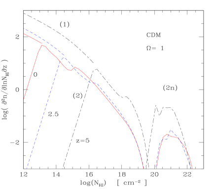
Figure 1: The contributions (1) corresponding to the Lyman-$\alpha$ forest (top left), (2) corresponding to the Lyman limit systems (central part) and $(2n)$ corresponding to the damped Lyman systems (bottom right), to the column density distribution, at $z=0$ (solid line), $z=2.5$ (dashed line) and $z=5$ (dot-dashed line).

Low column density lines ($N_{HI}<10^{15}$ cm^-2 at $z=2.5$ and $N_{HI}<10^{16}$ cm^-2 at $z=5$, on the left of the picture) correspond to low density areas and shallow potential wells (contribution (1)) with a roughly uniform density on scales smaller than the “damping” length $R_{d}$. The importance of this contribution decreases at small $z$ and shifts to low column densities because as time goes on most of the matter becomes embedded in deep potential wells, which are described by other regimes, while the average density of the universe declines. This translates into the redshift dependence of the upper column density $N_{HIupper}(z)$, see (17). These objects exist down to quite small column densities ($N_{HI}>10^{10}$ cm^-2 at $z=2.5$ and $N_{HI}>10^{12}$ cm^-2 at $z=5$), that is cloud dark matter masses as low as $10^{10}M_{\odot}$ at $z=0$ and $10^{6}M_{\odot}$ at $z=2.5$ and $z=5$. The associated absorption lines correspond to the Lyman$-{\alpha}$ forest.

Larger column densities, up to $N_{HIn}\sim 2\times 10^{19}$ cm^-2, are described by the regime (2). They are produced by virialized halos, which the line of sight intersects with an impact parameter much smaller than their radius but large enough so that the hydrogen is highly ionized. The low column density cutoff associated with this regime varies with redshift, as it corresponds to the upper limit of the regime (1) we described above, while the high column density cutoff is simply given by the ionization condition and is of the order of $N_{HIn}$, which is the column density at which the optical thickness is unity and whence is independent of $z$. Note that the regime (2$<$) corresponding to the rising part on the left of contribution (2), see eq.(27), plays no role since in this domain most observed lines are produced by forest clouds (regime (1)) described above. Indeed, the transition (2$>$) - (2$<$) coincides with the transition (1) - (2) as it should: we switch (almost) continuously from one class of objects to the other one. The absorption lines described by this regime (2) correspond to Lyman limit systems.

Finally, very high column densities (on the right of the figure), larger than $N_{HIn}$, correspond to lines of sight which intersect neutral cores. There is a gap in the distribution of column densities because the fraction of neutral hydrogen switches suddenly from $\sim 10^{-3}$ in ionized shells to $1$ in neutral cores (this is linked to the sharp change of the factor $\exp(-\tau)$ which behaves as an exponential of the column density). As we explained in Sect.3, we can see on the figure that the slope we obtain (for $N_{HI}\sim 10^{22}$ cm^-2) is steeper than the one we found for regime (2). These absorption lines correspond to damped Lyman systems.

Figure 2: The total column density distribution (summed over all contributions: Lyman-$\alpha$ forest, Lyman-limit and damped Lyman-$\alpha$ systems) at $z=3$. The data points are from Hu et al.(1995) (crosses) and from Petitjean et al.(1993) (rectangles).

We show in Fig.2 the total column density distribution at $z=3$ which results from the sum over all contributions. We can see that our model agrees reasonnably well with the observations, from $N_{HI}\sim 10^{13}$ cm^-2 up to $N_{HI}\sim 10^{22}$ cm^-2. In particular, we recover the under-abundance of lines at intermediate column densities $N_{HI}\sim 10^{15}-10^{16}$ cm^-2. This feature is also quite clear on Fig.1. It corresponds to the transition between populations (1) and (2). The gas embedded within galactic halos can cool and collapse (for deep potential wells $T>T_{0}$) which increases the column density along the line-of-sight (the neutral number density scales as the square of the baryonic density). As a consequence, clouds which would have produced column densities somewhat larger than $N_{HIupper}(z)$ actually lead to deeper absorption features. This produces an under-abundance of objects around $N_{HI}\sim 10^{15}$ cm^-2 at $z=2.5$.

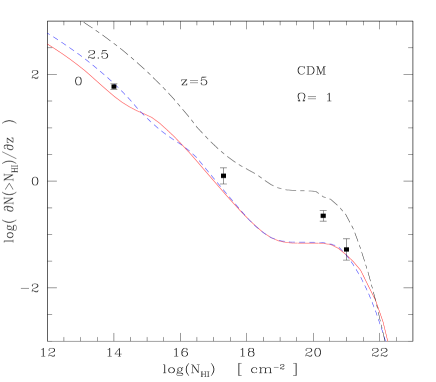
Figure 3: The total column density cumulative distribution at $z=0$ (solid line), $z=2.5$ (dotted line) and $z=5$ (dot-dashed line). The data are from Bechtold (1994) (Forest at $z=2.5$), Lanzetta et al.(1995) (Lyman limit systems at $z=2.6$) and Wolfe et al.(1995) (damped Lyman systems at $z=2.25$).

Fig.3 shows the total (summed over all contributions) column density cumulative distribution at $z=0,2.5$ and $5$. The flat part for $10^{19}<N_{HI}<10^{20}$ cm^-2 corresponds to the gap in Fig.1. This is also seen in numerical simulations (Katz et al.1996). We can see that the slope of the distribution function we obtain is again consistent with observations.

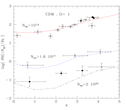
Figure 4: The evolution with redshift of the total column density cumulative distribution for $N_{HI}>10^{14}$ cm^-2 (upper curve), $N_{HI}>1.6\;10^{17}$ cm^-2 (intermediary curve) and $N_{HI}>2\;10^{20}$ cm^-2 (lower curve). The data points are from Bechtold (1994) (stars), Bahcall et al.(1996) (triangles), Giallongo et al.(1996) (filled squares), Kim et al.(1997) (open circles) and Lu et al.(1996) (filled circle) for $N_{HI}>10^{14}$ cm^-2; from Storrie-Lombardi et al.(1994) (crosses) for $N_{HI}>1.6\;10^{17}$ cm^-2; and from Wolfe et al.(1995) (filled squares) and Storrie-Lombardi et al.(1995) (cross) for $N_{HI}>2\;10^{20}$ cm^-2.

Table 1: Redshift evolution of the background UV flux $J_{21}(z)$ used in this article for both cosmologies (critical and open universe).

	$z=$0	1	2	3	4	5
$\Omega=$1	$J_{21}=$ 0.05	0.4	0.7	0.4	0.2	0.1
$\Omega_{0}=$0.3	0.05	0.5	0.8	0.4	0.2	0.1

The evolution with redshift of the total column density cumulative distribution is shown in Fig.4 for $N_{HI}>10^{14}$ cm^-2, $N_{HI}>1.6\;10^{17}$ cm^-2 and $N_{HI}>2\;10^{20}$ cm^-2. We can see in the figure that we can fit the data simultaneously for the 3 types of absorption lines which are representative of 3 different classes of objects: Lyman$-\alpha$ forest clouds, Lyman limit systems and damped Lyman systems, which are indeed described in our model by 3 different regimes. This builds our confidence in the validity of this model. Note that we could increase the number of damped systems by using a slightly larger $\sigma_{8}$ which does not significantly modify our results for limit and forest objects, as shown below in Sect.4.2. With $\Omega_{b}=0.04$, the values of the UV flux we use are shown in Tab.1. They are consistent with observations: Giallongo et al.(1996) find $J_{21}=0.5\pm 0.1$ for $1.7<z<4.1$, while Cooke et al.(1997) get $J_{21}=1^{+0.5}_{-0.3}$ for $2<z<4.5$, with no evidence for any redshift evolution within these intervals. At low redshifts $z\leq 1$ the UV flux shows a sharp drop (at $z=0$ Vogel et al.1995 find $J_{21}<0.07$ while Donahue et al.1995 get $J_{21}<0.033$). Moreover, the overall redshift dependance of $J_{21}(z)$ shown in Tab.1 is similar to the prediction of the usual models of galaxy formation from hierarchical scenarios where the radiation comes from stars and quasars (e.g. Haardt & Madau 1996). We can see in Fig.4 that we recover the observed break in the redshift evolution of the number density of lines at $z\sim 1.5$ (e.g. Jannuzi 1998). Indeed, at lower $z$ the number of lines with $N_{HI}>10^{14}$ cm^-2 remains constant while it slightly increases for Lyman-limit and damped systems. This break in the continuous decline with time of the number of forest lines due to structure formation which builds increasingly deep potential wells is produced by the sudden drop of the UV flux at low $z$. At low redshifts $z\sim 0$ we may overestimate the number of lines with $N_{HI}>1.6\;10^{17}$ cm^-2 and $N_{HI}>2\;10^{20}$ cm^-2 which come from galactic halos since we did not take into account star-formation which consumes (and may eject) some of the gas.

We can note that we manage to get a satisfactory agreement with observations for the column density distribution of Lyman-$\alpha$ clouds, while using $\Omega_{b}=0.04,\;H_{0}=$ 60 km/s, $\sigma_{8}=0.5$ and $J_{21}(z=2.5)=0.7$. On the other hand, numerical simulations need $\Omega_{b}>0.05$ for $J_{21}(z=2.5)>0.2$, $\sigma_{8}=0.79$, $\Omega=0.4$, $\lambda=0.6$, and $H_{0}=$ 65 km/s (Miralda-Escude et al.1996) or $\Omega_{b}>0.05$ for $J_{21}(z=2.5)>0.1$, $\sigma_{8}=0.7$, $\Omega=1$ and $H_{0}=$ 50 km/s (Katz et al.1996). These latter results would mean that it is difficult to satisfy the nucleosynthesis bounds with the observational estimates of $J_{21}$. The fact that we do not encounter such a serious problem here is rather encouraging and suggests, as we shall see below, that due to the very extended range of clouds (from weak potential wells to very deep halos) which contribute to a given $N_{HI}$ it is difficult to take into account properly all contributions (especially from the shallower clouds) in a simulation, which should thus usually underestimate the column density distribution function.

4.2 Influence of various parameters

As we explained in Sect.3, for all regimes the slope of the column density distribution only depends on the shape of the initial power-spectrum through $\omega$ and $\gamma$ (we take $\gamma=1.8$ but it could slightly depend on the slope $n$ of $P(k)$) as we can see in (13), (25) and (34). This constrains $n$ to be close to $-2$ hence both a CDM-like power-spectrum (since the local slope on the scales of interest is indeed close to $-2$) and a power-law power-spectrum with $n\simeq-2$ give satisfactory results. However, the normalization of the column density distribution depends on the UV flux $J_{21}$, as we noticed above, and on cosmological parameters. Indeed, we can see from Sect.3 that we have:

$$\left\{\begin{array}[]{l}{\displaystyle\left(\frac{\partial^{2}n}{\partial lnN_{HI}\partial z}\right)_{1}\propto\left(\frac{N_{HI}R_{d}}{n_{1}}\right)^{-(1-\omega)/2}\;[\overline{\xi}(R_{d})R_{d}]^{-\omega}h^{-1}}\\ \\ {\displaystyle\left(\frac{\partial^{2}n}{\partial lnN_{HI}\partial z}\right)_{2>}\propto\left(\frac{N_{HI}}{n_{1}}\right)^{-2/(2\gamma-1)}\;h^{-1}}\\ \\ {\displaystyle\left(\frac{\partial^{2}n}{\partial lnN_{HI}\partial z}\right)_{2n>}\propto\left(\frac{N_{HI}}{n_{2}}\right)^{-2/(\gamma-1)}\;h^{-1}}\end{array}\right.$$

with

$$n_{1}\propto\frac{T_{0}^{-0.75}(\Omega_{b}h^{2})^{2}}{J_{21}}\hskip 17.07182pt\mbox{and}\hskip 17.07182ptn_{2}\propto\Omega_{b}h^{2}$$ (38)

where we neglected the influence of the boundaries of the integrations over $x$. Fig.5 shows the influence of various parameters on the column density distribution. If we increase the normalization $\sigma_{8}$ of the power-spectrum hence $\overline{\xi}$ (dotted line in the figure), the number of Lyman-$\alpha$ forest lines decreases: clustering is more important (one is deeper into the non-linear regime) so that a larger fraction of the mass of the universe is within high density virialized halos which produce Lyman limit and damped systems. Simultaneously these two latter contributions increase, but this is not shown in (38) because we neglected the variation of the boundary in $x$. This increase is most important for highest column densities (massive damped systems) since these lines come from the rare high density halos which are in the exponential cutoff of the mass functions and whose abundance is very sensitive to the normalization of the power-spectrum (it enters as an exponential factor). On the other hand the number of Lyman-limit lines is nearly invariant because each of them is drawn from a large population of possible parent halos: increasing $\sigma_{8}$ means there are fewer low mass halos but more large mass halos and both effects nearly cancel each other. If the baryonic density parameter $\Omega_{b}$ gets higher (dot-dashed line) all contributions increase since there is more hydrogen available but the magnitude of this effect is not the same for all lines. Finally, if we increase $J_{21}$ the number of lines will decrease in all regimes since the neutral fraction of hydrogen is lower (dashed line). Once again, this is not seen in (38) for damped systems because it appears through the change of the boundaries over $x$: the deep cores of virialized halos are not influenced by a small increase of $J_{21}$, which only destroys the outer neutral shells. Indeed we can check in Fig.5 that the number of very large column density lines does not change. We note that a change of $\Omega_{b}$ or $J_{21}$ simply leads to a horizontal translation of the column density distribution for forest and Lyman limit absorbers. Indeed, the number and properties (for the dark matter) of these halos do not change, but a given region will produce a column density which evolves with the baryonic fraction ($\Omega_{b}$) and the neutral hydrogen fraction ($J_{21}$). This is no longer true for damped systems where a change of $\Omega_{b}$ or $J_{21}$ usually introduces new halos or removes the smallest ones. Moreover, we can see that the location of the gap between Lyman limit and damped systems is constant since it only depends on the photo-ionization cross-section, see (37).

Figure 5: The column density distribution as in Fig.1 at $z=2.5$ (solid line), with $J_{21}=3$ instead of 0.7 (dashed line), with $\Omega_{b}=0.1$ instead of $0.04$ (dot-dashed line), or with $\sigma_{8}=1.3$ instead of 0.5 (dotted line), at the same redshift.

Thus, we see that the normalization of the column density distribution does not depend only on the usual parameter $n_{1}$, and that a change of a given variable ($\Omega_{b},J_{21},T_{0}$ or $\sigma_{8}$) usually influences the three classes of objects described in Sect.3 in a different way. The dependence on $\sigma_{8}$ is very small for all values of interest except for the largest damped systems. This means that a power-spectrum normalized to the COBE data would also lead to a reasonable agreement with observations of Lyman-$\alpha$ clouds. The influence of $\Omega_{b}$ and $J_{21}$ is stronger, but it is degenerate for forest and Lyman limit lines through the combination $n_{1}$. Thus, for a given normalization of the power-spectrum, one could first derive $\Omega_{b}$ from observations of large damped systems, and then obtain $J_{21}$ from Lyman limit or forest absorbers, in order to match the data. However, we must emphasize that we have only one important “free” parameter in our model: $J_{21}$ (which must also be consistent with observations), since $P(k)$ and $\Omega_{b}$ are taken from consistent models of galaxies (VS II) and clusters which were already fully constrained by other sets of observations. This implies for instance that the abundance of the largest damped lines is given by these previous models. Indeed, as we explained above, these lines correspond simply to deep neutral shells of galactic halos, while the forest absorbers are new low-density objects (predicted by the same description of the non-linear density field, but in a different density regime)

4.3 Mass and circular velocity associated to different clouds

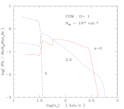
Figure 6: Evolution with redshift of the halo rotational velocity distribution function, for $N_{HI}=10^{17}$ cm^-2, at $z=0$ (solid line), $z=2.5$ (dashed line) and $z=5$ (dot-dashed line).

Our model yields the evolution with redshift of the halo rotational velocity (or mass, radius,..) distribution function, for a fixed column density. We define the halo circular velocity $v_{c}$ as:

$$v_{c}^{2}=\frac{{\cal G}M}{R}=\frac{4\pi}{3}{\cal G}\overline{\rho}(1+\Delta)R^{2}$$ (39)

and Fig.6 presents the case $N_{HI}=10^{17}$ cm^-2 at $z=0,2.5$ and $5$. The average halo rotational velocity (or mass) gets larger as time goes on, since gravitational clustering builds increasingly deep and massive potential wells. The sharp high velocity cutoff is not due to the multiplicity function of virialized halos but to the fact that very large and massive clouds cannot produce column densities as low as $N_{HI}=10^{17}$ cm^-2. In other words, looking at a specific $N_{HI}$ selects a finite range of parent halos (the contribution of larger clouds is not exactly zero because if the line of sight intersects such a halo very close to its external radius it can still produce a small column density, due to the small intersection length, but this occurs with a negligible probability as can be seen in the figure). The location of this cutoff does not evolve much from $z=0$ to $z=2.5$ because in this range clouds are defined by the cooling relation $R=R_{cool}$. Indeed, for a given halo the characteristic “minimum” column density on a line of sight is given by:

$$N_{HImin}\sim n_{1}(1+\Delta)^{2}R\sim\left(\frac{v_{c}}{R\sqrt{{\cal G}\overline{\rho}}}\right)^{4}n_{1}R$$ (40)

similarly to the calculation described previously for regime (1) clouds, see (10). Hence, a given column density selects a “maximum” rotational velocity:

$$v_{cmax}\sim R\sqrt{{\cal G}\overline{\rho}}\left(\frac{N_{HI}}{n_{1}R}\right)^{1/4}\propto\left(\frac{J_{21}(z)N_{HI}R_{cool}^{3}}{\Omega_{b}^{2}}\right)^{1/4}$$ (41)

which evolves slowly with $z$ through $J_{21}(z)^{1/4}$. In fact, at low $z$ this upper velocity cutoff increases with $z$ because of the sharp decline of $J_{21}(z)$ with time. Indeed, at $z\sim 2$ in order to observe a given column density (here $N_{HI}=10^{17}$ cm^-2) one must look through a deeper potential well (larger mass and density) defined by a higher $T$ and $v_{c}$ than at $z\sim 0$ because $J_{21}$ is much larger. On the other hand, at $z=5$ the clouds corresponding to $v_{cmax}$ for $N_{HI}=10^{17}$ cm^-2 are defined by the virialization condition $\Delta=\Delta_{c}$, so that we get:

$$v_{cmax}\propto\frac{J_{21}(z)}{\Omega_{b}^{2}}\frac{N_{HI}}{[(1+\Delta_{c})\overline{\rho}]^{3/2}}\propto J_{21}(z)(1+z)^{-9/2}$$ (42)

which decreases strongly at high redshift (note that we neglected the influence of the collapse factor $\lambda$). This behaviour can be understood very simply within the framework of the physical picture we developed in Sect.3 for Lyman-limit clouds, based on the association of these absorbers with galaxies. Indeed, at high redshift as time goes on the hierarchical clustering process builds increasingly deeper and more massive but lower density potential wells (the density of these halos scales as $(1+\Delta_{c})\overline{\rho}$), so that the rotational velocity attached to a given column density gets larger with time, as in (42). However, after some time (typically $z<1-2$) galaxies are no longer defined by the sole virialization constraint: massive galaxies are determined by a cooling constraint (VS II, Silk 1977, Rees & Ostriker 1977) which introduces a fixed length scale $R_{cool}$. As a consequence, the highest velocity associated with a given $N_{HI}$ does not evolve any more (except with the possible changes of the background UV flux $J_{21}$) which leads to the regime described by (41). In other words, at small redshift we identify Lyman-limit clouds with galaxies, and not with clusters of galaxies. This leads to a qualitative change in the behaviour of some physical properties. Thus, the “simple” hierarchical clustering scenario (coupled with a proper physical picture) can produce non-trivial histories, that is with qualitative discontinuities and amenable to observational checks. The lower cutoff is due to the fact that low velocity halos are described by regime (1): their density is roughly uniform over scales of the order of the “damping” length $R_{d}$ and they cannot produce large column density absorption lines. Thus, it corresponds to the virial temperature $T_{0}$ and shows (nearly) no evolution with redshift. The small discontinuity in the curve at $z=0$ around $v_{c}=60$ km/s corresponds to the transition from halos defined by $\Delta=\Delta_{c}$ (virialization constraint) to $R=R_{cool}$ (cooling constraint). The latter discontinuity thus has no physical meaning and is simply due to our interpolation procedure between these different regimes.

Figure 7: a) Evolution with redshift of the average rotational velocity of the halos associated to a given column density at $z=0$ (solid line), $z=2.5$ (dotted line) and $z=5$ (dot-dashed line). b) Evolution with redshift of the average mass of the halos associated to a given column density, for the same cases.

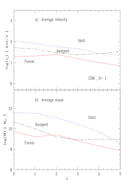
Figure 8: a) Evolution with redshift of the mean halo rotational velocity, for clouds defined by $N_{HI}=10^{14}$ cm^-2 (solid line), $N_{HI}=10^{17}$ cm^-2 (dashed line) and $N_{HI}=1.6\;10^{21}$ cm^-2 (dot-dashed line). b) Evolution with redshift of the mean halo mass, for the same cases.

We note in Fig.6 that the velocity distribution is quite extended, and that for $z\leq 2.5$ it is not far from uniform from 20 km/s up to 400 km/s. This is due to the fact that a given cloud may produce many different absorption features according to the value of the impact parameter $b$. Conversely, a given column density $N_{HI}$ may originate with a similar probability from many different clouds. Even at $z=0$, small velocity clouds ($v_{c}<100$ km/s) make up a sizeable fraction ($\sim 40\%$) of the total Lyman-$\alpha$ lines with $N_{HI}=10^{17}$ cm^-2. This could explain the fact that simulations with insufficient resolution produce fewer Lyman-limit systems than is required by the observations (Katz et al.1996) since it appears that one should resolve clouds down to $v_{c}\sim 20$ km/s.

Alternatively, we can consider the evolution with redshift of the mean halo rotational velocity or dark matter mass associated with a given column density. This is displayed in Fig.7 for $z=0,2.5$ and $5$. The feature at low velocity and mass corresponds to the transition between regimes (1) and (2), while the sudden change at $N_{HI}\sim 10^{20}$ cm^-2 is due to the transition from lines of sight intersecting ionized shells to those probing the neutral cores of deep halos. For any column density the average velocity and mass grow as time increases because the hierarchical clustering process builds deeper and more massive halos. At small $N_{HI}$ in regime (1), there is a unique correspondance between column density and velocity, or mass, see (10), which gives:

$$N_{HI}\propto(1+\Delta)^{2}\propto v_{c}^{2}\propto M^{2}$$ (43)

since the radius $R=R_{d}$ is constant. For larger $N_{HI}$ there is no longer such a unique relation, as different clouds can produce the same column density. The mean velocity or mass first increases with $N_{HI}$ and then reaches a plateau where it is nearly independent of $N_{HI}$. The rising part of the curve corresponds to the fact that larger column densities can be produced by deeper and more massive halos (as we described above for the high cutoff of the velocity distribution at fixed $N_{HI}$). Hence, as one looks for larger equivalent widths one adds to the population of parent halos new more massive and deeper clouds (while the minimum mass of the possible halos does not change since it is given by the fixed transition to the regime (1), one simply needs to draw lines of sight which pass closer to the center of this small potential well). As a consequence the average velocity (mass) increases with $N_{HI}$, until the high velocity (mass) cutoff gets larger than the typical velocity (mass) of objects which have collapsed at the considered redshift (this is where the cutoff of the mass functions comes in). Then, adding a new population of more massive halos when looking at a larger $N_{HI}$ only produces a negligible change in the mean velocity or mass because the number of these new clouds is very small.

Finally, there is a transition at $N_{HI}\sim 10^{20}$ cm^-2 where the average velocity and mass suddenly decrease to grow again later with $N_{HI}$. Indeed, for column densities slightly larger than $10^{20}$ cm^-2 we start to probe the neutral cores of virialized halos. The sharp change in the fraction of neutral hydrogen reflects that column densities $N_{HI}\sim 10^{20}-10^{21}$ cm^-2 can be produced by small clouds which were characteristic of the lowest Lyman-limit lines: the maximum velocity or mass allowed for a cloud to produce such a line decreases suddenly to the value corresponding to the transition between regimes (1) and (2), hence we recover the same mean velocity and mass, as can be seen in the figure. Then, exactly as occured for Lyman-limit systems, the average velocity (mass) first increases with $N_{HI}$ and finally reaches a plateau, due to the cutoff of the mass functions. This final velocity (mass) is larger than the one reached in the regime (2) for Lyman-limit lines, because the velocity (mass) distribution is more heavily weighted towards large velocity (mass). This is due to two factors. First, the neutral hydrogen density $n_{HI}$ is now proportional to the baryonic density and not to its square, see (20) and (31), which means that for a given cloud the change with the impact parameter $b$ of the column density is slower but also that for slightly larger clouds the impact parameter must increase faster in order to produce the same $N_{HI}$, which leads to a cross-section factor $b^{2}$ more heavily weighted towards large clouds. Second, the neutral radius $R_{n}$ grows faster than $R$, see (30), which again favors massive halos. Of course, this translates directly into the $R$ and $\Delta$ dependence of $\partial^{3}n/\partial lnN_{HI}\partial lnx\partial z$ in both regimes, see (24) and (33).

Fig.8 shows directly the redshift evolution of the average velocity or mass for 3 types of clouds, representative of the 3 classes of objects we described previously. The main feature is that for all clouds the mean velocity and mass decrease at higher redshift, since only weaker and smaller potential wells were formed at earlier times. This is not always true for the high column density $N_{HI}=1.6\;10^{21}$ cm^-2 because of the transition between ionized shells and neutral cores which introduces additional effects, as described above. This also explains why the average mass or velocity associated with this damped system is smaller at low $z$ than those characteristic of a lower column density Lyman-limit system.

4.4 Radius and impact parameter associated to various column densities

Figure 9: Evolution with redshift of the halo radius distribution function, for $N_{HI}=10^{17}$ cm^-2, at $z=0$ (solid line), $z=2.5$ (dotted line) and $z=5$ (long dashed line). The filled rectangle and the small ellipse represent the contribution of the clouds defined by the constraint $R=R_{cool}$ at $z=0$ and $z=2.5$, see text.

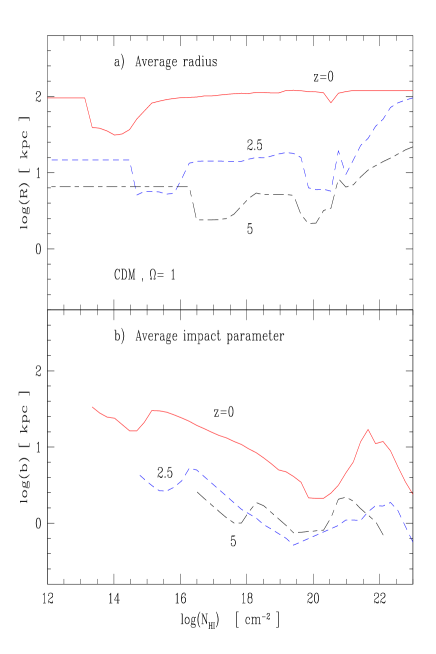
Figure 10: a) Evolution with redshift of the average radius and impact parameter of the halos associated to a given column density at $z=0$ (solid line), $z=2.5$ (dotted line) and $z=5$ (dot-dashed line). b) Evolution with redshift of the average neutral fraction of the halos associated to a given column density, for the same cases.

Figure 11: a) Evolution with redshift of the mean radius, for clouds defined by $N_{HI}=10^{14}$ cm^-2 (solid line), $N_{HI}=10^{17}$ cm^-2 (dashed line) and $N_{HI}=1.6\;10^{21}$ cm^-2 (long dashed line). b) Evolution with redshift of the mean impact parameter, for $N_{HI}=10^{17}$ cm^-2 (dashed line) and $N_{HI}=1.6\;10^{21}$ cm^-2 (dot-dashed line).

We present in Fig.9 the redshift evolution of the halo radius distribution function for a fixed column density $N_{HI}=10^{17}$ cm^-2 (here $R$ is the radius of the dark matter halo, i.e. without collapse). Note that massive halos are defined by a constant radius $R=R_{cool}$. In order to take into account this population in the picture, we also plotted in the figure the point $(R_{cool},\partial^{2}n/\partial lnN_{HI}\partial z)$ due to this contribution shown as a filled rectangle for $z=0$ and as a small ellipse for $z=2.5$. Thus, while the total contribution of halos defined by the virialization constraint $\Delta=\Delta_{c}$ is given by the integral over $lnN_{HI}$ of the curves shown in the figure, the total contribution of halos defined by the cooling constraint $R=R_{cool}$ is given by the ordinate of the point $(R_{cool},\partial^{2}n/\partial lnN_{HI}\partial z)$, multiplied by a Dirac $\delta(R-R_{cool})$ function, that in our more realistic model (VS II) is somewhat smeared out. The latter does not appear for $z=5$ because it is negligible. This allows us to get at once the proportion in number of both classes of objects. Thus, one can see that at $z=0$ the “$R_{cool}$ population” dominates so that most clouds associated with $N_{HI}=10^{17}$ cm^-2 have a dark-matter halo radius $R\sim R_{cool}=$ 120 kpc. At higher redshift the characteristic radius decreases but one can see that at $z=2.5$ the radius distribution is still quite extended, ranging from 4 kpc up to 120 kpc. The low radius cutoff corresponds to the transition with the regime (1) or to the influence of the cutoff radius $R_{cut}$ (indeed to observe a high column density through a small halo one should look close to the center where the gas density is high, however this is not always allowed since we remove lines of sight which would cross the galactic luminous core). It grows with time in parallel with the “damping” length $R_{d}$ and the lower cutoff $R_{c}$. Note that there is also in our present model an accumulation of clouds with radius $R_{d}$ (but various column densities) corresponding to population (1).

Fig.10 shows the average radius and impact parameter of the halos associated with a given column density at $z=0,2.5$ and $5$. The characteristic radius and impact parameter decrease at higher $z$ since virialized objects were smaller in the past. The panel a) shows the same features for the average radius of Lyman-limit and damped systems as those displayed in Fig.7 for the circular velocity or mass, that is at first increasing with $N_{HI}$ followed by a plateau, for the same reasons as those described previously. For Lyman forest clouds the radius $R=R_{d}$ is constant by definition. As shown in panel b), the impact parameter decreases for higher column densities, both for Lyman-limit and damped systems, since one has to probe deeper towards the center of the clouds to reach sufficiently high neutral hydrogen densities in order to obtain large $N_{HI}$ (the temporary increase within the range corresponding to Lyman-limit systems is due to the collapse of baryons which leads to larger $b$ for a given column density because the gas density is larger). The feature at $N_{HI}\sim 10^{20}-10^{21}$ cm^-2 is due to the transition between ionized shells and neutral cores, as usual. The impact parameter is not displayed for forest clouds (regime (1)) since it plays no role for this population and was not specifically defined (the radius is the sole relevant scale). We note that Bechtold et al.(1994) derive from observations at $z=1.8$ a radius $57<R<400$ kpc, with a median value of $R=130$ kpc, for clouds with $N_{HI}\sim 10^{14}$ cm^-2. Dinshaw et al.(1994) obtain similar values. The average radius we obtain in Fig.10 is smaller ($\sim 21$ kpc) but as shown in Fig.9 the radius distribution function is quite extended so that one indeed expects to observe clouds with a radius up to $\sim 100$ kpc. Moreover, as discussed in Appendix, our modelling is compatible with quite elongated filamentary clouds. The radius we refer to should be considered as the average intercept along the line-of-sight. However, if these very underdense clouds are filamentary, the distance at which two separate lines can hit the same cloud is much larger. So, we rather consider this offset as a possible manifestation of the non-sphericity of the absorption features.

Fig.11 shows the redshift evolution of the average radius and impact parameter for 3 column densities. One can see clearly the decrease at high $z$ of both length scales. The decline of $b$ is slower because at larger redshift the UV flux is lower while characteristic densities are higher, which tends to increase the impact parameter. We can also note that very different $N_{HI}$ have very close mean radii and impact parameters, while the radius and impact parameter distributions for a fixed column density are very extended, as was shown in Fig.9. Of course, this is due to the fact that a given $N_{HI}$ can be produced by a large range of clouds, so that very different column densities are in fact drawn from the same population of halos.

4.5 Metallicity

Figure 12: The average metallicity $Z_{h}$ of the halos associated to a given column density at $z=0$ (solid line), $z=2.5$ (dashed line) and $z=5$ (dot-dashed line).

Fig.12 shows the average metallicity (that is the abundance of oxygen or any other element mainly produced by SN II) of the halos associated with a given column density at $z=0,2.5$ and $5$. We obtain this metallicity from our model for the evolution of galaxies described in VS II. The latter is entirely consistent with the present study of Lyman$-\alpha$ absorption lines, as it uses the same description for the multiplicity functions of mass condensations. It also involves the same model of star-formation which enabled us (VS II) to get the luminosities of galaxies, as well as their metallicity, with no new parameter. In fact, within this framework we define three metallicities, corresponding to stars ($Z_{s}$), star-forming gas concentrated within the inner parts of galaxies ($Z_{c}$), and diffuse gas spread over the halo ($Z_{h}$) (corresponding to the two-component model of VS II). Lyman-limit lines, which arise when the line of sight intersects the outer ionized shells of a galactic halos, are characterized by $Z_{h}$, while for damped systems, corresponding to neutral cores, we should observe a metallicity in the range $Z_{h}$ to $Z_{c}$. We do not assign a metallicity to low column density forest lines, corresponding to regime (1), as they are associated with low density regions which may have not virialized yet. Observations by Lu et al.(1998) also find that there is a sharp drop in the metallicity of the gas (although for $C$) from $[C/H]\simeq-2.5$ for $N_{HI}>10^{14.5}$ cm^-2 downto $[C/H]<-3.5$ for $N_{HI}<10^{14}$ cm^-2, at redshifts $2.2<z<3.6$. Note that we predict a significant increase with $z$ of the column density corresponding with this transition. One may expect that diffusion processes (through winds or ejection of gas during violent mergers) would slightly lower the column density associated with this drop and would produce a non-zero metallicity for objects described by regime (1), which may also be enriched by a generation of population III stars. Naturally, the metallicity decreases at high redshift when star formation has not had enough time to synthesize many metals. At a given redshift, the metallicity increases with the column density, since high $N_{HI}$ implies deep and massive potential wells. In fact, it follows closely the behaviour of the rotational velocity as a function of the column density, see Fig.7, since the latter is related to the galaxy luminosity and metallicity as shown by observations (e.g. Zaritsky et al.1994). The sharp change for $N_{HI}\simeq 10^{20}$ cm^-2 corresponds again to the transition from ionized shells to neutral cores.

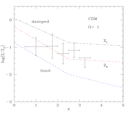
Figure 13: The redshift evolution of the average metallicity of the halos associated to $N_{HI}=10^{18}$ cm^-2 (dashed line) and $N_{HI}=10^{22}$ cm^-2 (dot-dashed lines). For damped systems two metallicities $Z_{c}$ and $Z_{h}$ are shown (see text). The data points are from Pettini et al.(1997) for the zinc metallicity of damped Lyman-$\alpha$ systems.

Fig.13 shows directly the redshift evolution of the metallicity associated with $N_{HI}=10^{18}$ cm^-2 (dashed line) and $N_{HI}=10^{22}$ cm^-2 (dot-dashed lines). For the latter case (damped systems) we display both metallicities $Z_{h}$ and $Z_{c}$, however the diffuse gas metallicity $Z_{h}$ should be the most relevant one. We can see that we obtain very good agreement with observations by Pettini et al.(1997). Moreover, we also obtain a large spread in metallicities (in the same way as the velocity distribution function was quite extended for a given column density, see Fig.6) which can be seen in Fig.12: although this picture only displays the average $Z_{h}$, the metallicity dispersion can be estimated from the sharp variation seen near $N_{HI}\sim 10^{21}$ cm^-2 where one probes different clouds. As was suggested by Pettini et al.(1997) in order to explain their observations, this is due to the fact that damped systems are drawn from a large population of parent galactic halos which have different star-formation histories and physical characteristics. This also provides a good check of the validity of our model.

4.6 Opacity

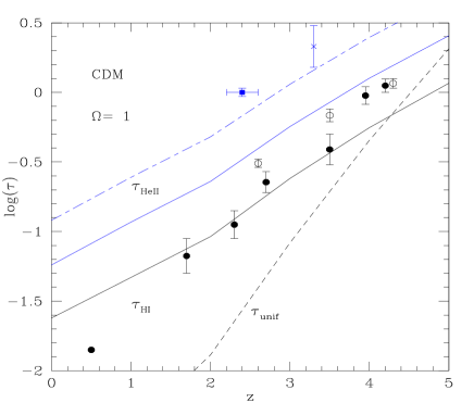
Figure 14: The evolution with redshift of the average hydrogen opacity $\tau_{HI}$ (lower solid line) and helium opacity $\tau_{HeII}$ (upper solid line and dot-dashed line, see text). The low dashed line shows the hydrogen opacity $\tau_{unif}$ which would be produced by a uniform IGM. The data points are from Press et al.(1993) (circles), Zuo & Lu (1993) (filled circles) for hydrogen, and from Davidsen et al.(1996) (filled rectangle) and Hogan et al.(1997) (cross) for helium.

Fig.14 displays the evolution with redshift of the average hydrogen opacity $\tau_{HI}(z)$. We can see that our result is roughly consistent with observations. In fact, this was already implied by Fig.2 and Fig.4 which showed that our model reproduces the evolution of the column density distribution. Indeed, the opacity is directly linked to the latter:

$$\tau_{HI}(z)=(1+z)\int\frac{\partial^{2}n}{\partial lnN_{HI}\partial z}\;\frac{W_{HI}}{\lambda_{\alpha}}\;dlnN_{HI}$$ (44)

where $W_{HI}$ is the equivalent width. As a comparison, the dashed line shows the opacity which would be produced by a uniform IGM:

$$\tau_{unif}(z)=\frac{\pi e^{2}f}{m_{e}\nu_{\alpha}}\;\frac{n_{1}(z)}{H(z)}$$ (45)

Thus, the clumpiness of the distribution of matter decreases the slope of the opacity as a function of redshift, as was already noticed by several authors (e.g. Bi & Davidsen 1997). Indeed, from (24) we expect for a constant UV background $J_{21}$ that

$$\tau_{HI}(z)\propto(1+z)\;\frac{dt}{dz}\;n_{0}(z)^{2/(2\gamma-1)}\;\left[\overline{\xi}^{-1}(\Delta_{c})\right]^{(3-2\gamma)/(2\gamma-1)}$$

If the clustering is stable, which is a good approximation for virialized halos, we obtain:

$$\tau_{HI}(z)\propto(1+z)^{3(6-\gamma)/(2\gamma)}=(1+z)^{3.5}\;\;\;\;\mbox{for}\;\;\;\;\gamma=1.8$$ (46)

which is already very close to observations: Dobrzycki & Bechtold (1996) find $\tau_{HI}=2.6\;10^{-3}(1+z)^{3.3}$, while $\tau_{unif}\propto(1+z)^{4.5}$. We can also obtain the helium II opacity provided we know the ratio $N_{HeII}/N_{HI}$. We used the curve $N_{HeII}/N_{HI}$ calculated by Haardt & Madau (1996) for $J_{21}=0.5$. In fact, as was already noticed by Miralda-Escude & Ostriker (1992) and Haardt & Madau (1996), and is easily checked numerically, most of the opacity comes from absorbers with $\tau\leq 1$ which are optically thin and verify $N_{HeII}/N_{HI}\simeq 1.8\;J_{912\AA}/J_{228\AA}$. Assuming that the radiation spectrum is a power-law with index $-2$, Haardt & Madau (1996) get $N_{HeII}/N_{HI}\sim 30$ for these clouds. We can see from Fig.14 that the helium opacity we obtain in this way (upper solid line) is smaller than the observations. This discrepancy may be due to a change in the slope of the ionizing radiation spectrum. In particular, the latter may show strong ionization edges at the HI, HeI and HeII ionization frequencies and display a step-like profile (see Gnedin & Ostriker 1997, Valageas & Silk 1998) which could significantly increase the ratio $N_{HeII}/N_{HI}$. Thus, we also show in Fig.14 the helium opacity we get with $N_{HeII}/N_{HI}=300$ (dot-dashed line). We note that, assuming that the $N_{HI}$ column density distribution follows a simple power-law in column density and redshift (chosen to be consistent with observations) and using $N_{HeII}/N_{HI}=100$, Zheng et al.(1998) find that at $z\sim 3$ half of the observed opacity is accounted for by clouds with $N_{HI}>10^{12}$ cm^-2. The helium opacity we obtain (dot-dashed line) is higher and consistent with the data because i) we use a larger ratio $N_{HeII}/N_{HI}$ and ii) the column density distribution we predict in our model extends down to small objects with $N_{HI}<10^{12}$ cm^-2, as shown by the lower cutoff $N_{HIlower}$ in (14) and (17). Thus, as noticed by Zheng et al.(1998) the large observed helium opacity strongly suggests that a significant part of the HeII absorption is produced by small density fluctuations which are below the observational limits for forest clouds detected through HI absorption. This population is also a natural prediction of our model.

4.7 Repartition of matter between different classes of objects

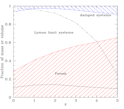
Figure 15: The evolution with redshift of the fraction of matter contained within Lyman-$\alpha$ clouds (for all column densities: whole lower dashed area, and for $N_{HI}<10^{11}$ cm^-2: dashed area under the lower solid line), Lyman limit systems (white area) and damped systems (upper dashed area). The area above the dot-dashed line which decreases sharply for $z>2.5$ is the volume fraction occupied by the Lyman-$\alpha$ forest clouds with $N_{HI}>10^{11}$ cm^-2 (Lyman limit and damped systems occupy a negligible volume fraction) while the area under this curve is the volume fraction occupied by the Lyman-$\alpha$ forest clouds with $N_{HI}<10^{11}$ cm^-2 and the very low-density regions (or voids) below the threshold $N_{HIlower}$, see (14), which do not produce sufficiently large absorption to be observed.

Finally, it is interesting to evaluate the fraction of the mass of the universe that is contained in the different populations of Lyman-$\alpha$ clouds (it is the same proportion for baryonic and non-baryonic matter in our model). This is displayed in Fig.15 as a function of redshift. We can see that the mass contained in Lyman limit and damped systems (associated with galaxies) increases as time goes on, together with structure formation via gravitational clustering. Moreover, the mass within damped systems is always very small, as it corresponds to the small deep cores of halos. It increases slightly with redshift because the density of all objects is larger at higher redshifts, which increases the relative masses of the neutral cores as compared to the halo masses. Simultaneously, the mass within the Lyman-$\alpha$ forest gets larger in the past when most of the matter present in the universe is contained in low density contrast areas which have not yet virialized (at the scale $R_{d}(z)$). We must note that even at $z=0$, these clouds form $\sim 30\%$ of the mass of the universe. Thus, at any redshift an important part of the mass of the universe is contained in small “low density” regions, which are not associated with galaxies or luminous matter. This matter can only be detected through absorption lines, as these small objects may not produce significant features in the velocity field. Note that a sizeable proportion of this mass is embedded within very low column density regions $N_{HI}<10^{11}$ cm^-2. Also, the detected -neutral- hydrogen is only a small (typically $10^{-5}$) fraction of the total baryon mass for Forest and Lyman-limit objects. Fig.15 shows the total baryon mass fraction, including thus the dominant, but unobserved, ionised fraction. Since we have assumed that the ratio of baryonic to total mass is constant, the mass fractions in Fig.15 also correspond to the total mass in the Lyman-$\alpha$ clouds. Note that the mass within damped Lyman systems is small: they nevertheless stick out prominently in the data because they correspond to totally neutral hydrogen, a given baryon mass fraction being thus ($\sim 10^{5}$ times) more efficient in producing the hydrogen absorption lines. The total mass fraction formed by these different populations is close to unity (the -negligible- mass fraction which we did not count corresponds to the luminous galactic cores behind which no quasar can possibly be seen). The volume fraction occupied by Lyman-$\alpha$ forest clouds with $N_{HI}>10^{11}$ cm^-2 is small for $z<2$ since in the highly non-linear universe most of the volume consists of very underdense regions. Lyman limit and damped systems occupy a negligible volume fraction.

4.8 Correlation function of various clouds

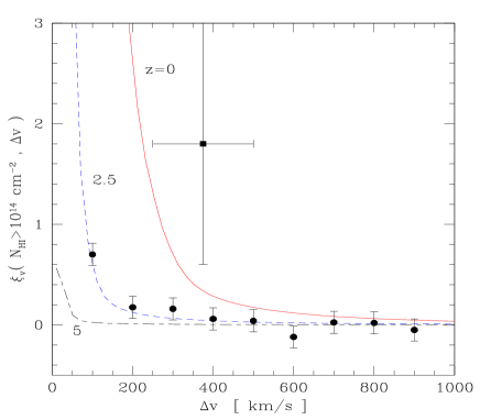
Figure 16: The two-point correlation function in velocity space for clouds with $N_{HI}\geq 10^{14}$ cm^-2, at the redshifts $z=0$ (solid line), $z=2.5$ (dashed line) and $z=5$ (dot-dashed line). The data points are from Cristiani et al.(1997) (dots) at $1.7<z<4$ and from Ulmer (1996) (rectangle) at $0<z<1.3$.

Finally, we show in Fig.16 and Fig.17 the redshift evolution of the two-point velocity correlation function $\xi_{v}$. In a fashion similar to Cristiani et al.(1997) we relate $\xi_{v}$ to the spatial correlation function $\xi_{\alpha}$ of Lyman-$\alpha$ clouds by:

$$\xi_{v}(v)=\int_{l_{min}}^{\infty}\xi_{\alpha}(r)P(v|r)dr$$ (47)

with $v>0$, $r>0$. The index $\alpha$ refers to the fact that $\xi_{\alpha}$ is linked to the matter correlation function $\xi$ through a bias factor $b^{2}$. We use for the conditional probability $P(v|r)$ a gaussian of width $\sigma_{v}$ centered on $Hr=v$, where $H(z)$ is the Hubble constant and $\sigma_{v}$ a characteristic velocity dispersion of the considered pair of clouds. The low cutoff $l_{min}$ is simply the sum of both cloud radii $l_{min}=R_{1}+R_{2}$. For small clouds $\sigma_{v}\ll v$ so that $P(v|r)$ is narrowly peaked at $r=v/H$, while for large clouds $\sigma_{v}\geq v$ so that the integral is dominated by its lower cutoff, due to the divergence at small $r$ of $\overline{\xi}(r)$. Thus, we write:

$$\xi_{v}(N_{HI1},N_{HI2},v)\sim\xi_{\alpha}(N_{HI1},N_{HI2},r)$$ (48)

with

$$r=\mbox{Max}\left(R_{1}+R_{2},\frac{v-\sigma_{v}}{H(z)}\right)$$ (49)

for the velocity correlation function of two lines of column densities $N_{HI1}$ and $N_{HI2}$. We estimate the pair velocity dispersion as $\sigma_{v}=(v_{c1}+v_{c2})/2$, where $v_{ci}$ is the mean circular velocity associated with a given $N_{HIi}$, which was described previously in Fig.7 and Fig.8. Next, we need to obtain the bias parameter $b^{2}(N_{HI1},N_{HI2})$. Within the framework of the scale-invariance of the many-body matter correlation functions $\xi_{p}({\bf r}_{1},...,{\bf r}_{p})$ which led to the mass function (4) one can show that at large distances $r\gg R_{1},R_{2}$, in the highly non-linear regime, the bias characteristic of two objects factorizes and is a function of the sole parameter $x$ introduced in Sect.2, see Bernardeau & Schaeffer (1992). Thus we write:

$$\xi_{\alpha}(N_{HI1},N_{HI2},r)=b(x_{1})b(x_{2})\overline{\xi}(r)$$ (50)

with

$$x\ll 1:\;b(x)\propto x^{(1-\omega)/2}\hskip 14.22636pt\mbox{and}\hskip 14.22636ptx\gg 1:\;b(x)\propto x$$ (51)

In our case, a fixed column density $N_{HI}$ may arise from many different clouds, so as for the velocity dispersion we shall simply use a mean $x_{i}$ for each $N_{HIi}$. Note that the previous relation (50) breaks down for $r\sim(R_{1}+R_{2})$, but in view of the approximations involved (through the use of various averages) we shall use it down to $r=(R_{1}+R_{2})$ where it should still provide a reasonable estimate. Finally, since observations usually refer to the mean velocity correlation function above a given threshold in column density, we are led to define:

$$\begin{array}[]{l}{\displaystyle\xi_{v}(>N_{HI},v)=\left(\int_{N_{HI}}^{\infty}\frac{dN}{N}\eta(N)\right)^{-2}}\\ \\ {\displaystyle\hskip 28.45274pt\times\int_{N_{HI}}^{\infty}\frac{dN_{1}}{N_{1}}\frac{dN_{2}}{N_{2}}\eta(N_{1})\eta(N_{2})\xi_{v}(N_{1},N_{2},v)}\end{array}$$ (52)

where $\eta(N_{HI})=\partial^{2}n/\partial lnN_{HI}\partial z$.

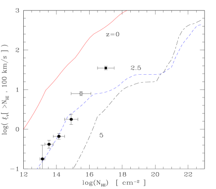
Figure 17: The dependence on the column density threshold of the two-point correlation function $\xi_{v}(>N_{HI},100$ km/s) for the redshifts $z=0$ (solid line), $z=2.5$ (dashed line) and $z=5$ (dot-dashed line). The data points are from Cristiani et al.(1997) (disks) for $1.7<z<4$, Songaila & Cowie (1996) (circle) at $2.66<z<3.62$ and Petitjean & Bergeron (1994) (rectangle) at $z\sim 2.5$. These two latter points are derived from CIV metal systems.

We compare in Fig.16 the correlation function $\xi_{v}(>N_{HI},v)$ we obtain in this way to observations, for a column density threshold $N_{HI}>10^{14}$ cm^-2 as a function of velocity. We can see that our predictions agree reasonably well with observations, both at low redshift (data from Ulmer 1996) and at high redshift (data from Cristiani et al.1997). Fig.17 shows the dependence on the column density threshold $N_{HI}$ of the correlation function $\xi_{v}(>N_{HI},v)$ for the redshifts $z=0,2.5$ and 5. We reproduce the observed increase with $N_{HI}$ of $\xi_{v}(>N_{HI},v)$ over the range spanned by the data. For small column densities, Lyman forest clouds described by the regime (1), the correlation function measured for a fixed velocity separation increases with $N_{HI}$ because a higher column density corresponds to a deeper potential well, that is a higher parameter $x$, hence a larger bias $b(N_{HI})$. Since for these low-density clouds the circular velocity is small, as seen in Fig.7 and Fig.8 (because their virial temperature $T$ is lower than $T_{0}$ by definition) the spatial separation is simply constant: $r=v/H(z)$. Larger column densities (Lyman-limit systems) come from deeper potential wells with a higher circular velocity so that the bias parameter keeps increasing while the separation $r$ becomes influenced by the velocity factor $\sigma_{v}$, hence decreases slowly down to $R_{1}+R_{2}$. Thus the correlation function grows with $N_{HI}$. As was the case for the mean radius, mass or velocity associated to a given column density, $\xi_{v}(>N_{HI},v)$ reaches a flat plateau for sufficiently large Lyman-limit systems, when different $N_{HI}$ are drawn from the same population of parent halos. Finally, there is also a rising part and a higher plateau for damped systems, as in the previous studies for the velocity or mass. We can notice that there is not a deep gap around $N_{HI}\sim 10^{20}$ cm^-2, contrary to these former cases, because the correlation function $\xi_{v}(>N_{HI},v)$ involves an integral over column densities above a given threshold, see (52), which smooths the curves. In fact, as can be inferred from Fig.2 for instance, the correlation function for lines above $10^{19}$ cm^-2 is dominated by the contribution of column densities around $N_{HI}\sim 10^{21}$ cm^-2.

5 Open universe: $\Omega_{0}=0.3\;,\;\Lambda=0$

5.1 Column density distribution

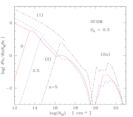
Figure 18: The contributions (1) corresponding to the Lyman-$\alpha$ forest (top left), (2) corresponding to the Lyman limit systems (central part) and $(2n)$ corresponding to the damped Lyman systems (bottom right), to the column density distribution, at $z=0$ (solid line), $z=2.5$ (dashed line) and $z=5$ (dot-dashed line) from bottom to top.

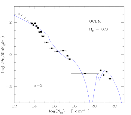
Figure 19: The total column density distribution (summed over all contributions) at $z=3$. The data points are from Hu et al.(1995) (points) and from Petitjean et al.(1993) (circles).

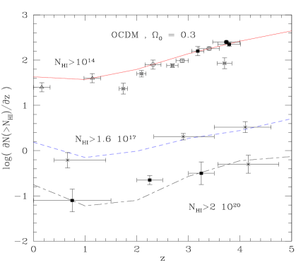
Figure 20: The evolution with redshift of the total column density cumulative distribution for $N_{HI}>10^{14}$ cm^-2 (upper curve), $N_{HI}>1.6\;10^{17}$ cm^-2 (intermediary curve) and $N_{HI}>2\;10^{20}$ cm^-2 (lower curve). The data points are from Bechtold (1994) (crosses), Bahcall et al.(1996) (circles), Giallongo et al.(1996) (filled circles), Kim et al.(1997) (rectangles) and Lu et al.(1996) (triangle)for $N_{HI}>10^{14}$ cm^-2; from Storrie-Lombardi et al.(1994) (dashed crosses) for $N_{HI}>1.6\;10^{17}$ cm^-2; and from Wolfe et al.(1995) (filled circles) and Storrie-Lombardi et al.(1995) (dashed crosses) for $N_{HI}>2\;10^{20}$ cm^-2.

For a low-density universe, $\Omega_{0}=0.3,\;\Lambda=0$, we can perform the same analysis. Thus, Fig.18 shows the column density distribution at $z=0,2.5$ and $5$, while Fig.19 compares our predictions with observations at $z=3$. Fig.20 presents the evolution with redshift of the total column density cumulative distribution for $N_{HI}=10^{14}$ cm^-2, $N_{HI}=1.6\;10^{17}$ cm^-2 and $N_{HI}=2\;10^{20}$ cm^-2. We can see that we obtain good agreement with the data, similarly to the previous case of a critical universe. This is not really surprising, since as we noticed earlier, provided the model-independent properties of the multiplicity function discussed in Sect.2 are satisfied, the main features of the column density distribution we get, and the corresponding properties of the Lyman-$\alpha$ clouds, come from the basic characteristics of the physical model we built to define and recognize these absorbers. Of course, the normalization of the power-spectrum plays some role, see Fig.5 for instance, especially for damped systems, but it is not the dominant factor for other column densities. Thus, the values of $J_{21}(z)$ we use (see Tab.1) are similar in both cases and consistent with observational estimates.

5.2 Opacity

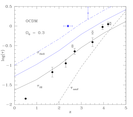
Figure 21: The evolution with redshift of the average hydrogen opacity $\tau_{HI}$ (lower solid line) and helium opacity $\tau_{HeII}$ (upper solid line and dot-dashed line). The low dashed line shows the hydrogen opacity $\tau_{unif}$ which would be produced by a uniform IGM. The data points are from Press et al.(1993) (circles), Zuo & Lu (1993) (filled circles) for hydrogen, and from Davidsen et al.(1996) (filled rectangle) and Hogan et al.(1997) (cross) for helium.

Finally, Fig.21 presents the redshift evolution of the helium and hydrogen opacities. Of course we obtain results very close to the case of a critical universe since the column density distributions were already similar.

6 Conclusion

In this article we have developed an analytical model for the redshift evolution of Lyman-$\alpha$ absorbers. It is based on a description of gravitational structures which can handle objects defined by various density contrast thresholds, both negative and positive, assuming that the many-body correlation functions are scale-invariant. This allows us to go beyond the usual Press-Schechter approach, which is in principle restricted to just-virialized halos. This is a key ingredient for modeling Lyman-$\alpha$ absorption lines since they arise from a wide variety of objects: from underdense clouds to the high-density neutral cores of deep potential wells. Once such a tool to count gravitational dark matter structures is properly devised, in a consistent way so as to keep track of all the mass in the universe while avoiding double-counting, one still needs to specify a physical model in order to associate with each neutral hydrogen column density observed on a line of sight the possible objects responsible for this feature.

Similarly to Rees (1986) we consider that large $N_{HI}$ lines come from virialized clouds which we associate with galactic halos. The external shells ionized by the background UV flux lead to Lyman limit lines, while the neutral cores (protected from this UV flux by self-shielding) correspond with damped Lyman systems. A single cloud produces a very extended range of possible column densities, as a function of the impact parameter of the line of sight, due to its steep density profile ($\rho\propto r^{-\gamma}$ for our model of spherical clouds). This has important consequences since it implies that very different $N_{HI}$ are drawn from almost the same population of parent halos. Thus, it leads to characteristic features (plateaus and correspondence between various regimes) in curves such as the mean halo rotational velocity or mass as a function of the column density. Note that these objects are not defined, as is often done, by the sole constant density threshold $\Delta_{c}\sim 177$ as we also take into account a cooling constraint, together with the common virialization criterium.

Moreover, in addition to this population of clouds identified with galactic halos, we include a second class of lower density objects. These correspond to weak potential wells where baryonic density fluctuations are erased over scales of the order of the “damping” length $R_{d}$. Thus, contrary to the former class of clouds, the impact parameter plays no significant role and a given object will produce a specific column density. These halos, defined by the length scale $R_{d}$, cover a large range of densities, from very underdense regions to density contrasts $\Delta\sim 40$, and correspond to the Lyman forest lines. As discussed in Appendix, the features giving rise to these Lyman forest lines need not be real spherical objects and can be treated simply as absorbing features along the line-of-sight within our framework. Thus, although the mean intersecting length $R_{//}$ of these regions with a given line-of-sight is of order $R_{d}$ (which is why we also call $R_{d}$ the radius of these “objects”), the actual extension of such a filament can be much larger. As a consequence, the distance at which two separate lines of sight can hit the same cloud can be much larger than $R_{d}$. This explains why the “radius” $R_{d}$ we obtain is much smaller than some lengths obtained from observations of close quasar pairs.

As we noticed above, this wide variety of physical objects makes it indeed necessary to use a description of gravitational structures which allows one to consider in a unified manner a large range of density contrasts and scales. For instance, one cannot study Lyman forest clouds, nor high column densities at low $z$, by looking only at just-virialized objects, while smoothing the density field over the Jeans length prevents one from modelling Lyman-limit and damped systems which correspond to very high density contrasts at similar scales.

We also have compared the redshift evolution of the column density distribution and the hydrogen and helium opacities predicted by our model to observations, for a critical CDM universe as well as for an open universe $\Omega_{0}=0.3$. In both cases we get a good agreement with the data, while the main new parameter is the UV flux $J_{21}$. Indeed, the slope of the column density distribution and the relative characteristics associated to various $N_{HI}$ are mainly given by the physical model itself we built to identify Lyman-$\alpha$ clouds. We can also note that the amplitude of the UV flux we need is consistent with observations and usual models of structure formation.

Next, we used the power given by such an analytical approach to study the influence of various parameters like the normalization of the power-spectrum $\sigma_{8}$, the baryonic density parameter $\Omega_{b}$ and the amplitude of the UV flux. Thus, we showed how their influence varies according to the considered regime (forest, Lyman limit or damped systems) which in principle allows one to remove for instance the degeneracy associated with $\Omega_{b}^{2}/J_{21}$ when one is restricted to the forest and Lyman limit contributions. Note however that $\Omega_{b}$ and $\sigma_{8}$ are not really free parameters, since they are chosen so as to be consistent with an earlier model of galaxy formation. Then, we looked at detailed predictions of our model such as the mean halo mass or radius associated with a given hydrogen column density, as well as the velocity or radius distribution themselves for fixed $N_{HI}$. This shows that, due to the role of the impact parameter, such distributions are very extended so that even at $z=2.5$, the characteristic halo rotational velocities associated for instance with $N_{HI}=10^{17}$ cm^-2 cover a large range from $\sim$ 10 km/s up to 500 km/s. This also means that one would need very high-resolution numerical simulations to take into account the contributions produced by all these clouds. Moreover, we showed that even within the framework of the “simple” hierarchical structure formation scenario the redshift evolution of quantities like the maximum halo rotational velocity assigned to a given $N_{HI}$ displays a qualitatively non-uniform behaviour, due to the role of non-gravitational processes which introduce additional length or temperature scales. Taking advantage of the fact that our model for Lyman-$\alpha$ absorbers is part of a broader unified description of the structures formed in the universe, including galaxies, we used the model of galaxy formation and evolution developed earlier (VS II) to obtain the characteristic metallicities of Lyman-limit and damped systems. We again obtain a good agreement with observations, which confirms the validity of our approach (both for galaxies and Lyman-$\alpha$ clouds !).

Finally, we considered the redshift evolution of the mass and volume fractions formed by the various populations of clouds. We note that, contrary to some numerical studies, we managed to obtain reasonable agreement with the observational column density distribution function together with a UV flux $J_{21}=0.7$ at $z=2.5$ consistent with observations using a baryonic density parameter $\Omega_{b}=0.04$ that is close to nucleosynthesis bounds. As we noticed previously this could be explained by the very wide range of parent clouds which contribute to a given $N_{HI}$, so that it is difficult for simulations to keep track of all objects (particularly weak potential wells) and not to underestimate the column density distribution function. Our formalism is also very convenient for studying the correlation function of Lyman-$\alpha$ clouds. We again obtain results in good agreement with observations, both for the redshift evolution and for the dependence on column density of the amplitude of the correlation function.

Thus, we conclude that the physical picture on which our model is based should provide a good description of the processes at work in the real universe, since its predictions agree with observations for many different quantities. Moreover, it allows one to get very detailed results and keep track of the influence of various processes, while building a unified consistent picture of the universe. Of course, in order to obtain a simple analytical model we had to make some approximations: for instance we consider spherical clouds (although we tried to correct this in a crude way in the regime where it may make a difference: at the transition between ionized shells and neutral cores) and we did not include the effects of star formation, that is likely to be at the origin of the UV flux. Since the latter is a key ingredient at all redshifts, it would be interesting to see whether our model of galaxy formation can produce the UV flux needed to match the observational constraints on Lyman-$\alpha$ clouds, this will be the subject of a forthcoming article (Valageas & Silk 1998). However, the amplitude $J_{21}$ we used is always consistent with observational estimates, so that the results obtained in this article are quite robust in this respect. Eventually, the detailed predictions of our model will have to be checked against more precise future data, in order to narrow the range of possible physical and cosmological parameters.

APPENDIX

Appendix A Objects versus density fluctuations

In Sect.3.1 we have calculated the number of Lyman$-\alpha$ forest absorbers along the line-of-sight as if the latter were actual distinct objects of size $R_{d}$. We show here that there is a very simple condition for such a calculation to be equivalent to the more direct statistics of the density fluctuations along the line-of-sight. Indeed, both approaches are intimately related and there is a single condition for the latter to reduce to the former one. This also shows that we take into account all the matter along each line-of-sight (we do not restrict ourselves to the highest density peaks neglecting low density regions).

The estimate (2) of the number of objects of size $R$ and mass $M$ is based on the statistics of the counts in cells of size $R$. If the fluctuating density field corresponds to a density $\rho(r)$, that is to a deviation $\delta(r)=\frac{\rho(r)-\overline{\rho}}{\overline{\rho}}$, the statistics of the counts-in-cells is nothing but the statistics of $\int\delta(r)d^{3}r$ within the cell. On the other hand, the statistics of the density field along the line-of-sight, that we are interested in here, is the statistics of the smoothed density field over the scale $R_{d}$, that is the statistics of the average $\delta_{d}=\int\delta(r)d^{3}r/V_{d}$ where $V_{d}$ is the volume over which we average. The probability for the random variable $\delta_{d}$ to take a given value $\delta$ at a point $r$ along the line-of sight thus has the same expression as the probability to find the overdensity $\delta$ within a cell of size $R_{d}$, the latter being given by the statistics of the counts-in-cells (Balian & Schaeffer 1989). It can be written:

$$p(\delta)d\delta=\frac{1}{\overline{\xi}(R_{d})}xh(x)\frac{dx}{x}$$ (53)

where $x=\frac{1+\delta}{\overline{\xi}(R_{d})}$. The associated column density is

$$N_{HI}=2\;n_{HI}\;R_{//}=2\;n_{1}\;x^{2}\;\overline{\xi}(R_{d})^{2}\;R_{//}$$ (54)

where $R_{//}$ is the length along the line-of-sight over which the contrast $\delta$ is maintained before the density drops to a negligible value. We must recall here that at the small scales we consider here, all the matter is within very dense spots of negligible volume surrounded by a nearly empty space. This is discussed in great detail by Balian & Schaeffer (1989) and more recently, in connection with the present work, by Valageas & Schaeffer (1997). This equation can be usefully compared to (10). Also, the number of occurences per redshift interval $dz$ is:

$$dn=c\frac{dt}{dz}\frac{dz}{R_{//}}p(\delta)d\delta=c\frac{dt}{dz}\frac{dz}{R_{//}}\frac{1}{\overline{\xi}(R_{d})}xh(x)\frac{dx}{x}$$ (55)

The column density distribution then reads

$$\left(\frac{\partial^{2}n}{\partial lnN_{HI}\partial z}\right)_{1}=\frac{1}{2}\frac{1}{R_{//}}c\frac{dt}{dz}\frac{1}{\overline{\xi}(R_{d})}xh(x)$$ (56)

an expression that is written for a fixed value of $N_{HI}$ and in which $x$ thus depends on $R_{//}$ through (54). This equation again can be usefully compared to (12). In the power-law regime $h(x)\propto x^{\omega-2}$ which is relevant here, it differs from the latter by a factor

$$\frac{4}{3}\frac{R_{d}}{R_{//}}\left(\frac{2}{3}\frac{R_{d}}{R_{//}}\right)^{\frac{\omega-1}{2}}$$ (57)

Provided $R_{//}$ is governed by the scale $R_{d}$, this factor is of order unity and our previous estimate in Sect.3.1 leads to the same results as in the present case.

Next, we can argue that $R_{//}$ actually is of order $R_{d}$. Indeed, since density fluctuations (and the density of typical matter condensations) increase at smaller scales (following the increase of the two-point correlation function $\overline{\xi}(R)$) one expect the smallest scale at which fluctuations exist (which we called $R_{d}$) to dominate. This can also be seen from a simple model where we assume overdensities to be in the form of long straight cylinders of radius $R_{d}$ and length $L$ with $L\gg R_{d}$. Then, a given filament can produce different column densities as the angle $\theta$ between its main axis and the line-of-sight varies (along with the length $R_{//}\sim R_{d}/\sin\theta$). Indeed, a straightforward calculation along the lines of Sect.3 gives:

$$\begin{array}[]{l}{\displaystyle\left(\frac{\partial^{3}n}{\partial lnN_{HI}\partial lnR_{//}\partial z}\right)\sim\frac{1}{L}c\frac{dt}{dz}\;\overline{\xi}^{\;-\omega}\left(\frac{N_{HI}}{2n_{1}R_{//}}\right)^{(\omega-1)/2}}\\ \\ {\displaystyle\hskip 56.9055pt\times\;\left(1+\frac{L}{R_{//}}\right)\frac{R_{d}}{R_{//}}\left[1-\left(\frac{R_{d}}{R_{//}}\right)^{2}\right]^{-1/2}}\end{array}$$ (58)

This shows that the number of lines, for a fixed column density $N_{HI}$, is dominated by the small values of $R_{//}$: the value of the integral of (58) over $R_{//}$ to get $\partial^{2}n/\partial lnN_{HI}\partial z$ is determined by the lower cutoff $R_{d}$. In other words, in order to achieve a given $N_{HI}$ it is more likely to look through a higher density region of size $R_{d}$ than to look through a lower density filament almost exactly along its main axis. This justifies our calculation and the equivalence of (56) with (12). On the other hand, we note that the mean intersecting length $R_{//}$ obtained from (58), that is assuming a straight cylinder, is of order $L$ (the integral now diverges at large scales). However, although long overdense filaments are quite likely to be present, a description in terms of a Rayleigh-Levy random walk (with direction jumps over distances of order $R_{d}$) rather than a long straight cylinder is certainly more accurate. In this case, the average intercept is barely twice the thickness $R_{d}$ and all the moments are finite, of order $R_{d}$. In simple words, even if the distribution of low density contrasts is filamentary, it is sufficiently irregular, with direction jumps over distances $R_{d}$, made of $N$ blobs of size $R_{d}$, but coherent over a distance $L\sim N^{1/2}R_{d}\gg R_{d}$, so as to allow us to describe the distribution of intercepts along the line-of-sight as if these features were distinct objects. Thus, the description of the number of Lyman forest lines in terms of the fluctuating density field and our description in terms of “objects” of size $R_{d}$ are equivalent.

The main difference of such a description in terms of filamentary clouds rather than spherical objects is the distance at which two different lines-of-sight can cross the same cloud. Indeed, whereas the intercept $R_{//}$ is of order $R_{d}$, the coherence of the absorption features for two neighbouring lines-of-sight will be of order $L\gg R_{d}$.