The time averaged TeV energy spectrum of Mkn 501 of the extraordinary 1997 outburst as measured with the stereoscopic Cherenkov telescope system of HEGRA

Abstract

During the several months of the outburst of Mkn 501 in 1997 the source has been monitored in TeV $\gamma$-rays  with the HEGRA stereoscopic system of imaging atmospheric Cherenkov telescopes. Quite remarkably it turned out that the shapes of the daily $\gamma$-ray  energy spectra remained essentially stable throughout the entire state of high activity despite dramatic flux variations during this period. The derivation of a long term time-averaged energy spectrum, based on more than 38,000 detected TeV photons, is therefore physically meaningful. The unprecedented $\gamma$-ray  statistics combined with the 20% energy resolution of the instrument resulted in the first detection of $\gamma$-rays from an extragalactic source well beyond 10 TeV, and the first high accuracy measurement of an exponential cutoff in the energy region above 5 TeV deeply into the exponential regime. From 500 GeV to 24 TeV the differential photon spectrum is well approximated by a power-law with an exponential cutoff: ${\rm d}N/{\rm d}E=N_{0}\,(E/1\,{\rm TeV})^{-\alpha}\,\exp{(-E/E_{0})}$, with $N_{0}=(10.8\leavevmode\nobreak\ \pm 0.2_{\rm stat}\leavevmode\nobreak\ \pm 2.1_{\rm sys})\cdot 10^{-11}\,\rm cm^{-2}s^{-1}TeV^{-1}$, $\alpha=1.92\leavevmode\nobreak\ \pm 0.03_{\rm stat}\leavevmode\nobreak\ \pm 0.20_{\rm sys}$, and $E_{0}=(6.2\leavevmode\nobreak\ \pm 0.4_{\rm stat}\leavevmode\nobreak\ (-1.5\leavevmode\nobreak\ +2.9)_{\rm sys})\,\rm TeV$. We summarize the methods for the evaluation of the energy spectrum in a broad dynamical range which covers almost two energy decades, and study in detail the principal sources of systematic errors. We also discuss several important astrophysical implications of the observed result concerning the production and absorption mechanisms of $\gamma$-rays  in the emitting jet and the modifications of the initial spectrum of TeV radiation due to its interaction with the diffuse extragalactic background radiation.

1 Introduction

Mkn 501, an active galactic nucleus (AGN) at a redshift $z=0.034$, was discovered several years ago as a faint source of TeV $\gamma$-radiation (Quinn et al. quin:96 (1996) ; Bradbury et al. brad:97 (1997)). In 1997 it turned into a state of high activity, unique in both its strength and duration. The TeV emission of the source from March to September 1997 was characterized by a strongly variable flux. It was on average more than three times larger than the flux of the Crab Nebula, the strongest known persistent TeV source in the sky. Fortunately, the time period of the outburst coincided with the source visibility windows of several ground-based imaging atmospheric Cherenkov telescopes (IACTs) designed for the detection of very high energy (VHE) cosmic $\gamma$-rays. Thus almost continuous monitoring of Mkn 501 in TeV $\gamma$-rays  with several IACTs (CAT, HEGRA, TACTIC, Telescope Array, Whipple) located in the Northern Hemisphere was possible (e.g. Protheroe et al. prot:98 (1997)).

The observations of Mkn 501 by the HEGRA stereoscopic IACT system during this long outburst made a detailed study of the temporal and spectral characteristics of the source possible, based on an unprecedented statistics of more than 38,000 TeV photons (Aharonian et al. 1999a ; hereafter Paper 1). The “background-free” detection of $\gamma$-rays  , with an average rate of several hundred $\gamma$-rays  per hour (against $\approx 20$ background events caused by charged cosmic rays), allowed us to determine statistically significant signals for $\leq 5$ minute intervals during much of the 110 h observation time, spread over 6 months. Moreover, it was possible to monitor the energy spectrum of the source on a daily basis. Within the errors the energy spectrum maintained a constant form over the range from 1 TeV to 10 TeV. This was the case even though the flux varied strongly on time scales $\leq 1$ day. We believe that this is an important result, and it was to some extent unexpected.

The diurnal spectra exhibit a power-law shape at low energies (between 1 TeV and several TeV), with a gradual steepening towards higher energies (Paper 1). Such a spectral form could not be unequivocally ensured in the first analysis which was performed during the period of activity of the source, since the systematic errors of the recently commissioned stereoscopic system of HEGRA were not well studied at this time. As a consequence, the energy spectrum could not be determined more precisely than implied by a power law fit (Aharonian et al. 1997a ), even though the tendency for a gradual steepening of the observed spectra was noticed (Aharonian et al. 1997b ). The results of Paper 1 and the new results in a broader energy interval presented below are based on detailed systematic studies (see Paper 1 and Konopelko et al. kon:99 (1999)), and extend and supersede these previous results. This allowed us to come to the definite conclusion that the spectrum determined in the energy region from 1 to 10 TeV steepens significantly (Paper 1). A similar tendency has been found also by the Whipple (Samuelson et al. samuel:98 (1998)), Telescope Array (Kajino et al. 1999, private communication), and CAT (Djannati-Atai et al. CATcorrelation (1999)) groups. Independent spectral measurements by the HEGRA telescopes CT1 and CT2 will be published elsewhere.

Apart from its astrophysical significance, the constancy of the spectral shape has the important practical consequence that it allows to measure the spectrum with small statistical errors also in the energy regions below 1 TeV and above 10 TeV. Indeed, the low photon statistics of the detector in both ”extreme” energy bands (towards low energies basically due to the decrease of the detector’s collection area; towards high energies due to the steep photon spectrum) can be drastically increased by using the data accumulated over the whole period of observations.

In Sect. 2 we describe the HEGRA stereoscopic system and the specific form of the data analysis, based on Monte Carlo simulations of both, the air showers and the detection system. The data sample is the same as in Paper 1 and is described in Sect. 3. A detailed study of the systematic errors in the spectrum derivation is contained in Sect. 4; most of this methodology was actually developed in the context of the Mkn 501 data analysis. We believe that this is the first study of this kind. The experimental results are then presented in Sect. 5, whereas Sect. 6 attempts a first discussion. This discussion concentrates on the $\gamma$-ray results of Sect. 5 and what one can learn from them alone. A multiwavelength analysis is clearly outside the scope of this paper. Our conclusions are contained in Sect. 7.

Readers only interested in the astrophysical results, should skip Sect. 2-4 and proceed to Sect. 5.

2 The HEGRA system of imaging atmospheric Cherenkov telescopes

2.1 The HEGRA Cherenkov telescope system

The VHE $\gamma$-ray observatory of the HEGRA collaboration consists of six imaging atmospheric Cherenkov telescopes (IACTs) located on the Roque de los Muchachos on the Canary island of La Palma, at 2200 m above sea level. A prototype telescope (CT1) started operation in 1992 and has undergone significant hardware upgrades since then. This telescope continues to operate as an independent instrument. The stereoscopic system of Cherenkov telescopes consists of five telescopes (CT2 - CT6), and has been taking data since 1996, initially with three and four telescopes, and since 1998 as a complete five-telescope system. Four of the telescopes (CT2, CT4, CT5, CT6) are arranged in the corners of a square with roughly 100 m side length, and one telescope (CT3) is located in the center of the square. During 1997, when the data discussed in this paper were taken, CT2 was still used as stand alone detector.

The telescopes have an 8.5 m² tessellated reflector, focusing the Cherenkov light onto a camera with 271 photomultipliers (PMTs), covering a field of view of $4.3^{\circ}$ in diameter. A telescope is triggered when the signal in at least two adjacent PMTs exceeds an amplitude of 10 (before June 1997) or 8 (after June 1997) photoelectrons; in order to trigger the CT system and to initiate the readout of data, at least two telescopes have to trigger simultaneously. Typical trigger rates are in the 10-16 Hz range. The PMT signals are digitized and recorded by 120 MHz Flash-ADCs. The telescope hardware is described by Hermann (her:95 (1995)); the trigger system and its performance are reviewed by Bulian et al. (bul:98 (1998)).

2.2 Reconstruction of air showers with the HEGRA IACT system

The routine data analysis (see Paper 1 for details) includes a screening of data to exclude data sets taken at poor weather conditions or with hardware problems. In particular, the mean system trigger rate proved to be a sensitive diagnostic tool. Reconstruction of data involves the deconvolution of Flash-ADC data (Hess et al. hess:98 (1998)), the calibration and flat-fielding of the cameras, the determination of Hillas image parameters, and the reconstruction of geometrical shower parameters based on the stereoscopic views of the air shower obtained with the different telescopes (Daum et al. daum:97 (1997), Aharonian et al. 1997a ). The characteristic angular resolution for individual $\gamma$-rays is $0.1^{\circ}$; by sophisticated procedures $\gamma$-ray sources can be located with sub-arcminute precision (Pühlhofer et al. pul:97 (1997)).

The separation of hadronic and electromagnetic showers is based on the shape of the Cherenkov images, in particular using the width parameter. The width of each image is normalized to the average width of a $\gamma$-ray image for a given impact parameter of the shower relative to the telescope, and a given image intensity. Here, impact distances are obtained from the stereoscopic reconstruction of the shower geometry. Cuts are then applied to the mean scaled width obtained by averaging the scaled width values over telescopes. For a point source both the pointing information and the image shape information are used. Each of them provides a cosmic-ray background rejection of up to 100.

The reconstruction of the energy of air showers is based on the relation between the shower energy and the image intensity (size) at a given distance from the shower axis (Aharonian et al. 1997c ). This relation is tabulated based on Monte Carlo simulations, with the zenith angle of the shower as an additional parameter. The distance between a given telescope and the shower core is known from the stereoscopic reconstruction of the shower, with a typical precision of 10 m or less, for not too distant showers. The energy estimates from the different telescopes are then averaged, taking into account the slightly different sensitivities of the telescopes. These sensitivities are calibrated to 1% by comparing the light yield in two telescopes for events with cores halfway between the two telescopes (Hofmann hof:97 (1997)). According to Monte Carlo simulations, this energy reconstruction provides an energy resolution of 15% to 20%, depending on the selection of the event sample.

2.3 Monte Carlo simulations of air showers and of the telescope response

Any quantitative analysis of IACT data has to rely on detailed Monte Carlo simulations to evaluate the detection characteristics of the instrument.

The simulation of air showers and of Cherenkov light emission (Konopelko et al. kon:99 (1999)) includes all relevant elementary processes. On their trajectory to the detector, photons may be lost by ozone absorption, Mie scattering, and Rayleigh scattering. Atmospheric density profiles, ozone profiles and aerosol densities have been checked against local experimental data where available (e.g. Hemberger mark:98 (1998)).

On the detector side, the simulations include the wavelength dependence of the mirror reflectivity, of the light collection system, and of the PMT quantum efficiency. The point spread function of the mirror system is modeled after measurements of images of bright stars. The readout electronics is simulated in significant detail. PMT output waveforms are modeled by superimposing the response to single photoelectrons, with their relative timing and amplitude smearing. These signals are then sampled, quantitized, and fed into the same analysis path as regular Flash-ADC data. The simulation includes the measured saturation effects both in the PMT/preamplifier and in the Flash-ADC. Details concerning the Monte Carlo simulation used here, the performance of the system, and the comparison with experimental data are described by Konopelko et al. (kon:99 (1999)).

3 The Mrk 501 data sample

The analysis is based on the same data sample as used in Paper 1, corresponding to a total exposure time of 110 h, between March and October of 1997. Mrk 501 was observed in the so-called wobble mode, with the source positioned $\pm 0.5^{\circ}$ in declination away from the optical axis of the telescopes, alternating every 20 min. For background subtraction, an equivalent region displaced by the same amount in the opposite direction is used. The separation of $1^{\circ}$ of these on-source and off-source regions is large compared to the angular resolution of the telescope system. In total, the sample comprises about 38,000 $\gamma$-ray events.

To select $\gamma$-ray candidates, the same loose cuts were applied as in Paper 1. In particular, the reconstructed shower direction had to be within $0.22^{\circ}$ from the source, and the mean scaled width parameter had to be less than 1.2. Events were accepted up to a maximum impact parameter of 200 m from the central telescope CT3. Events with larger impact parameters frequently suffer from truncated images in the cameras and, due to small angles between the stereo views, have larger uncertainties on the shower parameters. Since the analysis presented in the following emphasizes the control of systematic errors, it was felt that in this case the advantage of having clean events and a well-defined effective area at large energies – basically all events within the 200 m radius trigger above a few TeV – outweighs the gain in statistics which could have been achieved by accepting all events . For the following analysis a software threshold of two or more triggered telescopes, each with at least 40 recorded photoelectrons was used.

Properties of this Mrk 501 data sample were examined in detail in Paper 1.

4 Determination of energy spectra and sources of systematic errors

Compared to single IACTs, stereoscopic IACT systems permit drastic reduction of systematic errors, in particular for tasks like the precision determination of energy spectra. Using the redundant information provided by the multiple views, essentially all relevant characteristics, such as the radial distribution of Cherenkov light or the trigger probabilities of the telescopes can be verified experimentally (see also Hofmann hof:97 (1997)). Simultaneous sampling of the intensity of the Cherenkov light front in different locations emphasizes the calorimetric nature of the energy determination, and reduces the effect of local fluctuations. Finally, given the unambiguous reconstruction of the shower geometry and the fact that at energies of one TeV virtually all events within 100 m from the central telescope trigger the system, and that above a few TeV almost all events within 200 m trigger, the effective detection area above 1 TeV can be basically defined by pure geometry, without relying on simulations. Only the threshold region requires a critical consideration.

Under ideal conditions, the differential energy spectrum of the incident radiation is determined as

$$\phi(E)={r(E)\over\eta(E)A(E)}\,,$$ (1)

where $r(E)$ is the measured rate of $\gamma$-rays of energy $E$ after background subtraction, $A(E)$ is the effective detection area and $\eta(E)$ is the efficiency of the cuts applied to isolate the signal and to suppress the background. The effective area and the cut efficiencies are usually derived from Monte Carlo simulations.

A complication arises from the finite energy resolution, described by the response function ${\cal R}(E^{\prime},E)$, the probability that a $\gamma$-ray of energy $E$ is reconstructed at an energy $E^{\prime}$. The measured rate is hence given by the convolution

$$r(E^{\prime})=\int dE\leavevmode\nobreak\ {\cal R}(E^{\prime},E)\leavevmode\nobreak\ \eta(E)A(E)\phi(E)\,.$$ (2)

Eq. 2 can no longer be trivially inverted to yield $\phi(E)$. Options to find $\phi(E)$ include the explicit deconvolution using a suitable algorithm, which will usually make some assumption concerning the smoothness of the spectrum. Another approach is to assume a certain functional form for the shape of the spectrum, and to determine free parameters such as the flux and the spectral index from a fit of Eq. 2 to the data. Finally, one can absorb the effect of the energy smearing into a modified effective area $A$, defined such that Eq. 1 holds. The latter approach is the simplest, but has the disadvantage that now $A$ depends on the assumed shape of the spectrum. However, with the $<20\%$ energy resolution provided by the HEGRA CT system, shape-dependent corrections are negligible for most practical purposes, and results are stable after one iteration. Therefore, while both other techniques were pursued, the final results are based on this third method.

The typical energy dependence of the effective area is shown in Fig. 1. Below 1 TeV, the effective detection area rises steeply with energy, and then saturates at around $10^{5}$ m². The saturation reflects the cut on a maximum distance from the central telescope of 200 m.

Figure 1: Effective area of the HEGRA IACT system as a function of energy, for vertical $\gamma$-rays. The saturation at $10^{5}$ m² at high energies reflects the cut in impact distance at 200 m relative to the central telescope. The uncertainty of the effective area in the threshold region caused by a 5% variation of the detection threshold and by the interpolation in zenith angles is shown by the hatched area. The corresponding systematic error on the effective area is $\sim 50$% at 500 GeV and $\sim 10$% at 1 TeV.

The technical implementation of the energy reconstruction and flux determination is described in detail in Paper 1. Compared to the brief discussion given above, a main complication for real data arises from the dependence of $A$ on the zenith angle $\theta$, which varies during runs and from run to run. In order to be able to interpolate between Monte Carlo-generated effective areas at certain discrete zenith angles, a semi-empirical scaling law is exploited, which relates the effective areas at different zenith angles. The variation of zenith angles with time is accounted for through replacing Eq. 1 by the sum over all events recorded within the observation time $T$

$$\phi(E)={1\over T}\sum_{events}{1\over\eta(E,\theta)A(E,\theta)}$$ (3)

where each event is weighted with the appropriate effective area, given its energy and zenith angle. Note that for each period of a certain hardware configuration a set of effective areas is used which has been determined from the Monte Carlo simulations which model in detail the specific hardware performance, i.e. which take into account the trigger configuration and the mirror point spread function (see Paper 1).

The key aspect in a precise and reliable determination of $\gamma$-ray spectra is the control of systematic errors. Sources of systematic errors include, e.g.,

• Systematic errors in the determination of the absolute energy scale.

• Deviations from the linearity of the energy reconstruction, caused e.g. by threshold effects at very low energies, and possible saturation effects in the PMTs or the electronics at very high energies.

• Systematic errors in the determination of the effective area $A$; particularly critical is the threshold region, where $A$ is a very steep function of $E$.

• Systematic errors in the determination of the (energy-dependent) efficiency of the angular and image shape cuts.

As discussed in detail in Appendix A, a non-accurate modeling of the detector response or the atmospheric transmission possibly results in 1) a shift in the energy scale of the reconstructed $\gamma$-ray spectrum, and 2) a distortion of the shape of the spectrum. Most systematic uncertainties, e.g. mirror reflectivities and PMT quantum efficiencies, exclusively contribute to an error of the energy scale. The calculations in Appendix A show that the curvature of the spectrum is reconstructed correctly provided that the Monte Carlo simulations accurately model the correlation between the detector threshold and the reconstructed energies including the fluctuations involved. If the Monte Carlo description of this correlation is incorrect, the energies reconstructed in data and the effective areas computed from Monte Carlo simulations do not match. A shift of the reconstructed energies by a factor $(1+\epsilon)$ relative to the effective area $A$ used for the evaluation of the spectrum results in a flux error of

$${\Delta\phi\over\phi}\approx{\Delta A(E)\over A(E)}\approx\epsilon\leavevmode\nobreak\ {\mbox{d}\ln{A(E)}\over\mbox{d}\ln{E}}\leavevmode\nobreak\ \leavevmode\nobreak\ \leavevmode\nobreak\ .$$ (4)

The flux error is potentially large in the threshold region, where $A$ varies quickly with $E$, $A\propto E^{\beta}$ with $\beta\simeq 6$ and $\Delta\phi/\phi\approx 6\epsilon$, but is negligible at high energies, where $A$ is constant, and is simply governed by the geometrical cuts (see Fig. 1).

The remainder of this section is dedicated to a discussion of the various sources of systematic errors.

4.1 Reliability of the determination of the shower energy

A crucial input for the determination of shower energies is of course the expected light yield as a function of core distance. Since the average core distance varies significantly with energy, inadequacies in the assumed relation will not only worsen the energy resolution, but will systematically distort the spectrum. With the redundant information provided by a system of Cherenkov telescopes, it is possible to actually measure the light yield as a function of the distance from the shower core and to verify the simulations (Aharonian et al. ahar:98b (1998)). Briefly, the idea is to select showers with a fixed impact parameter relative to a telescope A, and with a fixed light yield in this telescope. This provides a sample of showers of constant energy, and now the light yield in other telescopes can be measured as a function of core distance. Fig. 2 shows the characteristic shape of the light pool for $\gamma$-ray showers, which is well reproduced by the simulation; this holds also for the variation of the shape with shower energy and zenith angle (Aharonian et al. ahar:98b (1998)).

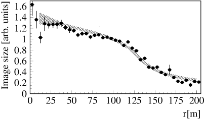
Figure 2: Measured light yield as a function of distance to the shower core for $\gamma$-ray showers in the energy range of about 0.9 to 1.8 TeV compared with Monte Carlo simulations (hatched band). Note that the light yield assigned to images depends on the field of view of the camera, and on the definition of “image” pixels; the data should not be compared to “raw” simulations not including such effects.

A second key ingredient in the energy determination is the reconstruction of the core location. Unlike in the case of the angular resolution, where it is easy to show that the simulation reproduces the data by comparing the distribution of shower directions relative to the source with the simulations, a direct check of the precision of the core reconstruction is not possible. However, noting that two telescopes suffice for a stereoscopic reconstruction, one can split up the four-telescope system into two systems of two telescopes and compare the results (Hofmann hof:97 (1997)). Figure  3a illustrates the difference in core coordinates between the two subsystems for data and for the Monte Carlo simulations. As can be recognized the Monte Carlo simulations accurately predict the distribution of the distances between the two cores. Under the assumption that the two measurements are uncorrelated and that the reconstruction accuracy achieved with two telescopes is the same for two telescope and four telescope events the width of the difference distribution should be $\sqrt{2}$ times the resolution of a two-telescope system. By this means, the 2 telescope resolution is determined to be $14\leavevmode\nobreak\ {\rm m}\leavevmode\nobreak\ /\leavevmode\nobreak\ \sqrt{2}\leavevmode\nobreak\ \approx\leavevmode\nobreak\ 10$ m. The Monte Carlo simulations show, that this reconstruction accuracy does indeed agree nicely with the true reconstruction accuracy for 2 telescope events.

Figure 3: (a) Difference in the $x$ coordinate of the shower core as measured by independent subsystems of two telescopes for events where all four telescope triggered. Showers are selected to provide a minimum stereo angle of $20^{\circ}$ in each subsystem, and a maximum core distance of 200 m from the central telescope. Points show the data, the dashed line the simulation, and the full line a Gaussian fit to the data with a width of 14 m. (b) Comparison of the energies measured by the two subsystems. The width of the Gaussian fit is 25%. Same cuts as in (a).

The same technique can be used to study the energy resolution (Fig. 3b; see also Hofmann hof:97 (1997)). Also here the data is in excellent agreement with the simulations. In this case, the Monte Carlo studies predict, that the energies measured with the two subsystems are considerably correlated: assuming uncorrelated estimates, an energy resolution of $25\%\leavevmode\nobreak\ /\leavevmode\nobreak\ \sqrt{2}\leavevmode\nobreak\ =\leavevmode\nobreak\ 18\%$ is inferred; the Monte Carlo simulations predict a true energy resolution for two telescope events of 23%. On the basis of simulations, fluctuations in the shower height can be identified as the origin of this correlation. Work is ongoing to use the stereoscopic determination of the shower height to improve the energy resolution. The excellent agreement between data and Monte Carlo simulations confirms that the experimental effects entering the energy determination are well under control, and that consequently the estimate of the energy resolution based on the simulations is reliable.

4.2 The absolute energy scale

The absolute energy calibration of IACTs is a significant challenge, lacking a suitable monoenergetic test beam. Factors entering the absolute energy calibration are the production of Cherenkov light in the shower, the properties and the transparency of the atmosphere, and the response of the detection system involving mirror reflectivities, PMT quantum efficiencies, electronics calibration factors etc. So far, mainly three techniques were used to calibrate the HEGRA telescopes:

• The comparison between predicted and measured cosmic-ray detection rates. Given the integral spectral index of 1.7 for cosmic rays, an error $\epsilon$ in the energy scale results in an error of $1.7\epsilon$ in the rate above a given threshold. Apart from the slightly different longitudinal evolution of hadronic and of $\gamma$-ray induced showers, this test checks all factors entering the calibration. The Monte Carlo simulations reproduce the measured cosmic-ray trigger rates within 10% (Konopelko et al. kon:99 (1999)). The IACT system was furthermore used to determine the flux of cosmic-ray protons in the 1.3 to 10 TeV energy range (Aharonian et al. 1999b ). The measured flux of protons

  $${\rm d}N_{\rm p}/{\rm d}E=(0.11\pm 0.02_{\rm stat}\pm 0.05_{\rm sys})\times$$ (5)

  $$\hskip 14.22636ptE^{-2.72\pm 0.02_{\rm stat}\pm 0.15_{\rm sys}}\leavevmode\nobreak\ \leavevmode\nobreak\ \leavevmode\nobreak\ \rm s^{-1}sr^{-1}m^{-2}TeV^{-1}$$

  excellently agrees with a fit to the combined data of all other experiments, indicating that systematics are well under control and that the assigned systematic errors – partially related to the energy scale – are rather conservative.

• Given the measured characteristics of the telescope components such as mirrors or PMTs, the sensitivity of the telescopes can be determined with an overall error of 22%.

• Using a distant, calibrated, pulsed light source, an overall calibration of the response of the telescope and its readout electronics could be achieved, with a precision of 10% (Fraß et al. frass:97 (1997)).

The last three techniques have to rely on the Monte Carlo simulations of the shower and of the atmospheric transparency. While Monte Carlo simulations have converged and different codes produce consistent results, details of the atmospheric model and assumptions concerning aerosol densities can change the Cherenkov light yield on the ground by about 8% (Hemberger 1998).

Within their errors, all calibration techniques are consistent. Overall, we believe that a 15% systematic error on the energy scale is conservative, given the state of simulations and understanding of the instrument. Based on the comparison with cosmic-ray rates, one would conclude that the actual calibration uncertainty is below 10%.

4.3 The threshold region and associated uncertainties

As discussed earlier in detail, the threshold region is very susceptible to systematic errors. In the sub-threshold regime events trigger only because of upward fluctuations in the light yield, and energy estimates tend to be biased towards larger values. Fig. 4 shows the mean reconstructed energy as a function of the true energy for a sample of simulated events at typical zenith angles. Note that for the 1997 data set we have a noticeable number of detected $\gamma$-rays events below 500 GeV. However in this energy region the bias is so strong that a reliable correction is no longer possible. Therefore spectra will only be quoted above this energy.

Figure 4: Mean reconstructed shower energy as a function of the true energy for showers incident under 20^∘ zenith angle, also showing the rms errors of the energy reconstruction.

Figure 5: Size-distributions of $\gamma$-ray induced air showers for data and simulations for two of the four telescopes. The data is from a period of a certain trigger configuration, namely “Data-period I” of Paper 1, and the Monte Carlo simulations used the telescope specific single pixel trigger probability as function of signal amplitude derived from this data (Mkn 501 data, background subtracted, Monte Carlo weighted according to the results in Sect. 5).

The first major source of systematic errors at low energies is the detailed modeling of the triggering process. In the simulation great emphasis was placed on the correct description of the pixel trigger probabilities as a function of signal amplitude. For each trigger configuration and for each telescope this dependence has been derived from air shower data using the recorded information about which pixels of a triggered telescope surpassed the discriminator threshold and which pixels did not. As discussed above and in Appendix A, the onset of the size-distribution provides a sensitive test of the quality of the simulation. Fig. 5 shows the measured and simulated size-distribution for two telescopes for a certain trigger configuration (“Data-period I” of Paper 1). For our current best simulations, fits to the rising edges of the size-distributions indicate for the individual telescopes and the different trigger configurations deviations of the size scale between data and Monte Carlo on the 5% level. For conservatively estimating the systematic error on the shape of the Mkn 501 spectrum, we allow for a $\pm$5% correlated shift of the thresholds of all four telescopes. The resulting uncertainties in the effective detection area $A$ are indicated in Fig. 1; as expected, $A$ significantly changes in the threshold regime, but remains constant well above threshold.

Random threshold variations (Gaussian-distributed with a width of 15%) between individual pixels were found to be of relatively small influence compared to the systematic threshold shifts.

As another source of systematic errors of special importance in the threshold region, the accuracy of the energy reconstruction for zenith angles between the discrete simulated zenith angles ($\theta=0^{\circ}$, $20^{\circ}$, $30^{\circ}$, $45^{\circ}$) has been considered. Imperfections in the scaling law used to relate the Cherenkov light yield at different zenith angles $\theta$ could result in a systematic shift of the reconstructed energy at intermediate values of $\theta$. To test the description, the energy of the Monte Carlo showers with $\theta=30^{\circ}$ was determined with the light yield tables of the $0^{\circ}$- and $45^{\circ}$-showers and the result was compared to the result based on using the $30^{\circ}$ light yield table. The systematic shift of the reconstructed energies was about 5% below 1 TeV and 2% above 1 TeV; based on this and other studies we believe that using the full set of simulations, systematic shifts in the reconstructed energy are below 5% and 2%, below and above 1 TeV respectively.

The modified effective area used for the determination of the spectrum slightly depends on the assumed source spectrum. At the lowest and at the highest energies the source spectrum can not be determined with high statistical accuracy. For energies below 1 TeV we conservatively estimate the corresponding uncertainty in the modified effective area, by varying the spectral index of an assumed source spectrum dN/dE$\propto$E^-α from $\alpha=1.5$ to $\alpha=3$. At the highest energies above 15 TeV we vary the assumed source spectrum from a broken power law to a power law with an exponential cutoff, both specified by fits to the data. In addition we explore the statistical significance of the $\gamma$-ray excess at the highest energies by a dedicated $\chi^{2}$-analysis (see Sect. 5).

In the threshold region of the detector the total systematic error is dominated by the systematic shift of the telescope thresholds and by the possible systematic shift in the reconstructed energy due to the zenith angle interpolation. The total systematic error is computed by summing up the individual relative contributions in quadrature.

4.4 Saturation effects at high energies

Figure 6: The mean signal in the peak pixel, hot₁, as a function of the image size, for data (full points) and simulations (open points).

The PMTs and readout chains of the HEGRA system telescopes provide a linear response up to amplitudes of about 200 photoelectrons. At higher intensities, nonlinearities of the PMT become noticeable, and also the 8-bit Flash-ADC saturates. With typical signals in the highest pixels of 25 photoelectrons per TeV $\gamma$-ray energy, the effects become important for energies around 10 TeV and above.

Saturation of the Flash-ADC can be partly recovered by using the recorded length of the pulse to estimate its amplitude, effectively providing a logarithmic characteristic (Hess et al. hess:98 (1998)). The saturation characteristics of the PMT/preamplifier assembly have been measured, and a correction is applied. These nonlinearities and the Flash-ADC saturation are included in the simulations. As a very sensitive quantity to test the handling of saturation characteristics, the dependence of the pulse height in the peak pixel on the image size emerged (Fig. 6). Data and simulations are in very good agreement up to pixel amplitudes exceeding 10³ photoelectrons, equivalent to $>$50 TeV $\gamma$-ray showers. Older versions of the simulations, which did not properly account for PMT/preamp nonlinearities, showed marked deviations for size-values above 10³.

Independent tests of saturation and saturation corrections were provided by omitting, both in the data and in the simulation, the highest pixels in the image, and by comparing event samples in different ranges of core distance and zenith angle. The saturation effect is non-negligible only at very high energies, namely $E\geq 15\,\rm TeV$. However, all tests show that given the quality of our current simulations, systematic errors induced by saturation effects even in this energy region are yet small compared to the statistical errors.

4.5 Efficiency of cuts

Among the sources of systematic errors, the influence of cuts

Figure 7: Efficiency of the cut on the shower direction relative to the Mrk 501 location after the software threshold of at least 40 photoelectrons in two or more telescopes (a), and of the shape cuts used to enhance $\gamma$-rays (b), as a function of energy. Full points show the measured efficiencies, open points the results of the Monte Carlo simulations. Efficiencies determined from data can be larger than one due to background fluctuations.

is less critical. The large flux of $\gamma$-rays from Mrk 501 combined with the excellent background rejection of the IACT system allows to detect the signal essentially without cuts. In the analysis, one can afford to apply only rather loose cuts, which keep over $80\%$ of all $\gamma$-rays; only at the lowest energies, a slightly larger fraction of events is rejected. Since only a small fraction of the signal is cut, the uncertainty in the cut efficiency is a priori small; in addition, the efficiency can be verified experimentally by comparing with the signal before cuts, see, e.g., Fig. 7. The cut efficiencies in Fig. 7 deviate from the results shown in Paper 1 on the 5%-level due to slightly improved Monte Carlo simulations. We conservatively estimate the systematic error the cut efficiencies, to be 10% at 500 GeV decreasing to a constant value of 5% at 2 TeV and rising above 10 TeV to 15% at 30 TeV. At low energies the acceptances are corrected according to the measured efficiencies.

4.6 Other systematic errors and tests

The precision in the determination of the effective areas is partly limited by Monte Carlo statistics. The universal scaling law used to relate Monte Carlo generated effective areas at different zenith angles involves a rescaling of shower energies. Statistical fluctuations in a Monte Carlo sample at a given energy and angle will hence influence the area over a range of energies. Because of the resulting slight correlation, Monte Carlo statistics is in the following included in the systematic errors.

To test for systematic errors, the data sample was split up into subsamples with complementary systematic effects, and spectra obtained for these subsamples were compared. Typical subsamples include

Figure 8: Ratio of the spectra computed with the events with small (0 to 120 m) and with large (120 m to 200 m) impact distances relative to the central telescope. A fit to a constant gives a ratio of $1.04\pm 0.02$ with a $\chi^{2}$ of 23.1 for 12 degrees of freedom. The fit is restricted to the energy region of reasonable systematic errors, i.e. with an effective detection area for both event samples larger than $\sim\,10^{4}$ m².

• Events where 2, 3 or 4 telescopes are used in the reconstruction.

• Events passing a higher ‘software trigger threshold’, requiring e.g. a minimum size of 100 photoelectrons, or a signal in the two peak pixels of at least 30 photoelectrons.

• Events with showers in a certain distance range from the center of the system (CT3), e.g. 0-120 m compared to 120-200 m. This comparison tests systematics in the light-distance relation as well as the correction of nonlinearities in the telescope response.

• Events where all pixels are below the threshold for nonlinearities.

• Events in different zenith angle ranges. The comparison of these spectra provides a sensitive test of the entire machinery, and also of nonlinearities, where the data at larger angles should be less susceptible because of the smaller size at a given energy.

For each of the subsamples, the effective area and cut efficiencies were determined, and a flux was calculated. In all cases, deviations between subsample spectra were insignificant, or well within the range of systematic errors. Among the variables studied, the most significant indication of remaining systematic effects is seen in the comparison of different ranges in shower impact parameter relative to the central telescope. The ratio of the spectra determined with the data of small ($<$120 m) and large (between 120 m and 200 m) impact distances is shown in Fig. 8. A fit to a constant gives a mean ratio of $1.04\pm 0.02$ with a $\chi^{2}$-value of 23.1 for 12 degrees of freedom, corresponding to a chance probability for larger deviations of 5%.

5 Experimental results

In this section we first present the 1997 Mkn 501 time averaged energy spectrum. As discussed already in the introduction the derivation of a time averaged spectrum is meaningful since the changes in the spectral shape during the HEGRA observations were rather small, i.e. they were too small to be assessed with an accuracy of typically between 0.1 and 0.3 in the diurnal spectral indices. Moreover, as described in Paper 1, dividing the data into groups according to the absolute flux level or according to the rising or falling behavior of the source activity yielded mean spectra which did not differ significantly from each other in the one to ten TeV energy range. The weakness of the correlation between the absolute flux and the spectral shape will further be substantiated below over the energy region from 500 GeV to 15 TeV. Nevertheless, the importance of the spectral constancy should not be overestimated. If the spectral variability is not tightly correlated with the absolute flux, diurnal spectral variability characterized by a change of the spectral index at several TeV by approximately $\pm$0.1 is surely consistent with the HEGRA data. The time-averaged energy spectrum is shown in Fig. 9. For the determination of the spectrum also at energies below 800 GeV, only the data from zenith angles smaller 30^∘ have been used (80 h observation time). The measurements extend from 500 GeV to 24 TeV. The hatched region in Fig. 9 ff. gives our estimate of the systematic errors on the shape of the spectrum, except the 15% uncertainty on the absolute energy scale.

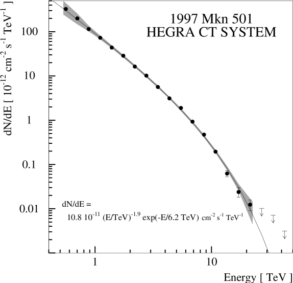
Figure 9: Time-averaged energy spectrum of Mrk 501 for the 1997 observation period. Vertical errors bars indicate statistical errors. The hatched area gives the estimated systematic errors, except the 15% uncertainty on the absolute energy scale. The lines shows the fit discussed in the text.

The spectrum shows a gradual steepening over the entire energy range. A fit of the data from 500 GeV to 24 TeV with a power law model with an exponential cut off gives:

$$dN/dE\,=\,N_{0}\,(E/1\,{\rm TeV})^{-\alpha}\,\exp{(-E/E_{0})}\leavevmode\nobreak\ \leavevmode\nobreak\ ,$$ (6)

$N_{0}=(10.8\leavevmode\nobreak\ \pm 0.2_{\rm stat}\leavevmode\nobreak\ \pm 2.1_{\rm sys})\cdot 10^{-11}\,\rm cm^{-2}s^{-1}TeV^{-1}$, $\alpha=1.92\leavevmode\nobreak\ \pm 0.03_{\rm stat}\leavevmode\nobreak\ \pm 0.20_{\rm sys}$, and $E_{0}=(6.2\leavevmode\nobreak\ \pm 0.4_{\rm stat}\leavevmode\nobreak\ (-1.5\leavevmode\nobreak\ +2.9)_{\rm sys})$ TeV. The systematic errors on the fit parameters result from worst case assumptions concerning the systematic errors of the data points, and their correlations and include the error caused by the 15% uncertainty in the energy scale. The errors on the fit parameters, especially on $\alpha$ and $E_{0}$, are strongly correlated. The variation of only one of the parameters within the quoted error range yields spectra which are inconsistent with the measured spectrum. The data points and their errors are summarized in Table 1.

Table 1: The time-averaged differential spectrum of Mkn 501

Ea	${\rm d}N/{\rm d}E$  b	$\sigma_{\rm stat}\leavevmode\nobreak\ \leavevmode\nobreak\ ^{c}$	$\sigma_{\rm sys}\leavevmode\nobreak\ \leavevmode\nobreak\ \leavevmode\nobreak\ ^{d}$
0.56	3.29 $10^{-10}$	1.68 $10^{-11}$	(+1.82 -1.07) $10^{-10}$
0.70	2.01 $10^{-10}$	7.45 $10^{-12}$	(+6.33 -4.75) $10^{-11}$
0.88	1.15 $10^{-10}$	3.45 $10^{-12}$	(+1.88 -1.68) $10^{-11}$
1.11	7.33 $10^{-11}$	1.88 $10^{-12}$	(+7.42 -7.08) $10^{-12}$
1.39	4.40 $10^{-11}$	1.10 $10^{-12}$	(+3.75 -3.45) $10^{-12}$
1.75	2.87 $10^{-11}$	7.25 $10^{-13}$	(+2.12 -1.97) $10^{-12}$
2.20	1.64 $10^{-11}$	4.64 $10^{-13}$	(+1.03 -0.97) $10^{-12}$
2.76	1.02 $10^{-11}$	3.14 $10^{-13}$	(+6.71 -6.30) $10^{-13}$
3.46	5.64 $10^{-12}$	1.98 $10^{-13}$	(+3.50 -3.30) $10^{-13}$
4.35	3.12 $10^{-12}$	1.27 $10^{-13}$	(+1.94 -1.83) $10^{-13}$
5.46	1.90 $10^{-12}$	8.73 $10^{-14}$	(+1.24 -1.16) $10^{-13}$
6.86	9.29 $10^{-13}$	5.24 $10^{-14}$	(+6.40 -5.99) $10^{-14}$
8.62	4.71 $10^{-13}$	3.28 $10^{-14}$	(+3.42 -3.19) $10^{-14}$
10.83	1.95 $10^{-13}$	1.82 $10^{-14}$	(+1.69 -1.56) $10^{-14}$
13.60	6.24 $10^{-14}$	1.02 $10^{-14}$	(+9.32 -8.11) $10^{-15}$
17.08	2.39 $10^{-14}$	5.85 $10^{-15}$	(+5.87 -4.71) $10^{-15}$
21.45	1.24 $10^{-14}$	3.35 $10^{-15}$	(+5.93 -4.01) $10^{-15}$
26.95	$<$ 1.0 $10^{-14}$ $\,{}^{e}$
33.85	$<$ 7.2 $10^{-15}$ $\,{}^{e}$
42.51	$<$ 3.1 $10^{-15}$ $\,{}^{e}$
a energy in TeV
b in (cm-2 s-1 TeV-1)
c statistical error in (cm-2 s-1 TeV-1)
d systematic error on the shape of the spectrum in
(cm-2 s-1 TeV-1)
e upper limits in (cm-2 s-1 TeV-1) at 2 $\sigma$ confidence level

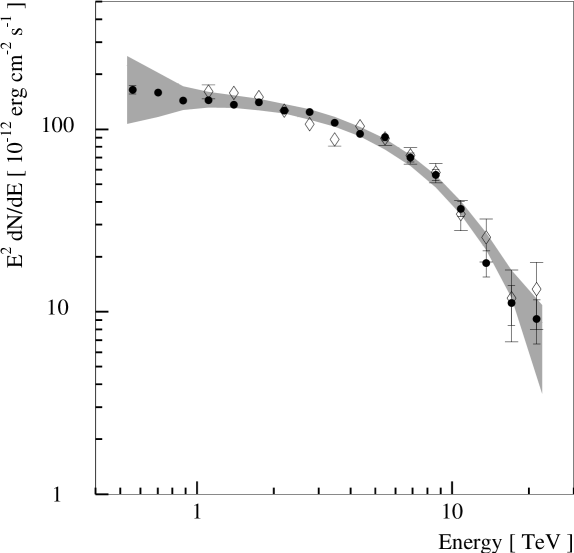
Figure 10: The spectral energy distribution $E^{2}\mbox{d}N/\mbox{d}E$, for the data set of low zenith angles ($\theta<30^{\circ}$, full circles) and for the data set of large zenith angles ($\theta$ between $30^{\circ}$ and 45^∘, 32 h observation time, open symbols). Since the observation periods do not overlap for the variable source, the spectra are normalized at the energy 2 TeV. The hatched band indicates the systematic error on the shape of the spectrum for the low zenith angle data. The systematic error on the high zenith angle spectrum at energy E approximately equals the systematic error on the low zenith angle spectrum at energy E/2.

Figure 11: The upper panel illustrates the spectral energy distribution $E^{2}\mbox{d}N/\mbox{d}E$, for the full data set (full circles), for periods of low flux (open circles), and for periods of high flux (triangles) ( dN/dE(2 TeV) above 30 and below 16 times $10^{-12}{\rm cm^{-1}s^{-1}TeV^{-1}}$). Only the statistical errors are given here; the systematic errors enter the three spectra in the same way and can be neglected comparing the three spectra. The dashed lines indicate the shape of the mean spectrum (fit from Eq. 6) overlaid over all three spectra to simplify the comparison of the shape of the three spectra. In the lower panel the ratio of the low flux spectrum divided by the high flux spectrum is shown. The dashed line gives the fit to a constant. The $\chi^{2}$-value is 12.3 for 15 degrees of freedom.

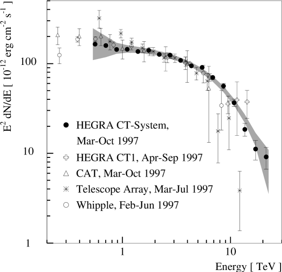
Figure 12: The Time-averaged spectrum of Mrk 501 during 1997, compared with published results from other experiments (Aharonian et al. 1999c , Hayashida et al. hay:98 (1998), Samuelson et al. samuel:98 (1998), Barrau et al. barr:97 (1998)). Since the observation periods do not completely overlap for the variable source, the spectra are normalized at the energy 2 TeV. For the HEGRA system the hatched area shows the systematic errors on the shape of the spectrum as described in the text. For the other experiments only statistical errors are shown. Only data points with a signal to noise ratio larger than one have been used.

In the highest energy bin (19 TeV to 24 TeV) 40 excess events are found above a background of 13 events, corresponding to a nominal significance of S = (N_on - N_off) / $\sqrt{\rm N_{on}+N_{off}}$ of 3.7 $\sigma$. However, due to the steep spectrum in this energy range, a part of these events may represent a spill-over from lower energies. To provide an absolutely reliable lower limit on the highest energies in the sample, the spectrum was fit to the form of Eq. 6, but with a sharp cutoff at $E=E_{cut}$: $dN/dE=N_{0}$ $(E/1\leavevmode\nobreak\ \rm TeV)^{-\alpha}$ $\exp{(-E/E_{0})}$ $\Theta(E_{cut}-E)$. The best fit is achieved with $E_{\rm cut}=28$ TeV; the $2\sigma$ lower limit is $E_{cut}=16$ TeV.

Fig.  10 illustrates the spectral energy distribution, $E^{2}dN/dE(E)$ as determined from the small zenith angle data ($<$30^∘, energy threshold 500 GeV) and the large zenith angle data (30^∘ to 45^∘, 32 h observation time, energy threshold 1 TeV). Note that the large zenith angle data has mainly been acquired during the second half of the 1997 data taking period. Nevertheless the shape of both spectra agrees within the statistical and systematic errors. The combined small and large zenith angle data set yields the same lower limit on $E_{cut}$ of 16 TeV as derived from the small zenith angle data alone. It can be recognized that the spectral energy distribution is essentially flat from 500 GeV up to $\simeq$ 2 TeV.

Figure  11 (upper panel) shows the spectral energy distribution for the overall data sample and for periods of high and low flux separately: dN/dE(2 TeV) determined on diurnal basis above 3 and below 1.6 $10^{-11}{\rm cm^{-1}s^{-1}TeV^{-1}}$, with a ratio of the mean fluxes close to 5. The high and low flux spectra agree within statistical errors, as shown by the ratio of both spectra, presented in Fig. 11 (lower panel). The systematic error is to good approximation the same for both data samples and cancels out in the ratio. The result thus confirms our previous conclusion about the flux-independence of the spectrum of Mkn 501 in 1997 between 1 and 10 TeV (Paper 1). Now the statement is extended to the broader energy region, from 500 GeV to 15 TeV. From 1 TeV to several TeV the slope of the spectrum is determined with high statistical accuracy, e.g. a power law fit in the energy region from 1 TeV to 5 TeV gives a differential index of -2.23 $\pm 0.04_{\rm stat}$ and -2.26 $\pm$0.06_stat for the high and the low flux spectrum respectively. In the narrow energy range from 500 GeV to 1 TeV the statistical uncertainty on the spectral index is considerably larger, we compute 0.2 for the high flux sample and 0.4 for the low flux sample. Therefore, our 1997 Mkn 501 data would not contradict a correlation of emission strength and spectral shape below 1 TeV as tentatively reported by the CAT-group (Djannati-Atai et al. CATcorrelation (1999)).

For completeness, the HEGRA IACT system data are plotted in Fig. 12 jointly with the HEGRA CT1 (Aharonian et al. 1999c ), the CAT (Barrau et al. barr:97 (1998)), the Telescope Array (Hayashida et al. hay:98 (1998)), and the Whipple (Samuelson et al. samuel:98 (1998)) results concerning the Mrk 501 energy spectrum during the 1997 outburst. Generally a good agreement can be recognized in the overlapping energy regions, except for a steeper Telescope Array spectrum.

6 Discussion

The observations of Mkn 501 by the HEGRA IACT system during the long outburst in 1997 convincingly demonstrate for the first time that the energy spectrum of the source extends well beyond 10 TeV. We believe that this very fact, together with the discovery of a time- and flux- independent stable spectral shape of the TeV radiation will have considerable impact on our understanding of the nonthermal processes in AGN jets.

This discussion is not an attempt at detailed modeling of the result presented in the previous section; this will be done elsewhere. Neither shall we systematically invoke multi-wavelength observations. Our purpose is rather to point out the multiple facets of the $\gamma$-ray  phenomenon on its own. They stem from the fact that the emission probably originates from a population of accelerated particles within a spatially confined relativistic jet, specifically oriented towards the observer, and that subsequently the radiation must propagate through the diffuse extragalactic background radiation field (DEBRA) before it reaches us. Each of these circumstances can influence the characteristics of the emitted spectrum, and we shall address them in turn below.

6.1 Production and absorption of TeV photons in the jet

The enormous apparent VHE $\gamma$-ray  luminosity of the source, reaching $\sim 10^{45}\,\rm erg/s$ during the strongest flares which typically last $\Delta t=\,1$ day or less, implies that the $\gamma$-rays  are most probably produced in a relativistic, small-scale (sub-parsec) jet which is directed along the observer’s line of sight. The determining quantity is the so-called Doppler factor $\delta_{\rm j}=[(1+z)\Gamma_{\rm j}(1-\beta_{\rm j}\cos{\Theta})]^{-1}$, where z is the redshift of a source moving with velocity $\beta_{\rm j}c$ and Lorentz factor $\Gamma_{\rm j}=(1-\beta_{\rm j}^{2})^{-1/2}$ along the jet axis that makes an angle $\Theta$ with the direction to the observer. Moreover, the assumption of relativistic bulk motion appears to be unavoidable in order to overcome the problem of severe $\gamma-\gamma$ absorption by pair production on low-frequency photons inside the source (see e.g. Dermer & Schlickeiser Der:94 (1994)). Indeed, assuming that the $\gamma$-radiation is emitted isotropically in the frame of a relativistically moving source, the optical depth at the observed $\gamma$-ray  energy is easily estimated as

$$\tau_{\gamma\gamma}\simeq\frac{f_{\rm r}d^{2}\sigma_{\rm T}\delta_{\rm j}^{-6}\,E}{8m_{\rm e}^{2}c^{6}\Delta t}\simeq 0.065f_{-10}\Delta t_{\rm day}^{-1}\delta_{10}^{-6}H_{60}^{-2}E_{\rm TeV}$$ (7)

Here $\delta_{10}=\delta_{\rm j}/10$, $\Delta t_{\rm day}=\Delta t/1\,\rm day$, $E_{\rm TeV}=E/1\,{\rm TeV}$, with $E$ the energy of the gamma-ray in the laboratory frame, and $f_{-10}=f_{\rm r}/10^{-10}\,\rm erg/cm^{2}s$ is the observed energy flux at $h\nu\simeq 100\delta_{10}^{2}\,E_{\rm TeV}^{-1}\,\rm eV$ which for an order of magnitude estimate is assumed to be constant at the optical to UV wavelengths that predominantly contribute to the $\gamma$-ray  absorption. Furthermore $d=cz/H_{0}=170H_{60}^{-1}$ Mpc is the distance to the source with redshift $z=0.034$, normalized to the value of the Hubble constant $H_{60}=H_{0}/60\,{\rm km/sMpc}$. Assuming now that the observed optical/UV flux of Mkn 501, $f_{-10}\simeq 0.5$ (see e.g. Pian et al. Pian:98 (1998)), is produced in the jet, the absorption of 20 TeV $\gamma$-rays  becomes negligible only when $\delta_{\rm j}\geq 10$; already for $\delta_{\rm j}=8$ internal absorption would be catastrophic for $\Delta t_{\rm day}=1$, with $e^{-\tau_{\gamma\gamma}}\leq 10^{-2}$. One may interpret the detected VHE spectrum of Mkn 501 given by Eq. 6 as a power-law production spectrum, modified by internal $\gamma-\gamma$ extinction with optical depth $\tau=E_{\rm TeV}/6.2$. This would give an accurate determination of the jet’s Doppler factor taking into account the very weak dependence of $\delta_{\rm j}$ on all relevant parameters, namely $\delta_{\rm j}=8.5\,f_{-10}^{1/6}\Delta t_{\rm day}^{-1/6}\,H_{60}^{-1/3}$. Since there could be a number of other reasons for the steepening of the TeV spectrum, that estimate can only be considered as a robust lower limit on $\delta_{\rm j}$.

The strong steepening of the observed spectrum of Mkn 501 above several TeV could also be attributed, for example, to an exponential cutoff in the spectrum of accelerated particles. These could either be protons producing $\gamma$-rays  through inelastic $p-p$ interactions and subsequent $\pi^{0}$-decay , or electrons producing $\gamma$-rays  via inverse Compton (IC) scattering. In IC models an additional steepening of the $\gamma$-ray  spectrum is naturally expected due to the production of TeV $\gamma$-rays  in the Klein-Nishina regime if the energy losses of electrons are dominated by synchrotron radiation in the jet’s magnetic field. And finally, the exponential cutoff in the observed TeV spectrum could be caused by $\gamma$-$\gamma$ absorption of TeV photons in a possible dust torus surrounding the AGN (Protheroe & Biermann PrBr:96 (1996)) and in the extragalactic diffuse background radiation (Nikishov Nik:62 (1962), Gould & Schreder Gould:65 (1965), Jelly Jelly:65 (1965), Stecker et al. Steck:92 (1992)).

Our current poor knowledge about the distortion of the source spectrum caused by internal and intergalactic absorption does not allow us to distinguish between hadronic and leptonic source models on the basis of their predictions concerning the TeV energy spectra. Fortunately the temporal characteristics are to a large extent free from these uncertainties. Thus we believe that real progress in this area can only be achieved by the analysis of both the spectral and temporal characteristics of X-ray and TeV $\gamma$-ray  emissions obtained during multiwavelength campaigns that investigate several X-ray selected BL Lac objects in different states of activity, and located at different distances within several 100 Mpc. Notwithstanding this belief, we show here that the high-quality HEGRA spectrum of Mkn 501 alone allows us to make quite a few interesting inferences about the $\gamma$-ray  production and absorption mechanisms.

6.1.1 IC models of the gamma ray emission.

Currently it is believed (e.g. Ulrich et al. umu:97 (1997)) that the correlated X-ray/TeV flares discovered by multiwavelength observations of Mkn 421 (Takahashi et al. tak:96 (1996), Buckley et al. buk:96 (1996)) and Mkn 501 (Catanese et al. cat:97 (1997), Pian et al. Pian:98 (1998), Paper 1), support the hypothesis of both emission components originating in relativistic jets due to synchrotron/IC radiation of the same population of directly accelerated electrons (Ghisellini et al. GhisMD:1996 (1996); Bloom & Marscher BlMar:96 (1996); Inoue & Takahara IT:1996 (1996); Mastichiadis & Kirk Mast:97 (1997); Bednarek & Protheroe BedPro:97 (1997)). One of the distinctive features of leptonic models is that they allow significant temporal and spectral variations of TeV radiation. The stable shape of the TeV spectrum of Mkn 501 during the 1997 outburst does not contradict these models. It rather requires them to have two important features.

First of all the form of the spectrum of accelerated electrons should be essentially stable in time and be independent of the strength of the flare up to electron energies responsible for the production of the highest observed $\gamma$-ray  energies $E\geq 16{\rm TeV}$. For a typical Doppler factor $\delta_{\rm j}\sim 10$ this implies relatively modest electron energies $E_{\rm e}\leq 10\,{\rm TeV}$ in the jet frame, assuming that the Compton scattering at the highest energies takes place in the Klein-Nishina limit. In this limit a significant fraction of the electron energy goes to the upscattered photon, i. e. $E\sim\delta_{\rm j}\,E_{\rm e}$.

For low values of the magnetic field in the emitting plasma, i.e. B $\stackrel{{\scriptstyle<}}{{\scriptstyle\sim}}$ 0.01 G, the X-ray spectrum could be more sensitive to accelerated electrons with energies above 10 TeV. The typical observed energy of X-rays produced by electrons of energy $E_{\rm e}$ in the jet frame is

$$E_{\rm X}\simeq 20(B/0.1\,{\rm G})\,(E_{\rm e}/1\,{\rm TeV})^{2}\,\delta_{10}\,{\rm keV}.$$ (8)

The BeppoSAX observations of Mkn 501 in April 1997 showed that the X-ray spectrum becomes very hard during strong flares. This is interpreted as a shift of the synchrotron peak to energies in excess of 100 keV (Pian et al. Pian:98 (1998)). Formally this effect could be explained by a significant increase in each of the three parameters which determine the position of the synchrotron peak, i.e. the maximum electron energy $E_{{\rm e},max}$, the magnetic field $B$, and the jet Doppler factor $\delta_{\rm j}$.

The rather stable energy spectrum of TeV radiation implies that the spectrum of the parent electrons does not significantly vary during the HEGRA observations, the latter performed with typical integration times between one and two hours. The condition of a constant acceleration spectrum does not yet guarantee a stable energy spectrum of TeV radiation. Therefore we need a second condition, namely to assume very effective radiative (synchrotron and IC) cooling of electrons, sufficiently fast to establish an equilibrium electron spectrum within $\Delta t^{\ast}=10\,\delta_{10}\,\rm h$. The radiative cooling time is

$$t_{\rm rad}=(\frac{4}{3}\,\sigma_{\rm T}\,c\,w_{0}\,E_{\rm e}/m_{\rm e}c^{2})^{-1}\simeq$$ (9)

$$\hskip 22.76228pt\simeq 15.5\,(w_{0}/1\,{\rm erg/cm^{3})^{-1}}\,E_{\rm TeV}\,\rm s,$$

where $w_{0}=B^{2}/8\pi+w_{\rm r}$ is the total energy density of magnetic and photon fields. Thus, for a jet magnetic field of about $0.1\,\rm G$ and a comparable low-frequency photon density ($\approx 4\cdot 10^{-4}\,\rm erg/cm^{3}$) a radiative cooling time of less than 5 hours (in the jet frame) could be easily achieved.

6.1.2 $\pi^{0}$ origin of gamma rays

The lack of correlation between spectral shape and absolute flux, as well as the very fact that $\gamma$-rays  with energy $\geq 16\,\rm TeV$ are observed, could also be explained, perhaps even in a more natural way, by the assumption of a ‘$\pi^{0}$-decay’ origin of the $\gamma$ -radiation. Yet the efficiency of this mechanism in the jet appears to be too low to explain the observed time variability and the high fluxes of the TeV radiation. This is due to the low density $n_{\rm H}$ of the thermal electron-proton plasma in the jet. The problem of variability could be at least in principle overcome by invoking adiabatic losses caused by relativistic expansion of the emitting “blob”. However, this assumption implies very inefficient $\gamma$-ray  production with a luminosity $L_{\gamma}=L_{p}t_{\rm ad}/t_{\rm pp}^{\pi^{0}}$, where $L_{\rm p}$ is the luminosity in relativistic protons, $t_{\rm ad}\geq R/c\sim\Delta t\delta{\rm j}$ is the adiabatic cooling time, and $t_{\rm pp}^{\pi^{0}}\sim 5\cdot 10^{15}(n_{\rm H}/1{\rm cm}^{-3})^{-1}\,s$ denotes the characteristic emission time scale of $\pi^{0}$-decay $\gamma$-rays. We shall assume here that the proton luminosity $L_{\rm p}$ should not exceed the total power of the central engine, roughly the Eddington luminosity $L_{\rm E}=1.3\cdot 10^{45}\,(M/M_{\odot})\,\rm erg/s$ of a supermassive Black Hole of mass $M=10^{7}M_{\odot}$, or more empirically, the apparent ($4\pi$) total luminosity of the source which is $L_{\rm tot}=4\cdot{\pi}d^{2}\cdot f_{\rm tot}\sim 10^{45}$ erg/s, where $f_{\rm tot}\sim{\rm few}\times 10^{-10}\,\rm erg/cm^{2}s$ is the total observed radiative flux (see e.g. Pian et al. Pian:98 (1998)). Then the observed TeV-flux of about $2.5\cdot 10^{-10}$ erg/s requires a lower limit $n_{\rm H}\geq 10^{6}{\rm cm}^{-3}$ on the density of the thermal plasma in the jet. This makes the relativistically moving ‘blob’ very heavy ($M\sim 0.05M_{\odot}$) with an unacceptably large kinetic energy $E_{\rm kin}=Mc^{2}\Gamma_{\rm j}\simeq 10^{54}\Delta t_{\rm day}^{3}\delta_{10}^{4}(n/10^{6}\,\rm cm^{-3})$ erg.

We would like to emphasize that these arguments hold against the $\pi^{0}$-origin of $\gamma$-rays  produced in a small-scale jet; they do not in general exclude hadronic models. In particular, scenarios like the one assuming $\gamma$-radiation produced by gas clouds that move across the jet (Bednarek & Protheroe BedPro:97 (1997)), Dar & Laor dar:97 (1997)) remain an attractive possibility for hadronic models. They do not exclude either a “proton blazar” model (Mannheim Man:93 (1993)). It implies a secondary origin of the relativistic electrons that are the result of electromagnetic cascade, triggered by photo-meson processes involving extremely high energy protons in a hadronic jet (see Mannheim Man:98 (1998) and references therein).

6.2 Intergalactic extinction

The effect of intergalactic extinction of VHE $\gamma$-rays  in diffuse extragalactic background radiation fields became astrophysically significant (see e.g. Stanev & Franceschini Stanev:98 (1998), Funk et al. Magn:97 (1998), Biller et al. Bill:98 (1998), Stecker & de Jager Stec:98 (1998), Biller vbill:98 (1998), Primack et al. vprim:98 (1998), Stecker vsteck:98 (1998)) after the discovery of TeV radiation from Mkn 421 and Mkn 501 up to energies of 10 TeV, as reported by the Whipple (Zweerink et al. Zv:97 (1997)), and HEGRA (Aharonian et al. 1997a), CAT (Djannati-Atai et al. CATcorrelation (1999)), and Telescope Array (Hayashida et al. hay:98 (1998)) groups.

6.2.1 Gamma ray absorption

If we ignore the appearance of second generation $\gamma$-rays (see Sect. 6.2.2), then extinction is reduced to a simple absorption effect which can be described by a single absorption optical depth $\tau$.

The optical depth $\tau$ of the intergalactic medium for a $\gamma$-ray photon of energy $E$, emitted from a source at the distance $d=cz/H_{0}$, can be expressed for small redshifts z$\ll$ 1 in a convenient approximate form using a quantity $\tau=\tau^{\prime}\xi$, where

$$\tau^{\prime}(E)=\frac{\sigma_{\rm T}}{4}\,\epsilon_{\rm m}n(\epsilon_{\rm m})\,d\simeq$$ (10)

$$\hskip 14.22636pt0.08\left(\frac{\epsilon_{\rm m}^{2}n(\epsilon_{\rm m})}{10^{-3}\,\rm eV/cm^{3})}\right)\,\left(\frac{z}{0.034}\right)E_{\rm TeV}\,H_{\rm 60}^{-1}$$

with $H_{\rm 60}=H_{0}/60\,\rm km/s\,Mpc$, $E_{\rm TeV}=E/1\,\rm TeV$, $\epsilon_{\rm m}=4m^{2}_{\rm e}c^{4}/E\simeq 1E_{\rm TeV}^{-1}\,\rm eV$, and $\xi$ being a correction factor which accounts for the specific form of the differential DEBRA photon number density $n(\epsilon)$; the background photon energy is denoted by $\epsilon$. This expression is based on the narrowness of the $\gamma\gamma\rightarrow e^{+}e^{-}$ cross-section $\sigma_{\gamma\gamma}$ as a function of $(\epsilon/\epsilon_{\rm m})$ which peaks at $\epsilon/\epsilon_{\rm m}\simeq 1$ in an isotropic field of background photons (Herterich her:74 (1974)). Thus for a large class of broad DEBRA spectra $n(\epsilon)$ the optical depth is essentially caused by background photons with energy centered around $\epsilon_{\rm m}$. For (broad) power-law spectra, $n(\epsilon)=n_{0}\epsilon^{-\gamma}$, the optical depth can be calculated analytically as $\tau(E)=\eta(\gamma)\cdot 4^{\gamma}(\sigma_{\rm T}/4)\epsilon_{\rm m}n(\epsilon_{\rm m})\,d$, where $\eta(\gamma)=7/6\gamma^{-5/3}(1+\gamma)^{-1}$ (Svensson sven:87 (1987)). Thus for relatively flat power-law spectra with $1<\gamma<2.5$ we obtain $\xi=4^{\gamma}\eta(\gamma)\simeq 2$, i.e. approximately half of $\tau_{\gamma\gamma}$ is contributed by background photons with $\epsilon$ in the interval given by $\epsilon_{\rm m}\pm 1/2\epsilon_{\rm m}$.

Figure 13: The energy fluxes of DEBRA for pure power-law differential spectra with $\gamma=1$ (curve 1), $\gamma=2$ (curve 2) and $\gamma=3$ (curve 3). Curve 4 is the sum of spectra 1 and 3. The absolute flux normalizations have been determined from the condition of $\tau_{\gamma\gamma}=3$ (for curve 1), and from the condition of the maximum possible flux of DEBRA which still “reproduce” reasonable $\gamma$-ray  source spectra shown in Fig.  14 (for curves 2 and 3). The horizontal bars correspond to the upper limits on DEBRA fluxes obtained using a method similar to the one suggested by Biller et al. (1998). The curve marked as “MBR” correspond to the density of the 2.7 K MBR. The tentative flux measurement at 3.5 $\mu$m is taken from Dwek & Arendt (1998), and the flux estimates based on the ISO survey at 6 and 15 $\mu$m are from Stanev & Franceschini (1998). The other measured fluxes and the upper/lower limit estimates of the DEBRA are taken from the recent compilation by Dwek et al. (1998), i.e., the upper limit at 2.2 $\mu$m is from Hauser et al. (1998), the lower limit at 2.2 $\mu$m is from Gardner et al. (1997), and the UV to optical detections are from Pozzetti et al. (Poz:98 (1998)).

We note that $\tau(E)\propto E^{\gamma-1}$ for a power-law spectrum of DEBRA . For example, within the ‘valley’ of the energy density at mid infrared wavelengths from several $\mu\rm m$ to several tens of $\mu\rm m$, where the energy density is expected to be more or less constant (i.e. $\epsilon^{2}n(\epsilon)={\rm const}$), the intergalactic extinction of $\gamma$-rays  is largest at the highest observed energies. In particular, according to Eq. 10, even at a very low and probably unrealistic level of the DEBRA intensity of $\epsilon^{2}n(\epsilon)=10^{-4}\,\rm eV/cm^{3}$ at $\lambda\sim 30\,\rm\mu m$, approximately $35\,\rm percent$ of the 25 TeV $\gamma$-rays emitted by Mkn 501 are extinguished before they reach the observer. This implies that the observed TeV spectrum of Mkn 501 contains important information about the DEBRA, at least at wavelengths $\lambda\geq 10\mu\rm m$. Moreover, it is quite possible that a non-negligible intergalactic extinction takes place also at low $\gamma$-ray  energies due to interactions with near infrared (NIR) background photons. Interpreting the power-law shape of the spectrum at $2\,\rm TeV$ as an indication for weak extinction by, say, a factor less than or equal to 2, and ignoring the contributions from all other wavelengths beyond the interval $0.5\pm 0.25\,\rm eV$ ($\lambda\simeq 2.5^{\rm+2.5}_{\rm-0.85}\,\,\mu\rm m$) from Eq. 10, one obtains $\epsilon^{2}n(\epsilon)\leq 4\times 10^{-3}\,H_{\rm 60}\;\rm eV/cm^{3}$, not far from the flux of DEBRA experimentally inferred (Dwek et al. dwek:98 (1998), de Jager & Dwek gt:98 (1998)) and theoretically expected (Malkan & Stecker malk:98 (1998), Primack et al. vprim:98 (1998)) at these wavelengths.

However, to the extent that the source spectrum of the $\gamma$-rays  is unknown, this cannot be considered as a model-independent upper limit (e.g. Weekes et al. GRO4rev:97 (1997)). Obviously for any quantitative estimate of the DEBRA one needs to know the intrinsic $\gamma$-ray  spectrum, and this can not be obtained from $\gamma$-ray  observations alone. As already emphasized above, a multi-wavelength approach is indispensable, for example in the form of detailed modeling of the entire or at least a large wave-length range of the nonthermal spectrum. To be specific, one avenue would be modeling the nonthermal X-ray and $\gamma$-ray  spectra in the framework of synchrotron-inverse Compton models, based on simultaneous multi-wavelength observations of X-ray selected BL Lac objects (Coppi & Aharonian CoAh:98 (1999)).

Figure 14: The source spectra of Mkn 501 reconstructed for different models of DEBRA. The heavy dots correspond to the measured spectrum of HEGRA approximated by Eq. 6 with $\gamma=1.92$, and $E_{0}=6.2\,\rm TeV$. The curves 1, 2, and 3 correspond to the power-law DEBRA spectra shown in Fig. 13 by curves 1,2 and 3, respectively. The vertical line at 16 TeV indicates the edge of the $\gamma$-ray  spectrum of Mkn 501 measured by HEGRA.

An illustration for the need of more than $\gamma$-ray  data alone is given by a DEBRA spectrum $n(\epsilon)\propto\epsilon^{-1}$. It does not change the spectral shape of $\gamma$-rays  at all (grey opacity), although formally the extinction could be arbitrarily large. The curves marked as “1” in Fig. 13 and Fig. 14 may serve as an example. In the case of Mkn 501 this ambiguity can be significantly reduced by rather general arguments regarding $\gamma$-ray energetics. Requiring again that the $\gamma$-ray  luminosity should not exceed the total apparent luminosity of the source, $L_{tot}\sim 10^{45}\,\rm erg/s$, we must have $\rm e^{\tau}\leq 10^{4}(\delta_{\rm j}/10)^{4}$. For $\gamma$-ray  production in the jet with $\delta_{\rm j}\sim 10$, this implies $\tau\leq 10$. In fact, already a value of $\tau\sim 3$ (corresponding to curve 1 of Fig. 13) creates uncomfortable conditions for the majority of realistic models of high energy radiation from Mrk 501, assuming that the nonthermal emission is produced in the jet due to synchrotron and inverse Compton processes. Indeed, $\tau_{\gamma\gamma}\sim 3$ implies that the $\gamma$-ray luminosity of the source corresponding to the “reconstructed spectrum” (curve 1 in Fig. 14) exceeds the luminosity of the source in all other wavelengths by an order of magnitude which hardly could be accepted for any realistic combination of parameters characterizing the jet.

Accepting the current lack of reliable knowledge of the $\gamma$-ray  source spectrum, it is nevertheless worthwhile to derive upper limits on DEBRA by formulating different a priori, but astrophysically meaningful requirements on the spectrum and the $\gamma$-ray  luminosity of the source. A possible criterion, for example, could be that within any reasonable source model the intrinsic spectrum of $\gamma$-rays, $J_{0}(E)=J_{\rm obs}\,\exp(\tau)$, should not contain a feature which exponentially rises with energy at any observed $\gamma$-ray  energy. In practice this implies that the ‘reconstruction’ factor $\exp(\tau)$ should not significantly exceed the exponential term of the observed $\gamma$-ray  spectrum from Eq. 6. This condition is most directly fulfilled by the power law-spectrum with $\gamma=2$ that has equal DEBRA power per unit logarithmic bandwidth in energy. It results in $\tau(E)\propto E$ and then yields an upper limit for the DEBRA density close to $\epsilon^{2}n(\epsilon)=10^{-3}\rm eV/cm^{3}$. This limit corresponds to the borderline on which the source spectrum becomes a pure power-law Figs. 13 and 14, curves 2. A slight increase of the DEBRA density by as little as a factor of 1.5 leads to a dramatic (exponential) deviation of the reconstructed spectrum at the highest observed $\gamma$-ray  energies around 16 TeV from the $E^{-1.9}$ power-law extrapolation.

A power law with $\gamma=3$ would give similar and complementary results. The resulting source spectra (Fig. 14) and the upper limits on the DEBRA density (Fig. 13) obtained in this way assuming power-law spectra for DEBRA with $\gamma=2$ and 3, are given by the curves 2 and 3, respectively. The power law $\gamma=1$ corresponding to $\tau_{\gamma\gamma}=3$ complements Fig. 13.

Figure 15: The same as in Fig. 13, but for different parameters of the power-law DEBRA. Curve 1: $\gamma=1$ with an absolute flux corresponding to $\tau_{\gamma\gamma}=1$; curve 2: $\gamma=1$ with $\epsilon^{2}n(\epsilon)=3\cdot 10^{-4}\,\rm eV/cm^{3}$; curve 3: $\gamma=4$; curve 4: sum of spectra 1 and 3, truncated at 1 and 80 $\mu$m.

It should be noted however that any realistically expected spectrum of the DEBRA in a broad range of wavelengths deviates from a simple power-law. In fact, all models of the DEBRA, independently of the details, predict two pronounced peaks in the spectrum at 1 $\mu$m and 100 $\mu$m contributed by the emission of the stars and of the interstellar dust, respectively, and a relatively flat ‘valley’ at mid IR wavelengths around 10 $\mu$m (see e.g. Dwek et al. dwek:98 (1998)). The strong impact of the DEBRA spectrum on calculations of the opacity of the intergalactic medium has been emphasized by Dwek & Slavin (DwSl:1994 (1994)) and Macminn and Primack (Pri:96 (1996)).

Figure 16: The same as Fig. 14 but for DEBRA fluxes shown in Fig. 15, with the addition of a reconstructed spectrum (curve 4) corresponding to curve 4 in Fig. 15.

Note that the power law with $\gamma\sim 1$ characterizes the shape of the spectrum of DEBRA at near IR wavelengths, typically between 1 and several microns, and the power-law with $\gamma\geq 3$ characterizes the DEBRA between 10 and 100 microns. Interestingly, the sum of these two power law spectra “reproduces” a reasonable shape of the ‘valley’. This is seen in Fig. 13 and Fig. 15 where the measured fluxes or estimated upper and lower limits obtained directly at different wavelengths of the DEBRA are shown.

Finally, an interesting numerical criterion for the derivation of upper limits on the DEBRA was suggested by Biller et al. (Bill:98 (1998)). It relies on independent $\gamma$-ray observations. A variant of this approach, where the additional restriction forbids a differential source spectrum harder than $\propto E^{-1.5}$ within the observed energy range, is shown by the horizontal bars in Fig. 13.

The results described above could be “improved” assuming a more realistic, $\tau_{\gamma\gamma}=1$ optical depth for the $\gamma=1$ power law branch at short wavelengths, and a steeper, $\gamma=4$, power law branch at long wavelengths (see Fig. 15). The latter choice for $\gamma$ is due to the rapid rise of the data points towards far infrared wavelengths $\lambda$ in order to fit the recent measurements of the flux at $140\,\mu\rm m$ by DIRBE aboard the COBE satellite. For the far infrared (FIR) branch the absolute flux of the power-law with $\gamma=4$ is chosen again from the condition that the differential $\gamma$-ray source spectrum should not exponentially rise at energies up to $E\sim 16\,\rm TeV$ (see Fig. 16). Note also that the criterion of $\tau_{\gamma\gamma}=1$ for the $\gamma=1$ branch at short wavelengths is pretty close to the level of the flux of the recent tentative detection of DEBRA at $3.5\,\mu\rm m$ (Dwek & Arendt DwAr:98 (1998)). The sum of the NIR and FIR power-law branches with the above indices and absolute fluxes results in a deeper mid IR “valley” and predicts a very steep spectrum of DEBRA between 30 and 100 $\mu\rm m$. In Figs. 15 and 16 this spectrum has been truncated at $\lambda\simeq 80\mu\rm m$ that corresponds to the kinematic threshold of pair production at interactions with the maximum observed energy of $\gamma$-rays  of about 20 TeV. The spectrum is also truncated at $\lambda=1\mu\rm m$ in order to avoid significant excess compared with the fluxes at optical/UV wavelengths recently derived from the Hubble Deep Field analysis (Pozzetti et al. Poz:98 (1998)).

The effect of “reconstruction” of the $\gamma$-ray  spectra of Mkn 501 corresponding to this “best estimate” of DEBRA between 1 and 80 $\mu$m is illustrated in Fig. 16. It shows, in the simple absorption picture (using two truncated power-laws) that even a conservative choice for the DEBRA field implies intergalactic extinction at all observed energies. Especially the reconstructed spectrum around 1 TeV could be considerably harder than the observed spectrum, with a maximum of $E^{2}\,{\rm d}N/{\rm d}E$ at 2 TeV (see Fig. 9). This also demonstrates that it would be dangerous to interpret the observed spectral slope at low energies in terms of a power law extending from still lower energies.

6.2.2 The effect of cascading in the DEBRA

The discussion of intergalactic $\gamma-\gamma$ absorption effects is in principle incomplete without considering secondary radiations. Briefly, when a $\gamma$-ray  is absorbed by pair production, its energy is not lost. The secondary electron-positron pairs create new $\gamma$-rays  via inverse Compton scattering on the 2.7 K MBR. The new $\gamma$-rays  produce more pairs, and thus an electromagnetic cascade develops (Berezinsky et al. Berez:90 (1990), Protheroe & Stanev Prostan:93 (1993), Aharonian et al. AhCo:94 (1994)). In fact, in our discussion of absorption we have neglected any secondary $\gamma$-rays  in the field of view of the detector and we finally turn now to these.

For a primary $\gamma$-ray  spectrum ${\rm d}N/{\rm d}E$ harder than $E^{-2}$, extending to energies $E\gg 1{\rm TeV}$, the cascade spectrum at TeV energies could strongly dominate over the primary $\gamma$-ray  spectrum. In addition, the spectrum of the cascade $\gamma$-rays  that reach the observer has a standard form independent of the primary source spectrum with a characteristic photon index of $1.8-2.0$ at energies between $\sim 100\leavevmode\nobreak\ \rm GeV$ and an exponential cutoff determined by the condition $\tau(d,E)=1$. Thus, somewhat surprisingly, the measured time-averaged spectrum of Mkn 501 can in principle be fitted by a cascade $\gamma$-ray  spectrum for a reasonable DEBRA flux level of about $10^{-3}\,\rm eV/cm^{3}$, provided that the invisible source spectrum extends well beyond 25 TeV, say up to 100 TeV.

For an intergalactic magnetic field (IGMF) $B>10^{-12}\,\rm G$ the cascade $\gamma$-rays  could be observed in the form of an extended emission from a giant pair halo with a radius up to several degrees formed around the central source (Aharonian et al. AhCo:94 (1994)). Although the possible extinction of $\gamma$-rays  from Mkn 501, at least above 10 TeV, unavoidably implies the formation of a pair halo, the TeV radiation of Mkn 501 cannot be attributed to such a halo simply due to arguments based on the detected angular size and the time variability of the radiation.

However, the speculative assumption of an extremely low IGMF still allows an interpretation of the observed TeV $\gamma$-rays  of Mkn 501 within the hypothesis of a cascade origin. Instead of extended and persistent halo radiation, we expect in this case that the cascade $\gamma$-rays  penetrate from the source to the observer almost on a straight line. Yet at cosmological distances to the source even very small deflections of the cascade electrons by the IGMF lead to significant time delays of the arriving $\gamma$-rays: $\Delta t_{\rm B}\simeq 2.4(d/1\,{\rm Gpc})(E/1\,{\rm TeV})^{-2}(B/10^{-18}\,{\rm G})^{2}\,\rm days$ (Plaga Plaga:95 (1995)). This implies that in order to see more or less synchronous activity (within several days or less) of Mkn 501 at different wavelengths, as was observed during multiwavelength observations of the source (see e.g. Pian et al. Pian:98 (1998)), we would have to require $B\leq 10^{-18}\,\rm G$. Although indeed quite speculative, such small magnetic fields on spatial scales large compared to 1 Mpc cannot be a priori excluded (e.g. Kronberg Kron:96 (1996)).

7 Conclusions

In this paper we have presented the 1997 Mkn 501 time averaged spectrum as measured with the HEGRA IACT system in the energy range from 500 GeV to 24 TeV. The absence of strong temporal evolution as well as a significant correlation of the emission strength and the spectral shape in the energy region from 500 GeV to 15 TeV made the determination of a time averaged spectrum astrophysically meaningful. Due to unprecedented $\gamma$-ray  statistics and the 20% energy resolution of the instrument, it was possible to detect for the first time $\gamma$-rays from an extragalactic source with energies well beyond 10 TeV, and to measure a smooth, curved energy spectrum deeply into the exponential regime. We found, that the spectrum above 0.5 TeV is well described by a power law with an exponential cutoff $dN/dE$ = $\,N_{0}\,E^{-1.92}\,\exp{(-E/6.2\,\rm TeV)}$, the highest recorded photon energies being 16 TeV or more.

The detection of TeV $\gamma$-rays from Mkn 501 leads to the unavoidable conclusion that the observed $\gamma$-radiation is produced in a relativistic jet with a Doppler factor $\delta_{\rm j}\geq 10$. Actually, assuming a pure power-law production spectrum of $\gamma$-rays we may naturally explain the exponential cutoff in the observed spectrum spectrum by an internal $\gamma$-$\gamma$ absorption in the jet. Because of the strong dependence of the optical depth on the jet’s Doppler factor, this hypothesis gives an accurate determination of the latter, $\delta_{\rm j}=8.5$. Remarkably, the uncertainty of this estimate, which is mainly due to the uncertainty in the value of the Hubble constant, $H_{0}\simeq 60^{+40}_{-20}\,\rm km/cMpc$ and in the measured energy of the exponential cutoff $E_{0}=6.2\,\rm TeV$, does not exceed $20\%$. However, since there could be other reasons for the steepening of the TeV spectrum, this estimate can only be considered as a robust lower limit on $\delta_{\rm j}$. In particular, the steepening of the $\gamma$-ray spectrum at the highest energies could be attributed to an exponential cutoff in the spectrum of accelerated particles, as well as – in the case of the inverse Compton origin of $\gamma$-rays – to the Klein-Nishina effect.

In addition, a modification of the intrinsic (source) spectrum of TeV $\gamma$-rays takes place during their passage through the intergalactic medium. The recent claims about tentative detections of the diffuse extragalactic background radiation by the DIRBE instrument aboard the COBE at near infrared ($\lambda=3.5\mu\rm m$) and far infrared ($\lambda=140\mu\rm m$) wavelengths, both at the $\simeq 10\,\rm nW/cm^{2}sr$ flux level imply a strong effect of intergalactic $\gamma$-$\gamma$ extinction on the observed Mkn 501 spectrum over the entire energy region measured by HEGRA. In particular, the shape of the highest energy part of the observed $\gamma$-ray spectrum combined with the DIRBE flux at $140\mu\rm m$ requires a very steep ($\nu F_{\nu}\propto\lambda^{s}$ with $\nu\sim 4$) spectrum of the DEBRA with a characteristic flux at mid infrared wavelengths ($\lambda\sim 10-30\mu\rm m$) around 1 to 2 $\rm nW/m^{2}ster$. Due to the expected flat spectrum of DEBRA at near infrared wavelengths (close to $\nu F_{\nu}\propto\lambda^{-1}$) the modification of the $\gamma$-ray spectrum is less prominent at energies of a few TeV, although the absolute extinction could be very large. This does not allow us to draw definite conclusions about the absorption effect based on the analysis of the shape of the $\gamma$-ray spectrum. Nevertheless, in the case of Mkn 501 this ambiguity can be significantly reduced by rather general arguments regarding the $\gamma$-ray energetics. Indeed, even relatively modest assumption about the optical depth of about $\tau\sim 3$ which corresponds to a flux of the DEBRA in the K-band ($\lambda=2.2\mu\rm m$) of about $30\rm\,nW/m^{2}ster$ creates uncomfortable conditions for any realistic models of the high energy radiation from Mrk 501. Thus, this value of the flux of the DEBRA may be considered as a rather strong upper limit comparable with the DIRBE upper limit at this wavelength.

To summarize, our excursion through the nonthermal physics of AGNs shows that $\gamma$-ray  observations alone do not allow a unique interpretation of a spectrum like the one we have presented for Mkn 501, even though one can make a number of highly interesting inferences. In particular, our current poor knowledge about the intrinsic spectrum of Mkn 501 does not allow us to make definite conclusions about the effect of the intergalactic absorption of TeV $\gamma$-rays. And vice versa, the uncertainty in the density of DEBRA does not allow us to take into account the effect of the intergalactic absorption, and thus to “reconstruct” the intrinsic $\gamma$-ray spectrum. The knowledge of the latter is an obvious condition for the quantitative study of the acceleration and radiation processes in the source. Therefore we believe that decisive progress in this field could be achieved by the analysis of both the spectral and temporal characteristics of X-ray and TeV $\gamma$-ray emissions obtained during the multiwavelength campaigns of several X-ray selected BL Lac objects at different states of activity, and located at different distances within 1 Gpc. Due to the time variability of such sources this requires simultaneous observations together with extensive theoretical modeling. Given these we expect to obtain independent knowledge of the diffuse intergalactic radiation fields which can be compared with direct measurements and models of galaxy formation. We hope that the successful multiwavelength campaigns of Mkn 421 and Mkn 501 in 1998 with participation of several X-ray satellites and the HEGRA IACT system will provide highly interesting results in this area.

Acknowledgments. The support of the German ministry for Research and technology BMBF and of the Spanish Research Council CYCIT is gratefully acknowledged. We thank the Instituto de Astrophysica de Canarias for the use of the site and for supplying excellent working conditions at La Palma. We gratefully acknowledge the technical support staff of the Heidelberg, Kiel, Munich, and Yerevan Institutes.

Appendix A Systematic errors on the shape of the spectrum

To illustrate the effect of systematic errors for determination of energies and effective areas in more detail, we consider here the following model. For simplicity, we consider a detector consisting of a single Cherenkov telescope, which is located inside a uniformly illuminated Cherenkov light pool of area $A_{\rm pool}$. To good approximation, the light yield $I$ (in photons per m²) is proportional to the shower energy,

$$I=\alpha E$$ (11)

neglecting logarithmic corrections. The response of the telescope is now characterized by two quantities, namely the total intensity $Q$ detected in the image (usually the size, measured e.g. in units of ADC channels, or, with a conversion factor, in units of ‘photoelectrons’), and the signal $V$ induced in the highest pixel(s), which is fed into the trigger circuitry. Both $Q$ and $V$ should be proportional to $I$,

$$Q=\beta I\,;\,V=\gamma I\,,$$ (12)

but they are influenced by rather different factors. While both $\beta$ and $\gamma$ include the mirror reflectivity, the PMT quantum efficiency, and the PMT gain, $V$ is to a much higher degree sensitive to the point spread function of the mirror, and to the shape of the signal generated by the PMT . The effective detection area is given by

$$A=P(V)A_{\rm pool}$$ (13)

where $P$ is the trigger probability for a given value of $V$. The fact that triggering and energy determination are not based on identical quantities is the key origin of systematic errors, in particular in the threshold region.

In the analysis of data, values $\alpha_{\rm MC}$, $\beta_{\rm MC}$ and $\gamma_{\rm MC}$ are assumed for these constants, usually based on Monte Carlo simulations. The values may differ from the true values due to imperfections in the parameterization of the atmosphere ($\alpha$) or of the optics and electronics of the telescope ($\beta$, $\gamma$). The reconstructed energy $\tilde{E}$ of a shower of true energy $E$ is then, in the absence of fluctuations,

$$\tilde{E}=\alpha_{\rm MC}^{-1}\beta_{\rm MC}^{-1}Q=\alpha_{\rm MC}^{-1}\beta_{\rm MC}^{-1}\beta\alpha E\equiv fE\leavevmode\nobreak\ .$$ (14)

Based on eqs. 1 and 2 and using ${\cal R}(E^{\prime},E)=\delta(E^{\prime}-f\,E)$ the rate of events with measured energy $\tilde{E}$ is then

$$r(\tilde{E})=\phi(\tilde{E}/f)P(\alpha\gamma\tilde{E}/f)A_{\rm pool}/f\leavevmode\nobreak\ .$$ (15)

In the analysis, the Monte Carlo simulated rate $r_{MC}$ is used to evaluate the effective area

$$r_{MC}(\tilde{E})=\phi_{\rm MC}(\tilde{E})P(\alpha_{\rm MC}\gamma_{\rm MC}\tilde{E})A_{\rm pool}\,,$$ (16)

resulting in a reconstructed flux

$$\phi_{rec}(\tilde{E})=\phi_{MC}(\tilde{E}){r(\tilde{E})\over r_{MC}(\tilde{E})}$$ (17)

$$\hskip 39.83368pt={1\over f}\phi(\tilde{E}/f){P(\alpha\gamma\tilde{E}/f)\over P(\alpha_{MC}\gamma_{MC}\tilde{E})}\leavevmode\nobreak\ \leavevmode\nobreak\ \leavevmode\nobreak\ .$$

Incorrect constants used in the simulation may hence result in 1) a factor $f$ modifying the energy scale, but not the shape of the spectra, and 2) a change of the shape of the spectra in particular in the threshold region, where $P(V)$ varies steeply with $V$. The scale factor $f$ cannot be determined from IACT data alone; some external reference is required. The second effect – the distortion of the spectra – disappears provided that $\alpha\gamma/f=\alpha_{MC}\gamma_{MC}$, i.e., $\gamma_{MC}/\beta_{MC}=\gamma/\beta$, assuming that the simulation correctly accounts for the statistical fluctuations determining the shape of $P(V)$. This condition can be checked internally within the data set. In particular, one should compare the distribution in $Q$ for a given value of $V$ (or for a fixed range in $V$, $V>V_{0}$) in the data and in the simulation (see Sect. 4.3 and Fig. 5). If $\gamma/\beta$ differs between data and simulation, the distribution of $Q$ in the threshold region will be different. This comparison also tests the simulation of the shape of $P(V)$.

If the thresholds in $Q$ are shifted by a factor $1+\epsilon$ in the data relative to the simulation, this implies that $\gamma_{MC}/\beta_{MC}$ is off by the same factor, resulting in the flux error given by Eq. 4.

References

- (1) Aharonian F.A., Coppi P.S., Völk H., 1994, ApJ 423, L5
- (2) Aharonian F.A., Akhperjanian A.G., Barrio J.A., et al., 1997a, A&A 327, L5
- (3) Aharonian F.A., Akhperjanian A.G., Barrio J.A., et al., 1997b. In: Proc. 4th Compton Symposium, AIP Conf. Proc., Dermer C., Strickman M., Kurfess J. (eds), 1397
- (4) Aharonian F.A., Hofmann W., Konopelko A.K., Völk H.J., 1997c, Astropart. Phys. 6, 343
- (5) Aharonian F.A., Akhperjanian A.G., Barrio J.A., et al., 1998, Astropart. Phys. 10,21
- (6) Aharonian F.A., Akhperjanian A.G., Barrio J.A., et al., 1999a, A&A 342, 69 (Paper 1)
- (7) Aharonian F.A., Akhperjanian A.G., Barrio J.A., et al., 1999b, Phys. Rev. D 59, 092003
- (8) Aharonian F.A., Akhperjanian A.G., Barrio J.A., et al., 1999c, A&A, in press
- (9) Barrau A., 1998, PhD Thesis, universite de Grenoble, and Barrau A., Bazer-Bachi R., Cabot H., et al., 1997, astro-ph/9710259
- (10) Bednarek W., Protheroe R.J., 1997, MNRAS 287, L9
- (11) Berezinsky V.S. et al., 1990, Astrophysics of Cosmic Rays, North-Holland, Amsterdam
- (12) Biller S.D., Buckley J., Burdett A., et al., 1998, Phys. Rev. Lett. 80, 2992
- (13) Biller S.D., 1998, Astropart. Phys., to be published
- (14) Bloom S.D., Marscher A.P., 1996, ApJ 461, 657
- (15) Bradbury S.M., Deckers T., Petry D., et al., 1997, A&A 320, L5
- (16) Buckley J.H., Akerlof C.W., Biller S., et al., 1996, ApJ 472, L9
- (17) Bulian N., Daum A., Hermann G., et al., 1998, Astropart. Phys. 8, 223
- (18) Catanese M., Bradbury S.M., Breslin A.C., et al., 1997, ApJ 487, L143
- (19) Coppi P.S. & Aharonian F.A. 1999, accepted for publication in ApJ Let.
- (20) Dar A. & Laor A., 1997, ApJ 478, L5
- (21) Daum A., Hermann G., Heß M., et al., 1997, Astropart. Phys. 8, 1
- (22) De Jager O.C. & Dwek E., 1998, Astropart. Phys., submitted
- (23) Dermer C.D & Schlickeiser R., 1994, Ap.J Suppl. 90, 945
- (24) Djannati-Atai, A. (CAT collaboration), 1999, In: Procs. 19th Texas Symposium on Relativistic Astrophysics, Paris 1998, submitted
- (25) Dwek E., Slavin J., 1994, ApJ 436, 696
- (26) Dwek E., Arendt R.G., Hauser et al., 1998, Ap.J. 508, 106
- (27) Dwek E., Arendt R.G., 1998, Ap.J 508, L9
- (28) Fraß A., Köhler C., Hermann G., Heß M., Hofmann W., 1997, Astropart. Phys. 8, 91
- (29) Gardner J.P., Sharples R.M., Frenck C.S., & Carrasco B.E., 1997, A&A 480, L99
- (30) Ghisellini G., Maraschi L., Dondi L., 1996, A&AS 120, 503
- (31) Gould J., Schreder, 1965, Phys. Rev. Lett. 16, 252
- (32) Hayashida N., Hirasawa H., Ishikawa F., et al., 1998, ApJ 504, L71
- (33) Hemberger M., 1998, Ph.D. thesis, Heidelberg
- (34) Hauser M.G., Arendt R.G., Kelsall T., et al., 1998, ApJ 508, 25
- (35) Herterich K., 1974, Nature 250, 311
- (36) Hermann G., 1995. In: Procs. Towards a Major Atmospheric Cherenkov Detector IV, M. Cresti (ed), Padova, p. 396
- (37) Heß M., Daum A., Hermann G. et al., 1998, Astropart. Physics, in press
- (38) Hofmann W., 1997. In: Procs. Towards a Major Atmospheric Cherenkov Detector V, De Jager O.C. (ed), Kruger Park, South Africa, p. 284
- (39) Jelly J.V., 1965, Phys. Rev. Lett., 16, 479
- (40) Inoue S., Takahara F., 1996, ApJ 463, 555
- (41) Konopelko A., Hemberger M., Aharonian F.A., et al., 1999, Astropart. Phys. 10, 275
- (42) Kronberg P.P., 1996, Space Sci. Rev. 75, 387
- (43) Macminn D., Primack J.R., 1996, Space Sci. Rev. 75, 413
- (44) Funk B., Magnussen N., Meyer H., et al., 1998, Astropart. Phys. 9, 97
- (45) Malkan M.A., Stecker F.W., 1998, ApJ 496, 13
- (46) Mannheim K., 1993, A&A 269, 67
- (47) Mannheim K., 1998, Science, 279, 684
- (48) Mastichiadis A., Kirk J.G., 1997, A&A 320, 19
- (49) Nikishov A.I. Sov., 1962, Phys. JETP 14, 393
- (50) Pian E., Vacanti G., Tagliaferri G., et al., 1998, ApJ 492, L17
- (51) Plaga R., 1995, Nature 374, 430
- (52) Pozzetti L., Madau P., Zamorani G., et al., 1998, MNRAS 298, 1133
- (53) Primack J.R., Bullock J.S., Somerville R..S., MacMinn D., 1998, Astropart. Phys., to be published
- (54) Protheroe R.J. & Biermann P.L., 1996, Astropart. Phys. 6, 293
- (55) Protheroe R.J. & Stanev T., 1993, MNRAS 264, 191
- (56) Protheroe R.J., Bhat C.L., Fleury P., Lorenz E., Teshima M., Weekes T.C., 1997, in Proc. 25th ICRC, Durban, vol. 8, p.317
- (57) Pühlhofer G., Daum A., Hermann G., et al., 1997, Astropart. Phys. 8, 101
- (58) Quinn J., Akerlof C.W., Biller S., et al., 1996, ApJ 456, L83
- (59) Samuelson F.W., Biller S.D., Bond I.H., 1998, ApJ 501, L17
- (60) Stanev T., Franceschini A., 1998, ApJ 494, L159
- (61) Stecker F.W., De Jager O.C. & Salamon M.H.,1992, Ap.J. 390, L49
- (62) Stecker F.W., De Jager O.C., 1998, A&A 334, L85
- (63) Stecker F.W., 1998, Astropart. Phys., to be published
- (64) Svensson R., 1987, MNRAS 227, 403
- (65) Takahashi T., Tashiro M., Madejski G., et al., 1996, ApJ 470, L89
- (66) Ulrich M.H., Maraschi L., Urry C.M., 1997, ARA&A 35, 445
- (67) Weekes T.C., Aharonian F.A., Feegan D.J., Kifune T., 1997. In: Proc. 4th Compton Symposium, AIP Conf. Proc., Dermer C., Strickman M., Kurfess J. (eds), 361
- (68) Zweerink J.A., Akerlof C.W., Biller S.D., et al., 1997, ApJ 490, L144