Deviations from the Fundamental Plane and the Peculiar Velocities of Clusters

Abstract

We have fit the Fundamental Plane of Ellipticals (FP) to over 400 early-type galaxies in 20 nearby clusters (cz $\sim 4000-11000$ km s^-1), using our own photometry and spectroscopy as well as measurements culled from the literature. We find that the quality-of-fit, r.m.s.[log$(\sigma)$], to the average Fundamental Plane ($\overline{\mbox{FP}}$) varies substantially among these clusters. A statistically significant gap in r.m.s.[log$(\sigma)$] roughly separates the clusters which fit $\overline{\mbox{FP}}$ well from those that do not.

In addition, these two groups of clusters show distinctly different behavior in their peculiar velocity (PV) distributions. Assuming galaxies are drawn from a single underlying population, cluster PV should not be correlated with r.m.s.[log$(\sigma)$]. Instead, the clusters with below average scatter display no motion with respect to the cosmic microwave background (CMB) within our measurement errors ($\sim 250$ km s^-1), while clusters in the poor-fit group typically show large PVs. Furthermore, we find that all X-ray bright clusters in our sample fit the $\overline{\mbox{FP}}$ well, suggesting that early-type galaxies in the most massive, virialized clusters form a more uniform population than do cluster ellipticals as a whole, and that these clusters participate in a quiet Hubble flow.

1 Introduction

1.1 The Fundamental Plane of Ellipticals

The high correlation of the structural and kinematic properties of ellipticals suggests that these galaxies formed by similar processes and are largely virialized. Assuming structural symmetry, isotropic velocities, $\langle$$v^{2}\rangle=\sigma^{2}$, a constant mass-to-light ratio (M/L), and structural homology, a tight correlation is expected as a natural result of virialization :

$$\sigma^{2}\propto\langle SB\rangle r,$$ (1)

where $\sigma^{2}=$ the velocity dispersion within the galaxies, $r=$ a fiducial radius, and $\langle$$SB\rangle$ the average surface brightness within $r$. In log space this expression relating basic physical properties collapses to a plane and, hence, is called the Fundamental Plane of Ellipticals (Djorgovski & Davis 1987; Lynden-Bell et al. 1988; Lucey, Bower, & Ellis 1991). In terms of observables the FP becomes

$$\mbox{log}({r_{e}})=\alpha\;\mbox{log}(\sigma)+\beta\;{\langle\mu\rangle_{e}}+Const,$$ (2)

with $\alpha=2$, $\beta=0.4$ representing the virial plane. Standard units of measure are km s^-1 for the central velocity dispersion, $\sigma$, arcseconds for the $r^{1/4}$$-$law half-light radius, $r_{e}$(effective radius), and magnitudes per arcsec² for the average surface brightness within that radius, $\langle\mu\rangle_{e}$(effective surface brightness).

Empirically, ellipticals occupy a narrow range within this three-dimensional parameter space indicating they are a homologous family. S0 galaxies also lie on the FP due to the fact that, while errors in the estimated $r_{e}$ and $\langle\mu\rangle_{e}$ are made by fitting $r^{1/4}$$-$law profiles to galaxies with disk components, the errors cancel such that the FP quantity, “$mbox{log}({r_{e}})-\beta\;{\langle\mu\rangle_{e}}$”, is left remarkably unaffected (Saglia et al. 1997; Scodeggio et al. 1998; Kelson et al. 1999). The observed FP, however, is misaligned with the virial prediction. Ellipticals are better described by, $\alpha\sim 1.4$ and $\beta\sim 0.3$. This tilt of the FP implies the assumptions used in Equation 1 are not quite true. Nonetheless, the uniformity of ellipticals makes these galaxies important standard candles since the observed $r_{e}$ provides a direct indication of distance (Dressler 1987; Dressler et al. 1987; Lucey & Carter 1988). The small observed scatter about the FP translates to $\sim 19\%$ error in the distance to individual galaxies (Jørgensen, Franx, & Kjærgaard 1996; Hudson et al. 1997; present work). The FP is thus comparable as a distance indicator to the Tully-Fisher (TF) relation applied to spirals (de Carvalho & Djorgovski 1989).

1.2 Motivation & Goal for this Study

The FP, therefore, should be a powerful tool for measuring relative cluster distances as well as deviations from the Hubble flow. However, surveys of large scale motions using the FP and TF have found significantly different cosmic flows. For example, the recent FP “Streaming Motions of Abell Clusters” survey (SMAC) (Hudson et al. 1999) reveals a large bulk peculiar motion on the galaxy cluster scale. Yet, while SMAC agrees with the 15 cluster TF survey (LP10K) of Willick et al. 1999, most TF surveys have shown little peculiar motion on these scales. The large and somewhat deeper TF cluster survey of Dale et al. 1999a limits the motion to less than $200~{}{\mbox{km~{}s}^{-1}}$, agreeing with TF surveys going back to the Aaronson et al. 1986 TF survey. To further confuse the issue, Lauer & Postman 1994, using a novel method employing brightest cluster galaxies in 119 clusters, detected a large bulk flow of the “Abell Cluster Inertial Frame” (ACIF). But the direction is in conflict with the results of the aforementioned surveys, none of which have the large sky coverage of the ACIF survey.

As can be seen from the compilation of previous measurements (Table 1), the results of these surveys are clearly discrepant or their errors have been underestimated. Indeed, some of the possible sources of systematic errors, as summarized by Jacoby et al. (1992), are still not well understood. Moreover, as emphasized by Strauss et al. 1995, if flows on this large a scale exist, then they can not be accommodated by any present cosmological model. These models assume the average random motion of clusters atop the Hubble flow is driven by gravity and the underlying mass distribution and thereby provides a constraint on the density parameter, $\Omega$ (Borgani et al. 1997; Watkins 1997; Bahcall & Fan 1998).

To address this problem, we examine the FP and rigorously test the assumption that the FP is invariant from cluster to cluster. If this assumption is violated, then previous surveys, which have assumed a uniform fundamental plane, could contain significant systematic errors. We have compiled a sample of over 400 early-type galaxy in 20 clusters. Measured distances to clusters should be more accurate than to individual galaxies by the root number of galaxies observed per cluster, and thus typical distance errors to individual clusters should be of order $\sim 5\%$. Hence, flows on cluster scales can in principle be accurately determined. Furthermore, this sample allows us to investigate the effects of possible systematic errors on a cluster by cluster basis. The rest of this paper is organized as follows: in §2 we briefly describe our data as a thorough presentation will be the subject of a subsequent paper; we discuss our FP fitting procedure in §3; results and statistical analysis are presented in §4; we finish with further discussion and implications of our result in §5; and summarize our conclusions in §6.

2 The Data

Our observations have yielded useful spectroscopy and photometry of 132 E+S0 galaxies in 8 Abell clusters. Spectra have been obtained with the Nessie multi fiber instrument on the KPNO Mayall 4m, and imaging with a large format ($2048^{2}$) Tek CCD on the KPNO 0.9m. Redshifts and central velocity dispersions are measured by matching the galaxy spectra with G and K class stellar templates, using the Fourier-quotient technique (Sargent et al. 1977; Tonry & Davis 1979) adapted for use in IRAF by Kriss (1992). Aperture corrections are applied to the velocity dispersions, due to the fact that the fibers, which are of fixed diameter, sample larger portions of galaxies at larger distances, systematically lowering measured velocity dispersions. For model ellipticals, Jørgensen, Franx, & Kjærgaard 1995 find the velocity dispersion measured within an aperture varies with aperture size as a power law of index of $-0.04$. The applied aperture correction to measured velocity dispersions is then calculated using cluster redshift as a first order estimate of distance and the angular diameter$-$distance relation with $q_{0}=0.5$.

Photometry has been corrected for atmospheric extinction, Galactic absorption (Burstein & Heiles 1984), $(1+z)^{4}$ cosmological dimming, and k-correction. The k-correction to flux scales as $(1+1.089z)$, calculated for an average elliptical galaxy spectrum (Coleman, Wu, & Weedman 1980) through our CCD and the R filter. We work in R band to help minimize the effects of cluster differences in age and metallicity which can cause shifts in the FP at shorter wavelengths (Guzmán & Lucey 1993; Gregg 1995). Effective radii are calculated by fitting an $r^{1/4}$$-$law to isophotes, which have been obtained using the ELLIPSE task in IRAF. A grid of seeing corrections to $r_{e}$ and $\langle\mu\rangle_{e}$ is calculated from models convolved with the PSFs of the images.

Merging our data with recently published observations, increases the number of galaxies to 428 in 20 clusters. Table 2 lists the literature sets as well as abbreviations used hereafter. Velocity dispersions, effective radii, and surface brightnesses have been normalized to the SLHS97 system by minimizing residuals of each of these parameters for 56 galaxies in four clusters common to both samples. The details of our observations and this conversion including seeing and aperture corrections will be described in detail in Gibbons, Fruchter, & Bothun (2000c). For some clusters, e.g. A400, our sample size is limited because we exclude objects with strong emission lines and evidence of a strong disk component. We retain only galaxies which are clearly cluster members and which have excellent spectroscopic S/N. Average galaxy FP errors for clusters are comparable between the three data sets except for A400, whose spectra are of lower quality than the other clusters. However, excluding this cluster from our analysis does not alter our results.

3 Fitting to All Data Simultaneously

Once the corrections described in §2 are applied to the measured $\sigma$’s and $\langle\mu\rangle_{e}$’s, shifts in the FP should be due purely to the change in apparent galaxy size with distance. The $\overline{\mbox{FP}}$ is then fit to all the galaxy data simultaneously by letting cluster distance be a free parameter. Specifically, we solve a set of equations with 428 galaxies in 20 clusters,

$$\mbox{log}({r_{e}})=\alpha\;{\mbox{log}(\sigma)}+\beta\;{\langle\mu\rangle_{e}}+\gamma_{i}\;,\;i=1,20$$ (3)

where shifts in the intercepts, $\Delta\gamma_{i}$, reflect the offsets in log($r_{e}$), which translate into the relative distances between clusters.

Because one is seeking high precision in relative distances it may seem most prudent to minimize the residuals about the FP in the direction of the distance dependent parameter, log($r_{e}$). This particular projection also yields the smallest observed scatter due to the strong correlation between $r_{e}$ and $\langle\mu\rangle_{e}$. However, Lucey, Bower, & Ellis (1991) as well as Jørgensen, Franx, & Kjærgaard (1996) have recognized that minimizing the residuals of log($r_{e}$) will introduce a bias into the fit because the errors in log($r_{e}$) and $\langle\mu\rangle_{e}$ are correlated, since $\langle\mu\rangle_{e}$ is a function of $r_{e}$ (see also Akritas & Bershady 1996).

Therefore, like SLHS97, we isolate the velocity dispersion, $\sigma$, as the only parameter with independent errors. Explicitly, we write the FP solely as a function of $r_{e}$,

$${\mbox{log}(\sigma)}=f({r_{e}})=(\mbox{log}({r_{e}})-\beta\;{\langle\mu\rangle_{e}}-\gamma_{i})/\alpha\;,\;i=1,20$$ (4)

and solve for the coefficients, which minimize the absolute residuals,

$$\sum_{i=1,20}\sum_{j=1,n_{i}}|{\mbox{log}(\sigma)}_{j}-f_{ij}({r_{e}})|$$ (5)

where $n_{i}=$ the number of galaxies per cluster. When the absolute residuals are minimized, galaxies which lie far off the main relation have effectively less weight than they would under least squares. Our use of $\sigma$ as the independent variable avoids the strong bias caused by the correlated errors in $r_{e}$ and $\langle\mu\rangle_{e}$ when $r_{e}$ is instead treated as the independent variable.

We solve this system of equations allowing 22 free parameters: 20 cluster intercepts, $\gamma_{i}$’s, plus common $\alpha$ and $\beta$. In this way, we find the average fundamental plane, $\overline{\mbox{FP}}$, which best fits the entire sample of galaxies, further reducing the influence of anomalous galaxies. To ensure the best solution within a parameter space of such complexity (22 dimensions) requires an efficient searching algorithm. We adopt simulated annealing, because it efficiently converges towards the global minimum while avoiding becoming trapped in local minima (Metropolis et al. 1953; Kirkpatrick, Gelatt, & Vecchi 1983; Vanderbilt & Louie 1984). The convergence is quite rapid and most of the computing time is spent sampling the region near best fit.

4 Results

4.1 The FP Derived from the Present Sample

The best-fit $\overline{\mbox{FP}}$, $\alpha=1.37\pm$$0.04$, $\beta=0.331\pm$$0.004$, is shown in Figure 1a and is in agreement with that found by Hudson et al. (1997). We estimate the errors on $\alpha$ and $\beta$ by fixing $\gamma_{i}$, varying $\alpha$ and $\beta$, and constructing maps of chi-square versus $\alpha$ and $\beta$. Our chi-square assumes the average total FP scatter (intrinsic plus measurement error) is well represented by the measured average r.m.s. scatter in log$(\sigma)$ about $\overline{\mbox{FP}}$, $\langle\Sigma\rangle$. Then

$$\chi^{2}=\sum_{j=1}^{n}[\mbox{log}(\sigma_{j})-\mbox{{$\overline{\mbox{FP}}$}}]^{2}/\langle\Sigma^{2}\rangle.$$ (6)

The one sigma errors, corresponding to $\Delta\chi^{2}=1$, are read directly from these curves. For our fit, the average r.m.s. scatter in log[$\sigma$], ${\langle\Sigma\rangle}=0.065$, is equivalent to a $20\%$ error in distance to individual galaxies. Assuming the average scatter applies to all clusters, errors in cluster distances range from about $2-8\%$, depending on the number of galaxies fit per cluster.

However, 9 of the 20 clusters, about half the total sample, show significantly more scatter than the other 11 (hereafter $\Sigma$ denotes FP r.m.s. scatter). When these clusters are fit separately, they also fail to define a tight FP. We must therefore investigate the significance of the larger scatter: i.e., whether or not the high-$\Sigma$ fits are truly poor. The degree to which the $\overline{\mbox{FP}}$ describes the individual clusters can be seen in Figure 1b. Assuming galaxies in a cluster are chosen randomly from a single population, we calculate for each cluster the significance, or probability, $P$, of a chi-square this large about the $\overline{\mbox{FP}}$ and plot this value against $\Sigma$. Immediately evident is a break in $P$ coincident with a separation in $\Sigma$ about $\langle\Sigma\rangle$. While the clusters should uniformly fill probability space, a gap this large anywhere in $P$ has less than a $0.1\%$ chance of occurring (Similarly, along the $\Sigma$ axis, one would expect the points to be clustered about $\langle\Sigma\rangle$ rather than showing the deficit that is observed). However, as this estimate of probability relies on the assumption that the FP is gaussian, we have also estimated the probability of this gap by simulating many trial sets of clusters from the total sample of observed galaxies and calculating the distribution of the maximum gap. Doing so again implies the observed situation is improbable, with an expected occurrence of a gap this size of $0.2\%$. This strongly suggests that our sample has not been drawn from a single galaxy distribution.

We therefore refit for $\overline{\mbox{FP}}$ based on the 11 best-fit clusters (Figure 2a). Although the FP coefficients are only slightly different, $\alpha=1.39\pm$$0.04$, $\beta=0.335\pm$$0.005$, and $\langle\Sigma\rangle$ changes by $\sim 10\%$, the 9 clusters with ${\Sigma}>{\langle\Sigma\rangle}$ clearly appear to be outliers, falling in the upper $5\%$ tail in probability space (Figure 2b). If truly deviant, these clusters may not be reliable objects for FP distance work. But do the high-$\Sigma$ clusters distinguish themselves from the rest in any other way? PV is a second, independent dimension in which we can examine the behavior of this sample and is after all the quantity we aim to measure.

4.2 Measuring Distances and Peculiar Velocities

To derive peculiar velocities, we must first fix the scale between FP relative distances and absolute distances. That is, we must set the conversion between $\gamma$ and cluster redshift. We begin with the assumption that the clusters are at rest with respect to the Hubble flow, i.e. at rest in the CMB frame. Cluster line-of-sight velocities are translated from heliocentric redshifts, as determined from our spectra, to redshifts in the CMB frame using a vector in the direction $l=264\hbox{$.\!\!^{\circ}$}4$, $b=48\hbox{$.\!\!^{\circ}$}4$ in Galactic coordinates with a magnitude of 369.5 km s^-1, (Kogut et al. 1993). Taking into account (the small) cosmological corrections, we then find the angular diameter $-$ distance zero-point which minimizes the one-dimensional r.m.s.  peculiar velocity, $\sigma_{1D}$, of the clusters. This normalization does not change significantly if we minimize $\sigma_{1D}$ for the eleven best-fit clusters instead of for all twenty. Interestingly, this procedure places the Coma cluster nearly at rest, so we would have recovered a similar result had we anchored the physical scale by assuming no peculiar motion for Coma (which has traditionally been done).

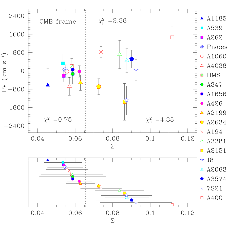
Figure 3: Cluster PV vs. $\Sigma$. Each point represents a cluster containing $\sim 10-80$ observed galaxies. The x-axis is the scatter within the cluster with respect to $\overline{\mbox{FP}}$. The abscissa is the PV as derived from redshift minus $\overline{\mbox{FP}}$ distance. The reduced $\chi^{2}$ about zero PV for the entire sample is shown at the top of the figure. $\langle\Sigma\rangle$ (vertical line) roughly marks the separation of the sample into two subgroups, over which $\chi^{2}$ rises dramatically (values shown at the bottom of the panel). The errors on $\Sigma$ are shown in the bottom panel for clarity. One can see a paucity of clusters about $\langle\Sigma\rangle$, where one would expect the density of clusters to be highest if clusters are drawn from a single population.

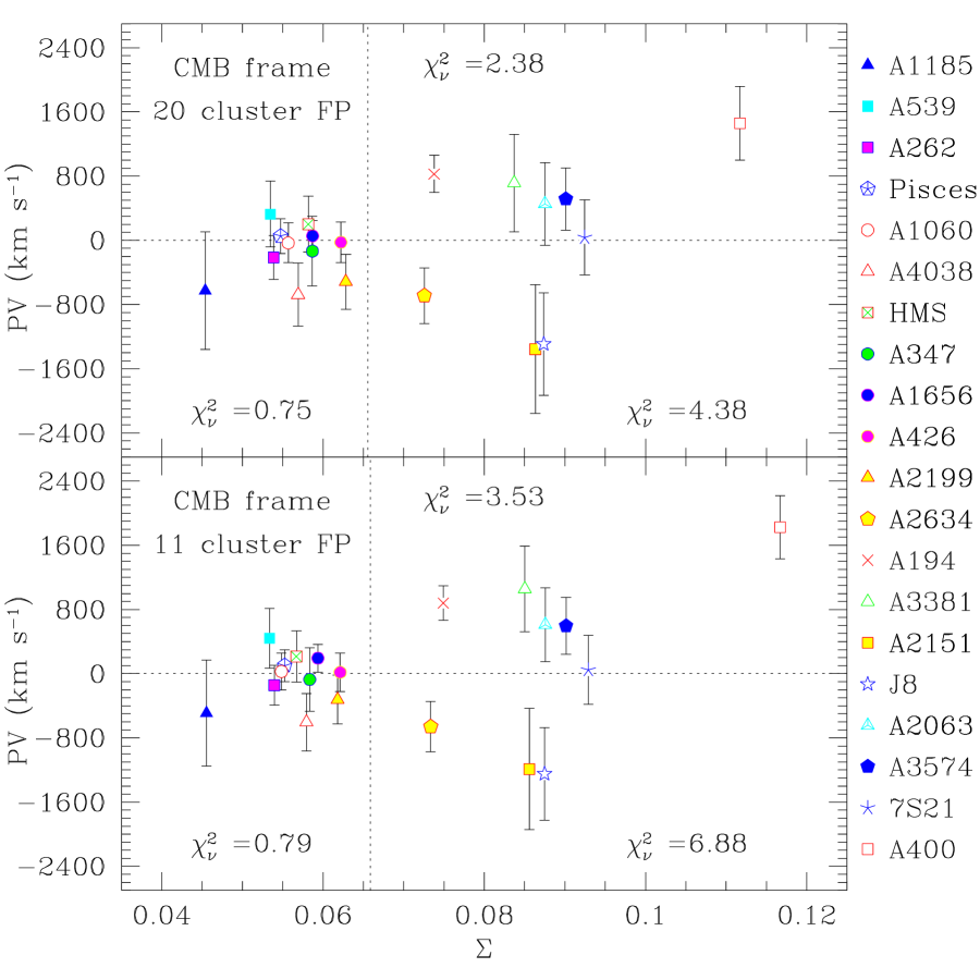
Figure 4: Comparison of the PV distribution for the 20 and 11 cluster fits. As is readily seen, use of one fit or the other does not significantly change our results.

Finally, plotting PV against $\Sigma$, we uncover an astonishing result (Figure 3). There is an obvious discontinuity in the scatter in cluster PV which occurs across the same region of $\Sigma$-space as the gap in probability already discussed. The clusters which fit $\overline{\mbox{FP}}$ well are at rest with respect to the CMB with reduced $\chi^{2}<1$ while the poor-fit clusters with ${\Sigma}>{\langle\Sigma\rangle}$ show large scatter in their PVs, $\chi^{2}=4.4$. Results from both the 20 cluster FP and 11 cluster FP are similar as can be seen in Figure 4.

While one might naively expect a correlation between $\Sigma$ and the measurement error of PV, this is not the case. If cluster ellipticals do indeed form one population, then the sample mean and sample standard deviation of a randomly drawn subset will be uncorrelated. Therefore, PV should not reflect the value of $\Sigma$. Similarly PV errors do not correlate with $\Sigma$; we therefore scale the errors by $\langle\Sigma\rangle$. As we will show in the following section, this null hypothesis is heavily disfavored as the observed non-uniformity in $\sigma_{1D}$ is highly significant.

4.3 Significant Variation in $\sigma_{1D}$

To examine the significance of the variation in $\sigma_{1D}$, we have used two approaches, linear regression and analysis of variance (ANOVA). Simple regression favors a strong correlation between PV and $\Sigma$whether we use $\langle\Sigma\rangle$ to estimate the PV errors (null hypothesis), or use the individual $\Sigma$. Straightforward weighted regressions of “$|$PV$|$ on $\Sigma$” and “$\Sigma$ on $|$PV$|$” yield slopes which are nonzero with $99.9\%$ confidence. The true slope lies somewhere between the forward and inverse regressions. But because of the two-way errors, it is difficult to decide significance analytically, so the problem can also be dealt with numerically. Resampling by complete permutation along the $\Sigma$ axis is a measure of the likelihood of the observed correlation. Permutation ignores errors in $\Sigma$ and complete mixing of the 20 points without replacement is allowed. Under the assumption of no correlation, the expected slope is zero, negative and positive slopes being equally likely. The resultant distribution shows the observed slope to be unlikely, with a probability of less than one percent.

The null hypothesis likewise fails ANOVA tests. The measured $\sigma_{1D}$ for the two subsamples of clusters (defined by the gap in $\Sigma$) are not consistent with a single PV distribution. The ratio of chi-squares disfavors the two groups being drawn from the same distribution with probability $99.94\%$. Again permuting the points along $\Sigma$$-$space allows us to estimate the probability of the present result without an assumption about the nature of the distribution. Using this bootstrapping procedure one finds the significance for the ratio of observed chi-squares is again above the $99^{th}$ percentile. The behavior of the sample both in $\Sigma$$-$space as well as in PV$-$space tends to contradict at very high levels of significance the assumption that we are observing a single population of clusters. Taken together, these statistics are convincing evidence that we are seeing two populations. If this bimodality is an intrinsic property of clusters of galaxies, then all current FP samples potentially mix together these two apparently different populations.

5 Errors in FP Distances or Peculiar Velocities?

We have established that our sample of clusters divides into two groups defined by significantly different intrinsic scatter about the FP. Additionally, we find that these two groups have radically different PV distributions. The observation that only the high-$\Sigma$ clusters show peculiar motions implies that such clusters can inject significant error into the measure of $\sigma_{1D}$. This could have the consequence of producing a spuriously large PV signal for the entire sample. Alternatively, these two groups could indeed be subject to truly different kinematics. Either scenario, suggests that the nature of the inferred PV field is sample dependent.

We find, however, no evidence that this apparent separation of the clusters into two populations is due to systematic problems with our data. There is no correlation of $\Sigma$ with cluster distance (e.g. more distant clusters do not have poorer fits). We see no effect due to data quality or data source; the clusters which we observed ourselves and the sample which was culled from the literature are equally divided between the two $\Sigma$ groups, and with the exception of A400, the quality of the imaging and spectra of all the clusters are comparable. We are also confident that our cluster samples are not significantly contaminated by field ellipticals or S0s; we are sampling the centers of clusters over an area of approximately one half square degree and our redshift criterion is $|$z$-$z${}_{mean}|\lesssim 3\sigma$, where $\sigma=$ cluster velocity dispersion. We calculate that, with the possible exception of 7S21, the expected number of field interlopers per cluster in our sample is far less than one. Addition of an Mg2 line index term to diminish cluster to cluster differences in the age/metallicity of the stellar populations also does not improve the fits. We find no strong evidence for curvature along the FP. In addition, the galaxies in each cluster cover similar ranges in log$(\sigma)$ so that we expect any error introduced by sampling different portions of the FP is at most a minor effect in our final fits and distance measurements. The high-$\Sigma$ clusters do on average have a smaller number of observed members than low-$\Sigma$ clusters. However, we would expect a small sample size to only increase the scatter of $\Sigma$ and not bias its value. Bootstrap tests on subsamples of galaxies chosen at random from Coma show this to be the case. Rather, the high-$\Sigma$ clusters are also on average the least rich clusters, and as we discuss below, there is good reason to believe that $\Sigma$ is a function of cluster richness.

If our study is relatively free from systematic errors, then our statistical analysis shows that different clusters have different amounts of intrinsic log$(\sigma)$ scatter about the FP. But what property of a cluster might be driving this observed difference? We have looked at many cluster properties as predictors of whether a cluster will be a high- or low-$\Sigma$ cluster and have found only one strong indicator : cluster X-ray luminosity, as can clearly be seen in Figure 5. The four brightest X-ray clusters, those with L${}_{\mbox{x}}>10^{44}$ erg s^-1, all have low $\Sigma$. This result suggests that early-type galaxies within the most massive, well-virialized clusters form a more homogeneous population than cluster ellipticals as a whole.

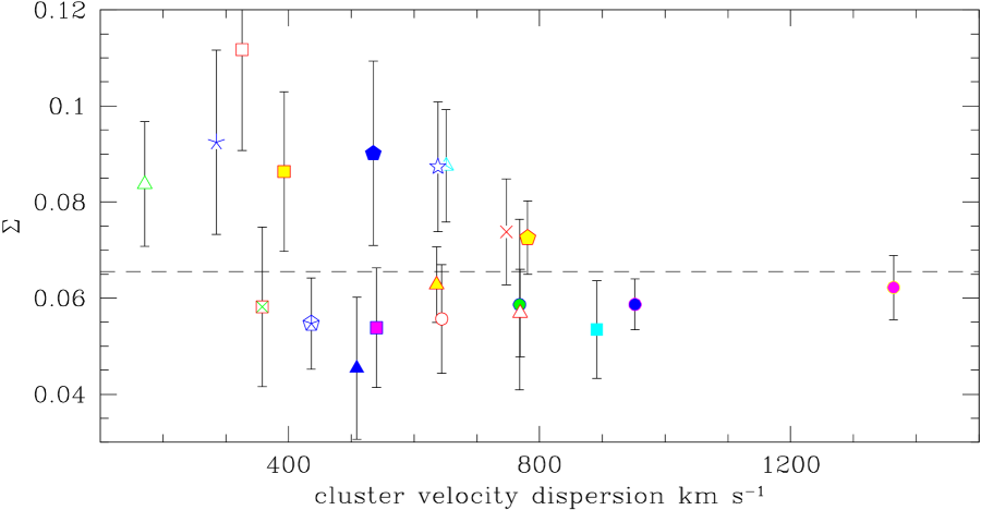
Figure 7: $\Sigma$ vs. cluster velocity dispersion. The high dispersion ($\gtrsim 800\ {\mbox{km~{}s}^{-1}}$) clusters have low $\Sigma$.

A weaker, but similar correlation, can be seen with cluster spiral fraction, which is also an indirect indicator of the dynamical evolutionary state of a cluster (see for example Dressler et al. 1997). Clusters with ${\Sigma}>0.08$ exhibit a spiral fraction of $55\pm 1\%$ compared to $42\pm 3\%$. This trend of $\Sigma$ with spiral fraction is shown in Figure 6. Similarly, $\Sigma$ appears to be related to the cluster velocity dispersion, which is itself, of course, closely tied to cluster X-ray luminosity (Figure 7). With one exception, clusters with velocity dispersions less than $400~{}{\mbox{km~{}s}^{-1}}$ tend to have high $\Sigma$ whereas those with dispersions greater than $800~{}{\mbox{km~{}s}^{-1}}$ tend to have low $\Sigma$.

There are also indications that substructure may be an important component of the increased scatter observed in some clusters. Take the case of the relatively spiral rich, low velocity dispersion clusters A2151 and A400. In A2151, the early type galaxies in the core have a mean velocity offset of $-900~{}{\mbox{km~{}s}^{-1}}$ from that of the spirals (Zabludoff et al. 1993, Dale et al. 1999b; this paper). Indeed, A2151 and A2147 are clearly entangled in a mutual interaction (e.g. Bird et al. 1995; Maccagni et al. 1995), with a component of peculiar velocity reflecting infall and/or merging of subclusters. A similar offset between mean elliptical and cluster velocity has been observed in A400 by Beers et al. (1992). In addition, both A400 and A2151 contain many examples of interacting/peculiar galaxies (see Bothun & Schommer 1982), indicating the prevalence of low velocity dispersion subgroups within the overall structure. Furthermore, substructures that are separated by $\sim 10$ Mpc or less will not be adequately resolved in kinematic distance space by the current relative indicators. An increase in $\Sigma$ can be introduced due to a range in distance along the line of site. Indeed, such a spread in distances has already been proposed for one rich, but high $\Sigma$ cluster, A2634 (see West & Bothun 1990; Scodeggio et al. 1995).

One reason for the fact that highly X-ray luminous clusters do not show significant peculiar velocity may be that X-ray luminosity coincides with the virialization of infalling structures. Whatever the source of the consistent behavior of these clusters, it appears that X-ray luminosity provides a good pre-filter for the selection of clusters to be used in PV studies. As will be shown in paper II of this series (Gibbons, Fruchter, & Bothun 2000b), such a pre-filter produces a sample that exhibits no large scale flow.

6 Conclusions

Using high-quality data and a robust fitting technique, we have determined that clusters of galaxies show a large range in quality-of-fit of their member galaxies to the FP. Statistical tests described in §4 argue that the observed separation in $\Sigma$ is significant at the $\sim 10^{-3}$ level. Additionally, an examination of the distribution of clusters along the PV axis provides further direct support for this separation. If clusters are truly random realizations of galaxies drawn from a single population, then the total sample should have, on average, a uniform $\sigma_{1D}$. Instead, when the sample is divided on the basis of the observed scatter about the FP, the two subsamples have drastically different properties in the independent dimension provided by the PV. Again, this effect is statistically strong at more than the $99\%$ level. Simply put, high-$\Sigma$ clusters have large PV and low-$\Sigma$ clusters have essentially no PV, within the observational errors. Taken together, these two results cannot be reconciled with the idea that these clusters are randomly drawn from a single population.

The behavior of $\Sigma$ appears to be an intrinsic cluster property. We have found that a subset of the clusters, the X-ray luminous clusters, exhibit a well-defined FP. This suggests that the most massive and virialized clusters possess a homogeneous population of ellipticals and therefore provide the most accurate measures of relative distance. About half of the cluster sample possess $\Sigma$ below the mean. When using this half of the sample, we find the clusters to be at rest within the CMB frame (see details in the forthcoming Gibbons et al. 2000b). The high-$\Sigma$ clusters provide the bulk of the positive PV signal when all the clusters are averaged together.

Overall, our results strongly suggest that making a cut on the r.m.s. scatter about the FP, or more strictly on cluster X-ray luminosity, will lead to a more reliable sample from which bulk flow properties can be established. The current level of disagreement between various observations of large scale flows (e.g. Table 1) may possibly reflect the fact that less reliable samples have been used.

Survey	Method	PV w.r.t. CMB (km s-1)	Survey Depth (km s-1)	$\sigma_{1D}$ (km s-1)
ACIF	BCG	$689\pm 178\;(l=343\;b=52)$	15,000	$\sim 400$
SMAC	FP	$630\pm 200\;(l=260\;b=-1)$	12,000	$\sim 350$
LP10K	IRTF	$720\pm 280\;(l=266\;b=19)$	12,000	$\sim 415$
Dale et al. 1999 a&b	IRTF	$<200$	18,000	$341\pm 93$
Watkins 1997	IRTF	–	12,000	$265^{+106}_{-75}$

Table 1: Recent Surveys : These surveys disagree in both the magnitude and the direction of their derived flows. References appear in the text. N.b. The Watkins analysis is of subsets of the Giovanelli et al. (1997) and Willick et al. (1995) surveys.

								Data	$\Sigma$			$\Sigma$
cluster	$l$(deg)		$b$(deg)		cz(km/s)	$\sigma_{clust}$	ngal	Ref.	$\overline{\mbox{FP}}$	$\alpha_{IND}$	$\beta_{IND}$	FPIND
A1656	57.	6	88.	0	7215	952	79	1,4	0.059	1.54	0.305	0.052
A400	170.	2	-44.	9	6708	326	6	1	0.112	0.86	0.301	0.149
A1185	203.	1	67.	8	9923	509	10	1	0.045	1.62	0.267	0.057
A2063	12.	9	49.	7	10406	651	17	1	0.088	1.88	0.299	0.096
A2151	31.	6	44.	5	10188	393	9	1	0.086	1.50	0.257	0.070
HMS0122	130.	2	-27.	0	4636	358	9	5	0.058	1.87	0.293	0.068
J8	150.	3	-34.	4	9425	638	13	5	0.087	1.37	0.340	0.096
Pisces	126.	8	-30.	3	4714	436	25	5	0.055	1.10	0.369	0.047
A2199	62.	9	43.	7	8947	636	36	4	0.063	1.32	0.359	0.059
A262	136.	6	-25.	1	4417	540	15	1,5	0.054	1.67	0.308	0.061
A2634	103.	5	-33.	7	9132	781	38	1,4	0.073	1.37	0.311	0.072
A347	140.	7	-18.	1	5312	768	8	5	0.059	1.26	0.348	0.061
A426	150.	5	-13.	7	5139	1364	49	1,5	0.062	1.45	0.357	0.065
7S21	113.	8	-40.	0	5517	285	7	5	0.092	1.94	0.179	0.130
A194	142.	2	-62.	9	5122	747	19	3,2	0.074	1.04	0.333	0.069
A539	195.	6	-17.	6	8615	891	22	3	0.053	1.46	0.327	0.055
A3381	240.	3	-22.	7	11471	171	14	3	0.084	1.72	0.227	0.076
A3574	317.	4	31.	0	4873	535	7	3	0.090	1.49	0.352	0.115
A4038	25.	3	-75.	8	8473	769	27	3,2	0.057	1.36	0.342	0.061
A1060	269.	6	26.	5	3976	644	18	3,2	0.056	1.58	0.347	0.056
1 = this work; 2 = Lucey & Carter 1988 (LC88);
3 = Jørgensen, Franx & Kjærgaard 1995a,1995b (JFK95a,JFK95b);
4 = Lucey, Guzmán, Smith & Carter 1997 (LGSC97);
5 = Smith, Lucey, Hudson & Steel 1997 (SLHS97)

Table 2: The Cluster Sample : column (1) cluster name; (2-3) cluster position in Galactic coordinates; (4) heliocentric redshift; (5) cluster velocity dispersion; (6) number of observed galaxies; (7) data references as defined above; (7) scatter about the average FP; (8-9) FP parameters for the fits to individual clusters.

Figure 1: (a) The $\overline{\mbox{FP}}$ for the entire sample of 428 galaxies. This projection shows the scatter about log($r_{e}$). (b) The significance of $\chi^{2}$ about $\overline{\mbox{FP}}$ for each cluster vs. FP scatter. The gap seen in probability space is highly significant, making it unlikely that all clusters have been drawn from a single population.

Figure 2: (a) The $\overline{\mbox{FP}}$ for the 11 best-fit clusters. (b) Same as Figure 1b but for the 11 cluster FP fit. When fit this way the high-$\Sigma$ clusters are outliers, falling in the upper $5\%$ tail in probability space, while the rest are consistent with being uniformly distributed.

Figure 5: $\Sigma$ vs. X-ray luminosity, L${}_{\mbox{x}}$. Note that the massive, virialized clusters fit the FP well, while the quality-of-fit for the lower mass clusters cannot be predicted. The most X-ray bright clusters (L${}_{\mbox{x}}\gtrsim 10^{44}$ erg s^-1) are labeled. The clusters for which there exist no X-ray data are shown along the left side of the panel. L${}_{\mbox{x}}$ from White, Jones, & Forman (1997).

Figure 6: $\Sigma$ vs. cluster spiral fraction (SF). A weak correlation between these two variables is evident and is in the same sense as expected from the X-ray data. Spiral fractions from Dressler 1980.

References

- (1) Aaronson, M., Bothun, G. D., Mould, J. R., Huchra, J. P., Schommer, R. A., & Cornell, M. E. 1986, ApJ, 302, 536
- (2) Akritas, M. G. & Bershady, M. A. 1996, ApJ, 470, 706
- (3) Bahcall, N. A. & Fan, X. 1998, ApJ, 504, 1
- (4) Bird, C. M., Davis, D. S., & Beers, T. C. 1995, AJ, 109, 920
- (5) Bothun, G. D. & Schommer, R. A. 1982, AJ, 87, 1368
- (6) Borgani, S., da Costa, L. N., Freudling, W., Giovanelli, R., Haynes, M. P., Salzer, J., & Wegner, G. 1997, ApJL, 482, 121
- (7) Burstein, D. & Heiles, C. 1984, ApJS, 54, 33
- (8) Beers, T. C., Gebhardt, K., Huchra, J. P., Forman, W., Jones, C., & Bothun, G. D. 1992, ApJ, 400, 410
- (9) Coleman, G. D., Wu, C-C, & Weedman, D. W. 1980, ApJS, 43, 393
- (10) Courteau, S., Faber, S. M., Dressler, A., & Willick, J. A. 1993, ApJL, 412, 51
- (11) Carvalho, de R. R. & Djorgovski, S. 1989, ApJ Lett., 341, 37
- (12) Carvalho, de R. R. & Djorgovski, S. 1992, ApJ Lett., 389, 49
- (13) Dale, D. A., Giovanelli, R., Haynes, M. P., Campusano, L. E., Hardy, E., & Borgani, S. 1999a, ApJL, 510, 11
- (14) Dale, D. A., Giovanelli, R., Haynes, M. P., Campusano, L. E., & Hardy, E. 1999b, AJ, 118, 1489
- (15) Djorgovski, S. & Davis, M. 1987, ApJ, 313, 59
- (16) Dressler, A. 1987, ApJ, 317, 1
- (17) Dressler, A., Oemler Jr., A., Couch, W. J., Smail, I., Ellis, R. S., Barger, A., Butcher, H., Poggianti, B. M., & Sharples, R. M. 1997, ApJ, 490, 577
- (18) Dressler, A., Lynden-Bell, D., Burstein, D., Davies, R. L., Faber, S. M., Wegner, G., & Terlevich, R. 1987, ApJ, 313, 42
- (19) Franx, M., Illingworth, G., & Heckman, T. 1989, ApJ, 344, 613
- (20) Gibbons, R. A., Fruchter, A. S., & Bothun, G. D. 2000b, in prep
- (21) Gibbons, R. A., Fruchter, A. S., & Bothun, G. D. 2000c, in prep
- (22) Giovanelli, R., Haynes, M. P., Herter, R., Vogt, N. P., Wegner, G., Salzer, J. J., da Costa, L. N., & Freundling, W. 1997, AJ, 113, 22
- (23) Giovanelli, R., Haynes, M. P., Wegner, G., da Costa, L. N., Freundling, W., & Salzer, J. J. 1996, ApJ Lett., 464, 99
- (24) Gregg, M. D. 1995, ApJ, 443, 527
- (25) Guzmán, R. & Lucey, J. R. 1993, MNRAS, 263, 47
- (26) Hudson, M. J., Lucey, J. R., Smith, R. J., & Steel J. 1997, MNRAS, 291, 461
- (27) Hudson, M. J., Smith, R. J., Lucey, J. R., Schlegel, D. J., & Davies, R. L. 1999, ApJL, 512, 79
- (28) Jacoby, G. H., Branch, D., Ciardullo, R., Davies, R. L., Harris, W. E., Pierce, M. J., Pritchet, C. J., Tonry, J. L., & Welch, D. L. 1992, PASP, 104, 599
- (29) Jørgensen, I., Franx, M., & Kjærgaard, P. 1995a, MNRAS, 273, 1097
- (30) Jørgensen, I., Franx, M., & Kjærgaard, P. 1995b, MNRAS, 276, 1341
- (31) Jørgensen, I., Franx, M., & Kjærgaard, P. 1996, MNRAS, 280, 167
- (32) Kogut, A. et al. 1993, ApJ, 419, 1
- (33) Kelson, D. D., Illingworth, G. D., van Dokkum, P. G., & Franx, M. 1999, astro-ph/9911065 (accepted for publication in the ApJ)
- (34) Kirkpatrick, S., Gelatt, C. D., Vecchi, M. P. 1983, Science, 220, 671
- (35) Kriss, J. 1992, IRAF package stsdas.contrib.redshift
- (36) Lauer, T. & Postman, M. 1994, ApJ, 425, 418
- (37) Lucey, J. R., Bower, R. G., & Ellis, R. S. 1991, MNRAS, 249, 755
- (38) Lucey, J. R. & Carter, D. 1988, MNRAS, 235, 1177
- (39) Lucey, J. R., Guzmán, R., Smith, R. J., & Carter, D. 1997, MNRAS, 287, 899
- (40) Lynden-Bell, D., Faber, S. M., Burstein, D., Davies, R. L., Dressler, A., Terlevich, R. J., & Wegner, G. 1988, ApJ, 326, 19
- (41) Maccagni, D., Garilli, B., & Tarenghi, M. 1995, AJ, 109, 465
- (42) Metropolis, N., Rosenbluth, A., Rosenbluth, M., Teller, A., & Teller, E. 1953, J. Chem. Phys., 21, 1087
- (43) Sargent, W. L. W., Schechter, P. L., Boksenberg, A., & Shortridge, K. 1977, ApJ, 212, 326
- (44) Scodeggio, M., Giovanelli, R., & Haynes, M. P. 1998, AJ, 116, 2728
- (45) Scodeggio, M., Solanes, J. M., Giovanelli, R., & Haynes, M. 1995, ApJ, 444,41
- (46) Smith, R. J., Lucey, J. R., Hudson, M. J., & Steel J. 1997, MNRAS, 291, 461
- (47) Strauss, M. A., Cen, R., Ostriker, J. P., Lauer, T. R., & Postman, M. 1995, ApJ, 444, 507
- (48) Tonry, J. L., & Davis, M. 1979, AJ, 84, 1511
- (49) Vanderbilt, D. & Louie, S. G. 1984, J. Comp. Phys., 56, 259
- (50) Watkins, R. 1997, MNRAS, 292, 59
- (51) West, M. J. & Bothun, G. D. 1990, ApJ, 350, 36
- (52) Whitmore, B. C., Gilmore, D. M., & Jones, C. 1993, ApJ, 407, 489
- (53) White, D. A., Jones, C., & Forman, W. 1997, MNRAS, 292, 419
- (54) Willick, J. A., Courteau S., Faber, S. M., Burstein, D., & Dekel, A. 1995, ApJ, 446, 12
- (55) Zabludoff, A. I., Geller, M. J., Huchra, J. P., & Vogeley, M. S. 1993, AJ, 106, 1273