Galaxy Cluster Shapes and Systematic Errors in H₀
Measured by the Sunyaev-Zel’dovich Effect

Abstract

Imaging of the Sunyaev-Zel’dovich (SZ) effect in galaxy clusters combined with cluster plasma x-ray diagnostics can measure the cosmic distance scale to high redshift. However, projecting the inverse-Compton scattering and x-ray emission along the cluster line-of-sight introduces systematic errors in the Hubble constant, $H_{0}$, because the true shape of the cluster is not known. In this paper I present a study of the systematic errors in the value of $H_{0}$, as determined by the x-ray and SZ properties of theoretical samples of triaxial isothermal “beta” model clusters, caused by projection effects and observer orientation relative to the model clusters’ principal axes. I calculate three estimates for $H_{0}$ for each cluster, based on their large and small apparent angular core radii, and their arithmetic mean. I demonstrate that the estimates for $H_{0}$ for a sample of 25 clusters have limited systematic error: the 99.7% confidence intervals for the mean estimated $H_{0}$ analyzing the clusters using either their large or mean angular core radius are within $\simeq 14\%$ of the “true” (assumed) value of $H_{0}$ (and enclose it), for a triaxial beta model cluster sample possessing a distribution of apparent x-ray cluster ellipticities consistent with that of observed x-ray clusters. This limit on the systematic error in $H_{0}$ caused by cluster shape assumes that each sample beta model cluster has fixed shape; deviations from constant shape within the clusters may introduce additional uncertainty or bias into this result.

1. Introduction

There has been a substantial effort to detect the Sunyaev-Zel’dovich (SZ) effect from galaxy clusters (Sunyaev & Zel’dovich 1972) and to analyze its distortion of the cosmic microwave background radiation (CMB) in conjunction with cluster x-ray properties to derive the cluster cosmological angular-diameter distance and thus estimates of the cosmological parameters $H_{0}$ and $q_{0}$ (Gunn 1978, Silk & White 1978, Cavaliere, Danese, & DeZotti 1979, Birkinshaw 1979; see also Birkinshaw 1998, and references therein). This method provides a distance determination for the cluster that is independent of the “cosmic distance ladder” of Cepheid variables or supernovæ, and is potentially effective for clusters at high redshift ($z\simeq 1$). Centimeter-wavelength interferometry optimized for imaging the SZ effect from galaxy clusters has been recently developed (Carlstrom, Joy, and Grego 1996; Grainge et al. 1996;). This allows high-resolution x-ray and radio images of clusters to be analyzed simultaneously. The results of fits of both the x-ray and radio images to simple cluster-plasma models will yield improved estimates of $H_{0}$, and systematic errors in the measured value of $H_{0}$ are likely to be a significant limit to its accuracy.

Sources of systematic errors in the SZ-determined $H_{0}$ and $q_{0}$ can originate from the assumptions made in modeling the cluster plasma: ignorance of the cluster plasma’s true three-dimensional distribution and inadequate treatment of the physical state of the cluster plasma. Radio and x-ray images only provide the projected x-ray surface brightness and CMB decrement. For the analysis to proceed some assumption must be made about the cluster size along the line of sight; e.g. , one assumes that cluster has spherical or ellipsoidal symmetry. The modeling of physical state of cluster plasma for SZ analysis has generally assumed that the plasma was of a single phase and temperature, using the somewhat ad hoc “beta” model for electron density, $n_{e}({\rm{\bf{r}}})\propto(1+r^{2}/r_{c}^{2})^{-3\beta/2}$, where $r_{c}$ is cluster’s “core radius”, within which the density is relatively flat. The beta model can be argued as a possible distribution for the plasma in a dynamically relaxed isothermal cluster in hydrostatic equilibrium (e.g. , Cavaliere & Frusco-Femiano 1978; Sarazin 1986), but its usefulness is more empirical; many x-ray images of clusters fit a beta model reasonably well (Mohr et al. 1999; see §4). Also, studies of the distribution of SZ systematic errors caused by cluster shape and orientation (and other effects) based on the results of a large ensemble of numerically simulated clusters have yet to be completed; current results are for a small set of simulated clusters (see §4). Thus, three-dimensional “toy model” estimates for the effects of cluster shape are a useful first step in estimating these errors, and can help identify the physical sources of bias and scatter in $H_{0}$ estimates from simulated clusters.

In this paper I study the systematic errors in the value of $H_{0}$, measured by SZ and x-ray observations, caused by effects of cluster shape. This study consists of two parts. First, I create theoretical galaxy cluster samples, where each cluster’s plasma distribution follows a triaxial isothermal beta-model (§2), possessing three independent core radii. I use the triaxial beta model because it is a simple three-dimensional generalization of the spherical or ellipsoidal beta models (commonly used in SZ analysis) that demonstrates the effects of shape and orientation on the uncertainties in $H_{0}$ determined by SZ observations. The triaxial beta model also produces simple analytical functions for the CMB decrement and x-ray surface brightness so results for large samples of clusters can be easily calculated.

I create numerical distributions clusters by uniformly and independently sampling the plasma core radii, constraining them by a minimum ratio between any two core radii of a sample cluster. These samples are uniform in the plane of allowed cluster oblateness and ellipticity. The clusters are placed in the sky with a random orientation to our line of sight. I identify a cluster sample with an optimum asphericity that has a distribution of apparent cluster ellipticities that is consistent with that of observed x-ray clusters (Mohr et al. 1995; see §3).

Second, I analyze the clusters of the theoretical sample to determine their distance as if they were either spherical or an ellipsoid of rotation, as in done in observational analysis (e.g. Hughes & Birkinshaw 1998). An important unknown quantity is an ellipsoidal cluster’s inclination angle $i$; the estimated value for $H_{0}$ will vary greatly with $i$. However, since our theoretical clusters are actually three-dimensional, specifying a single inclination angle is artifical. Therefore, I analyze each cluster very simply as if its inclination angle $i=90^{\circ}$, i.e. , that the core radii for the clusters are not altered by projection effects, and then study the distribution of the estimates for $H_{0}$ for a large number of sample clusters. The apparent shape of a sample cluster’s x-ray surface brightness will be elliptical, with a large and small angular core radius, $\theta^{+}\geq\theta^{-}$. I calculate two different estimates of $H_{0}$ which are proportional to either $\theta^{+}$ or $\theta^{-}$, designated $\hat{H}_{0}^{+}$ and $\hat{H}_{0}^{-}$. I also calculate an estimate $\hat{H}_{0}^{\rm avg}$, by using the arithmetic average of $\theta^{+}$ and $\theta^{-}$.

I find that the sample means of the estimates $\hat{H}_{0}^{+}$ and $\hat{H}_{0}^{\rm avg}$ fall within $\simeq 5\%$ of $H_{0}$ for the optimal sample. The sample distribution of $\hat{H}_{0}^{-}$ shows greatest bias, with a mean for $\hat{H}_{0}^{-}$ that underestimates $H_{0}$ by $\simeq 14\%$ for my optimal cluster sample.

As a predictor for SZ observations, I also calculate estimates for $H_{0}$ averaged for 1000 realizations of a sample of 25 clusters. I find that the systematic errors caused by cluster shape are limited: the $99.7\%$ confidence intervals for $\hat{H}_{0}^{+}$ and $\hat{H}_{0}^{\rm avg}$ include the assumed value of $H_{0}$ for my optimal cluster sample, and do not extend beyond $\simeq 14\%$ from $H_{0}$. The $99.7\%$ confidence interval for $\hat{H}_{0}^{-}$ does not include $H_{0}$, indicating that it may not be a useful parameter for distance estimation.

The structure of this paper is as follows. In section §2 I describe the triaxial beta model for the cluster plasma, and describe the analytic expressions for their CMB decrement and x-ray surface brightness. I also describe the construction of samples of theoretical clusters, distinguished by their degree of triaxiality, and describe the manner in which I analyze the apparent clusters to determine values for $H_{0}$. I present our results in §3, followed by a summary and discussion – noting some of the limitations of this beta model based analysis – in §4.

2. Method

2.1. Triaxial beta model clusters

The distribution of cluster plasma is described by an isothermal “beta” model. The electron density at a position within the cluster ${\rm{\bf{r}}}=x_{1}{\hat{\rm{\bf{x}}}}_{1}+x_{2}{\hat{\rm{\bf{x}}}}_{2}+x_{3}{\hat{\rm{\bf{x}}}}_{3}$, measured in the observer’s coordinates, is given by

$$n_{e}({\rm{\bf{r}}})=n_{e0}\bigl{(}1+{\rm{\bf{r}}}\cdot{\rm{\bf{M}}}\cdot{\rm{\bf{r}}})^{-{3\over 2}\beta},$$ (1)

where the matrix ${\rm{\bf{M}}}$ describes a cluster’s shape and orientation of its principal axes to the observer, and $\beta$ is an exponent with the nominal range $\text@frac{1}{2}<\beta\leq 1$. The maps of x-ray surface brightness $S_{X}$ and cosmic-microwave background decrement $\delta T_{r}$ in sky angular coordinates $(\vartheta,\varphi)$ (measured from the cluster center ${\rm{\bf{r}}}=0$) are given by integrals of the x-ray emissivity and electron pressure over the line-of-sight (defined here as $x_{1}$) though the cluster;

$$S_{X}(\vartheta,\varphi)={{1}\over{4\pi(1+z)^{3}}}\,\int\,\Lambda_{X}(T_{e}({\rm{\bf{r}}}))\,n_{e}^{2}({\rm{\bf{r}}})\>dl$$ (2)

and

$$\delta T_{r}(\vartheta,\varphi)\equiv{{\Delta T_{r}}\over{T_{r}}}(\vartheta,\varphi)=-2\,{{k_{B}\sigma_{T}}\over{m_{e}c^{2}}}\,\int\,T_{e}({\rm{\bf{r}}})\,n_{e}({\rm{\bf{r}}})\>dl.$$ (3)

Here $T_{e}$ is the electron temperature, hereafter assumed to be constant, $\Lambda_{X}(T_{e})$ is the plasma emission function over a prescribed x-ray bandwidth at temperature $T_{e}$, and $z$ is the cluster redshift.

For a triaxial isothermal beta model plasma described by equation (1), then integrating equation (2) by choosing $dl=dx_{1}$ gives $S_{X}$ to be

$$S_{X}(\vartheta,\varphi)={{B({{1}\over{2}},3\beta-{{1}\over{2}})}\over{4\pi}}\;{{n_{0e}^{2}\Lambda_{X}(T_{e})}\over{(1+z)^{3}}}\;{{L_{eff}}\over{\chi(\vartheta,\varphi)^{3\beta-{{1}\over{2}}}}},$$ (4)

where $\chi(\vartheta,\varphi)$ is a quadratic function of the sky angular coordinates $\vartheta$ and $\varphi$, describing elliptical isophotes. Along the line of sight of the center $\chi(0,0)=1$. The quantity $B(q,r)$ is the beta function. The quantity $L_{eff}$ is an effective column length for the plasma along the line of sight through the cluster:

$$L_{eff}^{{}^{\rm triaxial}} = {{1}\over{\sqrt{M_{11}}}}$$ (5)

$$= \biggl{\{}{{\cos^{2}\alpha_{1}}\over{r_{c1}^{2}}}+\sin^{2}\alpha_{2}\bigl{(}{{\cos^{2}\alpha_{3}}\over{r_{c2}^{2}}}+{{\sin^{2}\alpha_{3}}\over{r_{c3}^{2}}}\bigr{)}\biggr{\}}^{-1/2}.$$

The quantities $(r_{c1},r_{c2},r_{c3})$ are the cluster core radii, and $(\alpha_{1},\alpha_{2},\alpha_{3})$ are the rotation angles of the cluster principal axes relative to the observer. The coefficients in the quadratic function $\chi(\vartheta,\varphi)$ are also functions of the cluster core radii and its orientation.

By integrating equation (3) in exactly the same manner, $\delta T_{r}$ can be shown to be

$$\delta T_{r}(\vartheta,\varphi)=-B({{1}\over{2}},{{3}\over{2}}\beta-{{1}\over{2}})\;n_{e0}\sigma_{T}\,{{k_{B}T_{e}}\over{m_{e}c^{2}}}\;{{L_{eff}}\over{\chi(\vartheta,\varphi)^{{{3}\over{2}}\beta-{{1}\over{2}}}}}.$$ (6)

The value of $L_{eff}$ determined from observations by relating $S_{X}$ and $\delta T_{r}$ observed for the cluster. For example, $L_{eff}$ can be determined by the values of $\delta T_{r}$ and $S_{X}$ measured at the cluster’s center:

$$L_{eff}={{B({{1}\over{2}},3\beta-{{1}\over{2}})}\over{B^{2}({{1}\over{2}},{{3}\over{2}}\beta-{{1}\over{2}})}}{{1}\over{(1+z)^{3}}}{{\Lambda_{X}(T_{e})}\over{4\pi\sigma_{T}^{2}}}\biggl{(}{{m_{e}c^{2}}\over{k_{B}T_{e}}}\biggr{)}^{2}{{\delta T_{r}^{2}(0,0)}\over{S_{X}(0,0)}}.$$ (7)

The cluster’s cosmological angular diameter distance $D_{\theta}(z;H_{0},q_{0})$ is then inferred by equating the measured $L_{eff}$ to that derived from a model for the cluster. Recent efforts to fit the cluster $S_{X}$ (Hughes and Birkinshaw 1998) assume that the cluster is either an oblate or prolate ellipsoid in shape as well as isothermal; this assumption about shape is reasonable when no information can be known about the structure of the cluster along the line of sight. However, the dependence of $L_{eff}$ on the cluster’s apparent major and minor axes for an ellipsoidal beta model is different than that for a triaxial cluster.

$$L_{eff}^{{}^{\rm ellipsoidal}}=D_{\theta}(z;H_{0},q_{0})\biggl{\{}{{\cos^{2}i}\over{\theta_{c2}^{2}}}+{{\sin^{2}i}\over{\theta_{c1}^{2}}}\biggr{\}}^{-1/2},$$ (8)

where $\theta_{c1}$ and $\theta_{c2}$ are an ellipsoidal clusters’ angular axes; $\theta_{c1}>\theta_{c2}$ describes an oblate ellipsoid and $\theta_{c1}<\theta_{c2}$ describes a prolate ellipsoid. The quantity $i$ is the inclination angle of the symmetry axis.

If the cluster is triaxial, the observed $L_{eff}$ will be equal to that of equation (5). However, analyzing the cluster as an apparent ellipsoid with equation (8) will produce a systematic error in the inferred value of $D_{\theta}$, and thus in cosmological parameters $H_{0}$ and $q_{0}$.

2.2. The theoretical cluster samples

I generate triaxial beta-model clusters choosing a set of core radii $(r_{c1},r_{c2},r_{c3})$ from a random uniform distribution for the ratio of two of the core radii, $r_{c2}$ and $r_{c3}$, with respect to $r_{c1}$. Both $r_{c2}$ and $r_{c3}$ are assumed to be a random fraction of the length of $r_{c1}$, but bounded below by a minimum value. This minimum value is not known a priori but can be chosen to optimize the observed ellipticity of x-ray clusters (see below). Clusters are only distinguished by their core radii; I do not create a distribution for the clusters’ $\beta$-values nor any other quantity except core radii. Spherical beta model fits to real clusters appear to exhibit correlation between core radius and the value of $\beta$ (Neumann and Arnaud 1999). However, the observed correlation for beta model clusters is not convolved by cluster shape projection. This is shown in the expressions for the x-ray surface brightness $S_{X}$, equation (4), and SZ CMB decrement, $\delta T_{r}$, equation (6). The profile exponents for both of these quantities are not functions of the individual core radii nor of rotation angles; nor are the major and minor axes of the observed elliptical cluster ($\theta^{+}$ and $\theta^{-}$, see §2.3) functions of $\beta$; they are only functions of the sample cluster’s core radii and the rotation angles. Also, I am not considering a distribution of the magnitude of the cluster core radii, but the distribution of the cluster triaxiality (see §2.3).

I rule out bias in the cluster samples toward a net oblateness or prolateness by checking for uniform sampling in the ellipticity-prolateness $(E,P)$ plane, given by Thomas et al. (1998) as

$$E\equiv{{1}\over{2}}{{r_{c2}^{2}(r_{c1}^{2}-r_{c3}^{2})}\over{r_{c2}^{2}r_{c3}^{2}+r_{c1}^{2}r_{c3}^{2}+r_{c1}^{2}r_{c2}^{2}}},$$ (9)

and

$$P\equiv{{1}\over{2}}{{r_{c2}^{2}r_{c3}^{2}-2r_{c1}^{2}r_{c3}^{2}+r_{c1}^{2}r_{c2}^{2}}\over{r_{c2}^{2}r_{c3}^{2}+r_{c1}^{2}r_{c3}^{2}+r_{c1}^{2}r_{c2}^{2}}}.$$ (10)

Strictly prolate and oblate clusters fall onto the lines $P=-E$ and $P=E$ respectively, with length determined by the lower bound of the ratio between core radii. My optimal sample, described below, uniformly covers the allowed region in the $(E,P)$ plane, which is a triangle proscribed by the prolate and oblate lines and the line connecting their endpoints.

How well does the triaxial beta model reproduce the observed shapes of x-ray clusters that could be used for SZ analysis? A study of 65 Einstein x-ray clusters by Mohr et al. (1995) found an emission-weighted mean ellipticity of $0.20\,\pm 0.12$, while McMillan, Kowalski, and Ulmer (1989) found a mean ellipticity of $0.24\,\pm 0.14$ for 49 Einstein Abell clusters. In both of these studies clusters were included with substantial flattening caused by recent merging, or with cooling inflows which can make the cluster appear more spherical. A more appropriate sample for comparison would be one which excludes these effects. If I eliminate clusters that are apparent mergers from the Mohr et al. sample (8 out of 12 clusters with ellipticities of $0.3$ or greater with apparent subclustering) and clusters in which cooling inflows may exist (as measured by central cooling times of 10 Gyr or less; an additional 17 clusters), then the mean ellipticity of the remaining subset is $0.18\,\pm 0.09$. I find that a triaxial beta model cluster sample where the minimum ratio between any two core radii to be $\simeq 0.65$ produces a distribution of apparent ellipticities that is consistent with this subset of the Mohr et al. sample (figure 1). A Kolmogorov-Smirnov test between these samples indicates the ellipticity distributions are statistically indistinguishable, with a maximum difference between the two cumulative distributions of $d=0.12$, and a probability that the two samples are drawn from the same distribution of $\simeq 69\%$.

2.3. The analysis

The systematic error in analyzing the clusters arises from assuming that an apparent cluster is either a prolate or an oblate ellipsoid, when it is in fact triaxial. The apparent elliptical image of the cluster will have a major and minor axis, $\theta^{+}$ and $\theta^{-}$; these are the “angular core radii” for the x-ray and SZ images. Using equation (5) and the function $\chi(\vartheta,\varphi)$, $\theta^{+}$, $\theta^{-}$, and $L_{eff}$ are determined for a given triaxial cluster. The observational analysis proceeds as if the observed $\theta^{+}$ and $\theta^{-}$ are that of an ellipsoidal cluster, inclined to the line of sight by an unknown angle $i$. The apparent cluster distance $\hat{D}_{\theta}$ for an ellipsoidal cluster is related to $\theta^{+}$, $\theta^{-}$, $L_{eff}$, and $i$ by deprojecting the cluster axes and using equation (8):

$$L_{eff}=\hat{D}_{\theta}(z;\hat{H}_{0},\hat{q}_{0})\cases{\sqrt{{{\theta^{-^{2}}(\theta^{+^{2}}-\theta^{-^{2}}\cos^{2}i)}\over{\theta^{+^{2}}\sin^{2}i}}},&{\rm(prolate)};\cr\sqrt{{{\theta^{+^{2}}(\theta^{-^{2}}-\theta^{+^{2}}\cos^{2}i)}\over{\theta^{-^{2}}\sin^{2}i}}},&{\rm(oblate).}\cr}$$ (11)

Equating $L_{eff}$ of equation (11) with that for the triaxial cluster, then in general $\hat{D}_{\theta}$ will not be equal to the actual distance $D_{\theta}$. This leads to erroneous values for the apparent cosmological parameters $H_{0}$ and $q_{0}$.

Since the sample clusters are intrinsically triaxial, using estimators (11) for $H_{0}$ based on an ellipsoidal cluster model with a single inclination angle $i$ is artificial; there is no single angle that characterizes the orientation of a cluster to the line of sight, unless a sample cluster’s core radii had been accidentally chosen to be roughly prolate or oblate. Therefore, I collapse the dependency on $i$ and assume $i\equiv 90^{\circ}$, and use only a cluster’s observed $\theta^{+}$ and $\theta^{-}$. I compose three estimates for $H_{0}$ for each cluster: $\hat{H}_{0}^{+}\propto\theta^{+}$, $\hat{H}_{0}^{-}\propto\theta^{-}$, and $\hat{H}_{0}^{\rm avg}\propto\text@frac{1}{2}(\theta^{+}+\theta^{-})$. These estimates are ordered $\hat{H}_{0}^{+}\geq\hat{H}_{0}^{\rm avg}\geq\hat{H}_{0}^{-}$. The estimate $\hat{H}_{0}^{+}$ is equivalent to assuming the observed cluster an oblate ellipsoid, while the estimate $\hat{H}_{0}^{-}$ is for the cluster as a prolate ellipsoid, both viewed as if the axis of rotation were in the plane of the sky. I study the distribution of these estimators for $H_{0}$ for a sample of triaxial clusters drawn from the distribution described in §$2.2$. The cosmological parameter $q_{0}$ is fixed to be zero, so that $\hat{D}_{\theta}=c\hat{H}_{0}^{-1}z(1+\text@frac{1}{2}z)/(1+z)^{2}$. As mentioned in §2.2, I am sampling clusters only by a distribtution in their triaxiality, and I do not use the magnitude of the core radii. Thus the estimators $\hat{H}_{0}$ are determined with respect to an assumed value of $H_{0}$.

3. Results

Figure 1 shows the distributions of the values of $\hat{H}_{0}^{+}$ and $\hat{H}_{0}^{-}$ inferred from the cluster apparent angular axes, a scatterplot of these estimates (one point per cluster), and the distribution of apparent cluster ellipticities, for our optimal theoretical beta model sample (with a minimum ratio of core radii of $0.65$). Figure 2 shows the distribution of of $\hat{H}_{0}^{\rm avg}$ for this cluster sample.

The distributions of $\hat{H}_{0}^{+}$ has sample mean that is within $\simeq 8\%$ of the assumed value of $H_{0}$. The distribution of $\hat{H}_{0}^{-}$ is more biased (i.e. , lower) in sample mean value, which is expected since for every sample cluster the value of $\hat{H}_{0}^{-}$ is constrained to be lower in value than $\hat{H}_{0}^{+}$.

I also studied the distribution of the $H_{0}$ estimates for clusters samples with greater asphericity. For a cluster sample with a minimum ratio of core radii of $0.5$, the estimate distributions broaden significantly, and the sample deviations nearly double. The distribution of $\hat{H}_{0}^{\rm avg}$ also exhibit broadening with greater asphericity, but still has a mean value within $\simeq 5\%$ of $H_{0}$. All of the means are relatively insensitive to the samples’ degree of asphericity.

What then is the expected systematic error in the measured $H_{0}$ caused by cluster shape for a practical-sized sample of clusters? The $99.7\%$ confidence intervals for the mean values $\hat{H}_{0}^{+}$, $\hat{H}_{0}^{-}$, and $\hat{H}_{0}^{\rm avg}$, based on 1000 realizations of a 25-cluster sample are summarized in Table 1. The confidence intervals for $\hat{H}_{0}^{+}$ and $\hat{H}_{0}^{\rm avg}$ include the assumed value of $H_{0}$ for the optimal cluster sample, and even for samples with even greater asphericity. For the optimal cluster sample the confidence intervals for $\hat{H}_{0}^{+}$ and $\hat{H}_{0}^{\rm avg}$ do not extend beyond $\simeq 14\%$ from $H_{0}$. The $99.7\%$ confidence interval for $\hat{H}_{0}^{-}$ does not include the assumed value of $H_{0}$.

Minimum ratio of core radii	$\hat{H}_{0}^{+}/H_{0}$	$\hat{H}_{0}^{-}/H_{0}$	$\hat{H}_{0}^{\rm avg}/H_{0}$
0.65	0.94 - 1.14	0.78 - 0.97	0.87 - 1.05

Table 1$99.7\%$ confidence intervals for 25-cluster sample mean of $\hat{H}_{0}$. The mininum ratio between core radii is $0.65$

4. Summary and Discussion

The high-resolution imaging of the SZ effect in galaxy clusters in combination with cluster plasma x-ray diagnostics is a powerful technique for measuring the cosmic distance scale. This method is sensitive to the projection of the cluster’s inverse-Compton scattering and x-ray emission, which depend on plasma density and temperature along the cluster line-of-sight.

In this paper I have estimated the systematic errors in the SZ-determined Hubble constant caused only by the projection effects of cluster shape. I use a triaxial beta model to represent the clusters’ gas because it is the simplest generalization of the ubiquitous spherical and ellipsoidal beta models that can demonstrate the effects of cluster shape and orientation on measurements of $H_{0}$. The triaxial beta model has analytic expressions for the clusters’ CMB decrement and x-ray surface brightness, so that the statistics for measured $H_{0}$ for a very large number of clusters are easily computed.

Ideal clusters for SZ analysis would possess no obvious substructure nor evidence of merging, and contain plasma at a single temperature without cooling inflows. As most observed clusters are not such simple systems, I discuss the relevance of my beta model sample predictions for errors in $H_{0}$ caused by cluster shape for a real SZ cluster survey. First, will the presence of cooling gas alter a cluster’s SZ properties substantially from a beta model description ? A recent analysis of ROSAT x-ray clusters indicate that a majority of them contain cooling gas (Peres et al. 1998). The clusters’ x-ray emission is sensitive to the environment of their centers, where gas densities are highest, while their SZ effect is relatively more sensitive to the lower-density outer regions of the clusters. Cooling inflows are confined to the core of the clusters and are believed to be subsonic and isobaric, so that the relevant SZ cluster property, the column integral of the cluster pressure, will be largely unaffected with the presence of cooling gas in the core. “Reprojection” estimates for Einstein x-ray clusters suggest that the SZ effect is enhanced in the largest of cooling clusters, with cooling rates of hundreds of solar masses per year (White et al. 1997). However, most of these clusters have high pressures in their outer regions, so the SZ enhancement is likely not to be caused by the alteration of the SZ effect within the cooling core, but by the presence of higher gas pressure over the extended outer (beta model) region. Strong cooling inflow clusters have sharply peaked x-ray profiles so that their x-ray determined core radii and central plasma densities can be skewed. As mentioned in §2.2, in comparing my beta model sample to the observed cluster ellipticity distribution, I eliminate the stronger cooling inflow clusters in attempting to avoid this bias in observed shape. For many of these systems these issues are academic, as they are radio loud and obscure a CMB decrement (Burns 1990). However, some of the clusters that have a detected SZ effect contain large cooling inflows (Hughes 1997), and observers have used the beta model properties of the outer portion of the clusters to extract the relevant x-ray properties for analysis in conjunction with the SZ effect (e.g. , Myers et al. 1997). It is also interesting to note that for many clusters – approximately half of ROSAT clusters of an x-ray flux-limited sample previously selected by Edge et al. (1990), including some that contain cooling inflows – the simple beta model can produce a good fit to their x-ray profiles (Mohr et al. 1999).

An important caveat to the error estimates in $H_{0}$ provided by these beta models is that they cannot account for the cluster gas distibutution changing shape from the core to the outer region. Observations of a few high signal to noise ROSAT clusters show ellipticity gradients, exhibiting a rougly linear decline in x-ray ellipticity from $e\simeq 0.3-0.1$ from the clusters’ center, over a distance of several core radii (Buote and Canizares 1996). This behavior may have a substantial effect on the SZ properties of a cluster, altering both the shapes and magnitudes of the apparent x-ray and (to an even larger degree) the SZ images. While results of cluster ellipticities from a larger sample are required to adequately constrain this effect for a statistical study, here I illustrate a possible bias in $\hat{H}_{0}$ that could arise from changing cluster shape using a simple model of a cluster with varying ellipticity. I consider a beta model with the core radii in the elements of ${\rm{\bf{M}}}$ in equation (1) as functions of coordinates. An ad hoc example is

$$r^{2}_{c1}\rightarrow r^{2}_{c1}+\biggl{[}{{r}\over{r_{c1}+r}}\biggr{]}^{\alpha}(R^{2}-r^{2}_{c1}),$$ (12)

used in the beta model of equation (1), with where $r$ is the distance of the coordinate point from the cluster center. This describes a triaxial cluster (using similar expressions for $r_{c2}$ and $r_{c3}$) with core radii of $(r_{c1},r_{c2},r_{c3})$ within the cluster core, becoming spherical with core radius $R>r_{c1}$ outside the cluster’s core. I refer to this as a cluster with a “modified” core radius. Choosing $\alpha\simeq 4$ and $r_{c1}/R\simeq 0.6$ for a cluster with one core radius modified by equation (12) and $\beta=\text@frac{2}{3}$ in equation (1), produces a decreasing x-ray ellipticity from $e(R)\simeq 0.3$ to $e(5R)\simeq 0.1$, when the modified core radius lies in the plane of the sky; there is similar behavior in ellipticity for two modified cluster core radii with one along the line of sight. The presence of gas with a more spherical distribution moderates the effect of cluster orientation on $L_{eff}$ determined from equation (7), with $L_{eff}$ assuming intermediate values within the range given by the outer core radius $R$ and the inner core radii $(r_{c1},r_{c2},r_{c3})$. For example, a cluster with one modified core radius, taken along the line of sight and using the values for $r_{c1}/R\simeq 0.6$ and $\alpha\simeq 4$, produces an estimate $\hat{H}_{0}$ that is biased (high) by $\simeq 20\%$. This by itself is a substantial effect on what otherwise appears as a spherical cluster, however in conjunction with orientation, it is a significantly lower bias that would have been produced by the unmodified oblate cluster observed along its minor axis, $\simeq 67\%$. I have calculated the x-ray and CMB decrement images for a small set of prolate or oblate clusters, with one or two modified core radii (using the parameters from above), observed along the axes and along the line $x=y=z$. For these clusters the estimates $\hat{H}_{0}^{+}$ and $\hat{H}_{0}^{-}$ are lower (by $\approx 10\%$), and their difference $\hat{H}_{0}^{+}-\hat{H}_{0}^{-}$ substantially smaller than their counterparts for clusters with unmodified core radii. It is uncertain whether any significant bias to estimates for $H_{0}$ would be introduced in statistically analyzing a large set of such type of clusters. These estimates are based on using the central values for x-ray brightness, CMB decrement, and determining the cluster angular size using the apparent x-ray core radii defined simply by the ellipse of brightness that is lower than the peak by a factor $2^{3\beta-1/2}$ with $\beta=\text@frac{2}{3}$. More quantitative results will depend on the model details of the distribution of gas in transition from core to outer region of the cluster, and the manner by which models are fit to the data to determine parameters (e.g. simultaneous x-ray and CMB image fitting), well beyond the scope of this paper. Qualitatively, however, the presence of a changing cluster shape can alter the estimates for $H_{0}$ by softening the effects of orientation. A notable effect for this type of cluster is that the beta model congruence of the x-ray and CMB images (equations (4) and (6)) is broken, so that comparison of the maps may determine the importance of shape changes outside of the cluster core.

Clusters with recent merging activity cannot be adequately represented by simple beta models. However, the use of such clusters in a SZ survey is likely to be fraut with complications. In principle, numerical simulations of cluster formation would yield a more “realistic” sample of clusters for SZ analysis than my beta model sample, accounting for the effects of cooling and merging as well as for shape projection. However, simulations of cluster formation can not yet physically reproduce the observed large gas cores that are observed in clusters (Metzler and Evrard 1997; Anninos and Norman 1996). Inagaki et al. (1995) used two simulated clusters to study SZ measurement systematics caused by plasma temperature gradients, plasma clumpiness, cluster peculiar velocity, the finite extent of cluster plasma, and cluster shape. They determined that effects of asphericity would be limited to an uncertainty of $\simeq 10\%$ in $H_{0}$ by observing several clusters, as I have also found. They did not conduct a survey of possible cluster shapes; the statistics for estimates of $H_{0}$ were generated by the viewing of the two clusters at many orientations. I have constrained the limits of my beta model shapes by checking for its consistency with the observed apparent ellipicities of x-ray clusters. Roettiger et al. (1997) focused on the systematic errors in an SZ-determined $H_{0}$ observed in seven simulated cluster mergers with strong temperature gradients and asphericity. They found that these effects could lead to $H_{0}$ underestimated by as much as $35\%$, and concluded that two approaches should be used in SZ analysis: perform detailed simulations of individual clusters where it was indicated that merging was strongly affecting the SZ properties, otherwise employ a statistical sample of clusters that show no evidence of recent merging or dynamical evolution. In this paper I have addressed the systematic errors caused by cluster shape and orientation that would be present in using this latter approach with a modeled optimal SZ cluster sample. What are needed now are the statistical results for SZ $H_{0}$ estimates from a large sample of numerically simulated clusters.

I have created numerical samples of triaxial beta model clusters by specifying the minimum ratio between any two core radii. I have identified an optimal such sample, with the ratio of $\simeq 0.65$, that has a distribution of apparent cluster x-ray ellipticities that is consistent with that measured from observations of x-ray clusters. I have analyzed the cluster samples for their SZ decrement and x-ray surface brightness, assuming no effects of inclination angle. The apparent cluster’s large and small angular core radius, $\theta^{+}$ and $\theta^{-}$, yield three estimates of $H_{0}$ that are proportional to $\theta^{+}$, $\theta^{-}$ and $\text@frac{1}{2}(\theta^{+}+\theta^{-})$. These estimates are equivalent to assuming that the cluster is either oblate ($\propto\theta^{+}$) or prolate ($\propto\theta^{-}$), with its symmetry axis in the plane of the sky, or spherical $\propto\text@frac{1}{2}(\theta^{+}+\theta^{-})$. I have found that the estimates $\hat{H}_{0}^{+}$ and $\hat{H}_{0}^{\rm avg}$, have means that fall within $\simeq 5\%$ of the assumed value of $H_{0}$ for the optimal theoretical cluster sample, while the mean of the estimate $\hat{H}_{0}^{-}$ underestimates $H_{0}$ by $\simeq 14\%$. The size of these errors caused by cluster shape is similar to that found in a more approximate fashion by Hughes and Birkinshaw (1998), and discussed recently by Cooray (1998). Other estimates of $H_{0}$ can be devised, for example, a (weighted) geometric mean $\tilde{H}_{0}\equiv(\hat{H}_{0}^{+})^{\alpha}(\hat{H}_{0}^{-})^{1-\alpha};\,0<\alpha<1$ (Van Speybroeck and Vikhlinin 1997). These may produce better estimates for $H_{0}$ than the three simple estimates that I have studied, but the best choice of $H_{0}$ estimator may depend on the intrinsic shape distribution of clusters.

I have also determined the confidence intervals for the estimates of $H_{0}$ that would be derived from the SZ and x-ray analysis of a 25-cluster sample. Our optimal theoretical cluster sample has $99.7\%$ confidence intervals for $\hat{H}_{0}^{+}$ and $\hat{H}_{0}^{\rm avg}$ that are within $\simeq 14\%$ of $H_{0}$, and enclose $H_{0}$. The confidence intervals for the estimate $\hat{H}_{0}^{-}$ show more deviation and do not enclose $H_{0}$, indicating that it may not a useful estimator.

Figure 1.— The distributions of $\hat{H}_{0}$ inferred from the cluster apparent core radii, compared to the assumed value of $H_{0}$, a scatterplot of $\hat{H}_{0}^{+}$ vs. $\hat{H}_{0}^{-}$, and the distribution of apparent cluster ellipticities, for the optimal sample of 1000 triaxial beta model clusters This sample produces a distribution of apparent cluster ellipticities that is consistent with the subset of the Mohr et al. sample (see text). Distribution mean values are indicated by dashed lines (value of sample mean and deviation above line); the dashed line on the scatterplot indicates where cluster appears circular. The dotted-line histogram is that of the subset of the Mohr et al. x-ray clusters described in the text (full scale for its frequency is $0-20$).

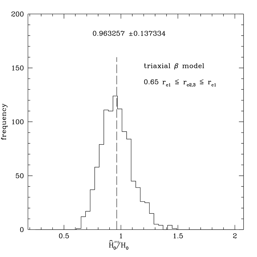
Figure 2.— The distributions of $\hat{H}_{0}^{\rm avg}$, inferred from the clusters by averaging major and minor axes, compared to the assumed value of $H_{0}$, for the optimal sample. The distribution mean values are indicated by dashed lines (value of sample means and deviations above lines).

References

- (1)
- (2) Anninous, P. & Norman, M.L., 1996, ApJ, 459, 12
- (3) Birkinshaw, M. 1998, Physics Reports, in press
- (4) Birkinshaw, M., 1979, MNRAS, 187, 847
- (5) Buote, D.A., & Canizares, C.R., 1996, ApJ, 457, 565
- (6) Burns, J.O., 1990, AJ, 99, 14
- (7) Calstrom, J.E., Joy, M. K. & Grego, L. 1996, ApJ, 456, L75
- (8) Cavaliere, A., Danese, L. & De Zotti, G., 1979, A&A, 75, 322
- (9) Cavaliere, A. & Fusco-Femiano, R., 1978, A&A, 70, 677
- (10) Cooray, A.R., 1998, A&A, in press, astro-ph 9808186
- (11) Edge, A.C., Stewart, G.C., Fabian, A.C., & Arnaud, K.A., 1990, MNRAS, 239, 559
- (12) Grainge, K., Jones, M., Pooley, G. Saunders, R., Baker, J., Haynes, T. & Edge, A., 1996, MNRAS, 278, L17
- (13) Gunn, J.E., 1978, In Observational Cosmology 1; eds Maeder, A., Martinet, L. & Tammann, G.; (Sauverny: Geneva Observatory)
- (14) Hughes, J.P., 1997, in Proceedings IAU 188 ”The Hot Universe”, astro-ph/9711135
- (15) Hughes, J.P. & Birkinshaw, M. 1998, ApJ, in press, astro-ph/9801183
- (16) Inagaki, Y., Suginohara, T. & Suto, Y. 1995, PASJ, 47, 411
- (17) McMillan, S.L.W., Kowalski, M.P. & Ulmer, M.P., ApJS, 70, 723
- (18) Metzler, C. A. & Evrard, A. E., 1997, astro-ph 9710324
- (19) Mohr, J.J., Mathiesen, B., and Evrard, A.E., 1999, ApJ, in press, astro-ph/9901281
- (20) Mohr, J.J., Evrard, A.E., Fabricant, D.G. & Geller, M.J., 1995, ApJ, 447, 8
- (21) Myers, S.T., Baker, J.E., Readhead, A.C.S., & Leitch, E.M., 1997, ApJ, 485, 1
- (22) Neumann, D.M, & Arnaud, M., 1999, astro-ph/9901092
- (23) Peres, C.B., Fabian, A.C., Edge, A.C., Allen, S.W., Johnstone, R.M., & White D.A., 1998, MNRAS, 298, 416
- (24) Roettiger, K., Stone, J.M. & Mushotsky, R.F. 1997, ApJ, 482, 588
- (25) Sarazin, C. 1986, Rev. Mod. Phys., 58, 1
- (26) Silk, J.I. & White, S.D.M., 1978, ApJ, 226, L3
- (27) Sunyaev, R.A. & Zel’dovich, Y.A. 1972, Comm. Astrophys. Sp. Phys., 4, 173
- (28) Thomas, P. A., Colberg, J.M., Couchman, H.P., Efstathiou, G.P., Frenck, C.S., Jenkins, A.R., Nelson, A.H., Hutchings, R.M., Peacock, J.A., Pearce, F.R. & White, S.D.M. 1998, MNRAS, 296, 1061
- (29) White, D.A., Jones, C., & Forman, W., 1997, MNRAS, 292, 419
- (30) Van Speybroeck, L. & Vikhlinin, A., 1997, private communication
- (31)