DESY 99-18

V.A.Balkanov², I.A.Belolaptikov⁷, L.B.Bezrukov¹, N.M.Budnev², A.G.Chensky²,
I.A.Danilchenko¹, Zh.-A.Djilkibaev¹, G.V.Domogatsky¹, A.A.Doroshenko¹,
S.V.Fialkovsky⁴, O.N.Gaponenko¹, A.A.Garus¹, T.I.Gress², A.Karle^8,∗, A.M.Klabukov¹,
A.I.Klimov⁶, S.I.Klimushin¹, A.P.Koshechkin¹, V.F.Kulepov⁴, L.A.Kuzmichev³, S.Lovzov²,
B.K.Lubsandorzhiev¹, T.Mikolajski⁸, M.B.Milenin⁴, R.R.Mirgazov², A.V.Moroz²,
N.I.Moseiko³, S.A.Nikiforov², E.A.Osipova³, D.Pandel^8,∗∗, A.I.Panfilov¹, Yu.V.Parfenov²,
A.A.Pavlov², D.P.Petukhov¹, P.G.Pokhil¹, P.A.Pokolev², E.G.Popova³, M.I.Rozanov⁵,
V.Yu.Rubzov², I.A.Sokalski¹, Ch.Spiering⁸, O.Streicher⁸, B.A.Tarashansky², T.Thon⁸,
R.Wischnewski⁸, I.V.Yashin³

1 - Institute for Nuclear Research, Russian Academy of Science (Moscow),
2 - Irkutsk State University (Irkutsk),
3 - Moscow State University (Moscow),
4 - Nizhni Novgorod State Technical University (Nizhni Novgorod),
5 - St.Petersburg State Marine Technical University (St. Petersburg),
6 - Kurchatov Institute (Moscow),
7 - Joint Institute for Nuclear Research (Dubna),
8 - DESY-Zeuthen (Zeuthen)
** - now at University of Wisconsin (USA)       ** - now at University of Irvine (USA)

Abstract

We present results of an experiment performed in Lake Baikal at a depth of about 1 km. The photomultipliers of an underwater neutrino telescope under construction at this site have been illuminated by a distant laser. The experiment not only provided a useful cross-check of the time calibration of the detector, but also allowed to determine inherent optical parameters of the water in a way complementary to standard methods. In 1997, we have measured an absorption length of 22 m and an asymptotic attenuation length of 18 m. The effective scattering length was measured as 480 m. Using $\langle\cos\theta\rangle=0.95(0.90)$ for the average scattering angle, this corresponds to a geometrical scattering length of 24 (48) m.

submitted to APPLIED OPTICS

1 Introduction

Propagation of light in optical media is governed by two basic phenomena: absorption and scattering. In the first case the photon is lost, in the second case it changes its direction. The inherent parameters generally chosen as a measure for these phenomena are the absorption length $\lambda_{abs}$, the scattering length $\lambda_{sct}$ and the scattering function (or scattering tensor if polarization is taken into account) $\beta\left(\theta\right)$.

The determination of optical parameters for the water of deep lakes or oceans meets considerable problems. Typical values for $\lambda_{abs}$ in the window of maximum transparency are about 20 m for clearest water in deep lakes [1, 2, 3] and 50 m for deep oceans [4, 5, 6]. Another important property of natural water is the strongly forward peaked scattering, with $\left\langle\,\cos\ \theta\,\right\rangle$ = 0.85 – 0.96 in oceans [7] or lakes [3, 8, 9] and scattering lengths of 10 – 50 m. Because of the long absorption and scattering lengths and the steep scattering function, devices to measure these optical parameters in clear water have to be extremely precise and well calibrated.

In vitro measurements suffer from the comparatively short base length of the laboratory devices and from the fact that the samples of the medium can deteriorate before being analyzed in laboratory. Furthermore, for in vitro measurements it is rather difficult to perform long-term experiments and to observe seasonal variations of the optical parameters. In situ devices are difficult to handle, particularly for greater depths. On the other hand, only in situ measurements allow long term observations of the medium, including the implications of temporary changing mechanical, chemical, biological and thermal conditions.

In the course of preparing a deep-underwater neutrino telescope in Lake Baikal, in situ optical measurements have been carried out over several years. We have constructed a special device (see [1, 10]) and developed proper methods [3, 8, 9] to determine and to monitor the hydro-optical parameters of the water body at the site of Baikal Neutrino Telescope. The data obtained from these measurements do not only yield necessary input parameters for the operation of the telescope, but are interesting as well for environmental science.

In this paper we present the results of optical measurements obtained in a way complementary to standard limnological (oceanological) methods, using a laser as light source and an underwater neutrino telescope as light detector. This kind of telescope represents a new class of giant instruments coming into operation at various locations in deep oceans and lakes [11], and even in glaciers [12]. Being permanently operational over several years, underwater telescopes can perform, as a by-product and for calibration purposes, measurements of optical parameters as well as of water currents, bioluminescence etc.

We have measured the spatial and temporal distribution of monochromatic light from a pulsed isotropic, point-like source. From the analysis of the spatial distribution, we derive the values for absorption length $\lambda_{abs}$ and for the so-called asymptotic attenuation length $\lambda_{asm}$. From the time delay of the short light flashes arriving at the photomultipliers of the telescope, we derive $\lambda_{eff}$, which is an effective parameter describing scattering.

We describe the Baikal Neutrino Telescope in section 2, and the laser experiments to determine the optical parameters of the water in section 3. In section 4 we derive the expressions for the light field as a function of the distance to an isotropic source. The experimental data are analyzed in section 5, and values for parameters characterizing absorption and scattering are derived. Section 6 contains the conclusion.

2 The Baikal Neutrino Telescope

The Baikal Neutrino Telescope [13, 14] exploits the deep water of the Siberian lake as a detection medium for secondary charged particles, like muons or electrons, generated in neutrino interactions. Neutrinos are etheric particles characterized by their extremely rare interaction with all kind of matter. They are supposed to be generated in cosmic particle accelerators like the nuclei of Active Galaxies or binary star systems. Shielded by kilometers of water burden, underwater telescopes aim to detect the rare reactions of neutrinos from these exotic sources.

A lattice of photomultiplier tubes (PMTs) spread over a large volume records the Cherenkov light emitted by the relativistic charged particles. The light arrival times at the locations of the PMTs are measured with an accuracy of a few nanoseconds. From the time pattern, the particle trajectory can be reconstructed with a resolution of 1 – 2 degrees. In addition to the arrival times, the amplitudes of the signals are recorded. Typical amplitudes for particles triggering the array are in the few-photoelectron range.

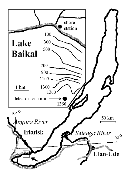
Figure 1: Location of the Baikal experiment

The Neutrino Telescope NT-200 is being deployed in the southern part of Lake Baikal (fig.1). The distance to shore is 3.6 km, the depth of the lake is 1366 m at this location. Fig.2 sketches the instrumentation of the site. Strings anchored by weights at the bottom are held in vertical position by buoys at various depths. The deployment of the detector elements is carried out in late winter, when the lake is covered by a thick layer of ice. Three cables (1,2,3 in fig.2) connect the detector with the shore station. Each shore cable ends at the top of a string (4,5,6, respectively). String 7 carries the telescope. A special ”hydrometric” string 8 is equipped with instruments to measure the optical parameters of the water as well as water currents, temperature, pressure and sound velocity. The spatial coordinates of the components of the telescope are monitored by an ultrasonic system consisting of transceivers 9-14, and receivers along the strings. The relative coordinates of the components are determined with an accuracy of about 20 cm.

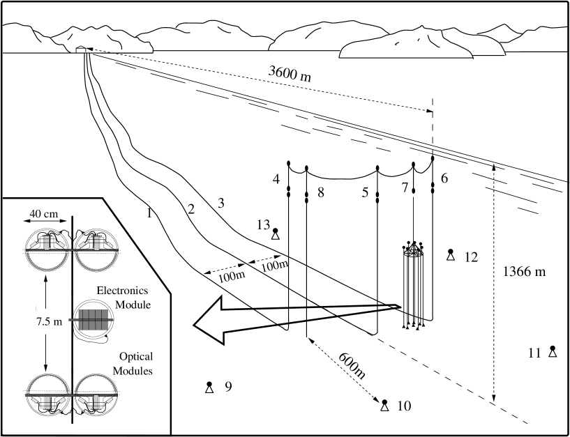
Figure 2: Overall view of the NT-200 complex. 1,2,3 – cables to shore, 4,5,6 – string stations for shore cables 7 – string with the telescope, 8 – hydrometric string, 9-14 – ultrasonic emitters. The detail bottom left shows two pairs of optical modules (OMs), together with the electronics module controlling the OMs. Shown are two pairs directed face to face.

The telescope NT-200 consists of 8 sub-strings arranged at the center and the edges of an equilateral heptagon. The light detection elements are optical modules (OMs) containing a hybrid phototube Quasar-370 with a hemispherical photocathode of 370 mm diameter. The time resolution of the Quasar-370 is 3 nsec for a single-photoelectron signal and improves to about 1 nsec for large amplitudes. The OMs are arranged pairwise, with the two phototubes being operated in coincidence (see fig.2). If an event triggers at least 3 pairs within 500 nsec, light arrival time and amplitude of each hit pair (”channel”) are recorded. Each of the 8 strings of NT-200 will carry 24 OMs.

The time calibration is performed with a help of a nitrogen laser positioned just above the array [16]. The 1-nsec light flashes of the laser are transmitted by optical fibers of equal length to each of the OM pairs.

3 The Laser Experiments

For the two experiments described in this paper, an additional laser device was operated at various locations with respect to the PMTs of the neutrino telescope. Short light pulses were emitted by the laser, traveled through the water, and were detected by the PMTs during normal operation, when the standard trigger on muons crossing the array (3-fold coincidence within 500 ns) was set.

The laser module [16] contains a pulsed nitrogen laser (wavelength 337.1 nm) which pumps a dye laser with an emission maximum at 475 nm. This wavelength well matches the point of maximum transparency at 490 nm, where Baikal water has an absorption length of about 20 m.

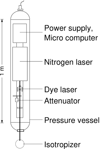
Figure 3: Schematic view of the laser module

The light pulses generated by the laser have a length of about 0.5 ns (FWHM), thus being shorter than the time resolution of the photomultipliers. An attenuation disk, moved by a stepper motor, is used to attenuate the light beam in five steps from 100 % to 0.3 % of the laser intensity of about $10^{12}$ photons per pulse. Both lasers, the attenuator, power supplies and a micro-computer are contained in a glass pressure vessel [18] of 155 mm diameter and 1 m length (see fig.3). After having crossed the vessel wall, the laser beam is directed into a hollow sphere with a diffusely reflecting inner surface. Through small holes in the sphere the light is able to escape, with a nearly isotropic distribution. Due to the large distance to the detector, the laser module can be considered as an isotropic point-like light source.

The laser can be triggered to generate cycles of light pulses. Each cycle consists of 5 series of 200 equally intense pulses. The intensities of consecutive series differ by a factor of 3 to 4. Laser-induced events fulfill the trigger conditions for muons crossing the array. They can be separated from those using the periodicity of the laser pulses (9.1 Hz). The remaining background from muon events ranges from $10^{-3}$ for low light intensities to $10^{-4}$ for higher intensities.

In the following, data taken with 2 configurations are analyzed:

• 1995 experiment

  In April 1995, an intermediate version of the final array NT-200 was deployed. It carried 72 optical modules mounted at four short and one long string (see fig.4). The laser experiment has been performed immediately after deployment of this detector (NT-72). The laser module was deployed from the ice surface and placed at several locations 20 to 200 m away from the PMTs. Preliminary results from this experiment have been published in [17].

  

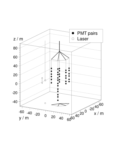
  Figure 4: Schematic view of the 1995 configuration of the laser experiment. Each filled circle represents a pair of optical modules (channel). The laser is indicated by the open circle.

• 1997 experiment

  The 1997 laser experiment was performed after having deployed the first string of the 1997 season. The string carried 24 PMTs, with the highest at 1059 m depth and the lowest at 1128 m depth. The laser was moved along the string at a horizontal distance of 12 meters to the string with the PMTs, starting at a height close to the top PMT. The last of the 15 positions was 221 m below the first, at 1286 m (see fig.5).

In both experiments, the times and amplitudes of the fired channels were recorded if the standard trigger on muons crossing the array (3-fold coincidence within 500 ns) was fulfilled.

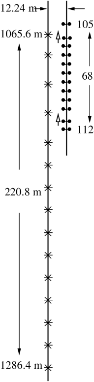
Figure 5: Schematic view of the the 1997 configuration of the laser experiment. Channels are shown explicitly as pairs of OMs. The various positions of the laser are indicated by stars. The OMs face down, with the exception of channels 2 and 11 (upward arrows) which are directed upward.

4 The light field of an isotropic source in a medium

The photon field $\Phi\left(R,\,\vec{\Omega},\,t\right)$ produced in a medium by a pulsed point-like source of monochromatic light is a function of distance $R$ from the light source, direction vector $\vec{\Omega}$, and time $t$ after emission. This function can be calculated by Monte Carlo methods, with $\lambda_{abs}$, $\lambda_{sct}$ and $\beta\left(\theta\right)$ as input parameters. In this section we derive analytical approximations for the photon field and compare it to the results of Monte Carlo simulations.

In the special case of a medium without scattering one has

$$\Phi\left(R,\,\vec{\Omega},\,t\right)=F\left(R\right)\delta\left(\vec{\Omega}\right)\delta\left(t-R/v\right),$$ (1)

where $F(R)$ is the photon flux:

$$F\left(R\right)=\int\,\Phi\left(R,\,\vec{\Omega},\,t\right)\,d\vec{\Omega}\,dt=\frac{I_{0}}{4\pi R^{2}}\,e^{-\frac{R}{\lambda_{abs}}}.$$ (2)

For a medium with scattering, $F\left(R\right)$ can be written as

$$F\left(R\right)=\frac{I_{0}}{4\pi R^{2}}\,e^{-\frac{R}{\lambda_{abs}}\,\mu\left(R\right)},$$ (3)

where, in the general case, $\mu\left(R\right)$ is some intricate function of $R$. This function takes into account the increase of the photon path due to scattering. It was shown in [20] that $1<\mu\left(R\right)<1.01$ for distances $R<0.6\,\lambda_{sct}$ and steep scattering functions ($\left\langle\cos\,\theta\right\rangle\geq 0.9$). At larger distances, however, the contribution from scattering becomes significant. In the following we estimate the influence of scattering on the photon flux at moderate distances from the source.

Due to scattering, a photon does not travel along a straight line but follows some polygonal path with random vectors $\vec{r}_{i}$ ($i=1,\ 2,\ ...\,n$) which are the trajectories of a photon between two successive scattering acts. Thus,

$$\left\langle r_{i}\right\rangle=\lambda_{sct},$$ (4)

$$\left\langle\vec{r}_{i}\cdot\vec{r}_{i+1}\right\rangle=\lambda_{sct}^{2}\,\left\langle\cos\,\theta\right\rangle.$$ (5)

It turns out that under rather general assumptions about the shape of the scattering function, the following relation takes place:

$$\left\langle\cos\,\theta_{i\,,\,i+k}\right\rangle=\left\langle\cos\,\theta\right\rangle^{k},$$ (6)

where $\theta_{i\,,\,i+k}$ is the angle between the vectors $\vec{r}_{i}$ and $\vec{r}_{i+k}$. In this case

$$R=\sqrt{\sum\limits_{i=1}^{n}\sum\limits_{j=1}^{n}\left\langle\vec{r}_{i}\cdot\vec{r}_{j}\right\rangle}=\lambda_{sct}\sqrt{n+2\sum\limits_{i=1}^{n}\left(n-k\right)\left\langle\cos\,\theta\right\rangle^{k}}.$$ (7)

The average length $L$ of the photon path for $n$ successive scattering acts is

$$L=n\cdot\lambda_{sct}.$$ (8)

For simplicity we consider the case of $\left\langle\cos\,\theta\right\rangle$ close to 1. With $\left(1-\left\langle\cos\,\theta\right\rangle\right)$ being small, from from eqs.(7) and (8) one gets

$$L\left(R\right)\approx R\sqrt{1+\frac{1}{3}\frac{R}{\lambda_{sct}}\,\left(1-\left\langle\cos\,\theta\right\rangle\right)}.$$ (9)

For water with strongly forward peaked scattering we finally obtain

$$F\left(R\right)=\frac{I_{0}}{4\pi R^{2}}\,e^{-\frac{R}{\lambda_{abs}}\,\sqrt{1+\frac{1}{3}\frac{R}{\lambda_{sct}}\,\left(1-\left\langle\cos\,\theta\right\rangle\right)}}.$$ (10)

We note that in this equation $\lambda_{sct}$ and $\left\langle\cos\,\theta\right\rangle$ are combined in an expression $\lambda_{sct}/(1-\langle\cos\theta\rangle)$, resulting in a reduction of the number of independent parameters in eq. (10) from three to two. This agrees with the conclusions drawn in [21] from the measurements of the photon flux of an isotropic source in artificial media as well as in natural water. For all these strongly forward scattering media it was found that $F\left(R\right)$ can be described as a function of only two parameters, $\lambda_{abs}$ and $P$, where

$$P=\frac{\lambda_{abs}}{\lambda_{sct}}\,\frac{\left\langle\theta^{2}\right\rangle}{2}.$$ (11)

Since for $\left\langle\cos\,\theta\right\rangle\simeq 1$ one has $\left\langle\theta^{2}\right\rangle\approx 2\left(1-\left\langle\cos\,\theta\right\rangle\right)$, eq.(10) can be rewritten in terms of the parameters $\lambda_{abs}$ and $P$ (see also [23, 24]):

$$F\left(R\right)=\frac{I_{0}}{4\pi R^{2}}\,e^{-\frac{R}{\lambda_{abs}}\,\sqrt{1+\frac{1}{3}\frac{R}{\lambda_{abs}}\,P}}.$$ (12)

Our Monte Carlo simulations [22] confirm the results of [21] which proved for an interval $\langle\theta^{2}\rangle$ = 0.114 to 0.582 and for distances $R<5\,\lambda_{abs}$ that the error in $F(R)$ resulting from the reduction of $\lambda_{scatt}$ and $\beta(\theta)$ to $P$ is smaller than than $1\%$.

With the notation

$$\lambda_{eff}=\frac{\lambda_{sct}}{1-\left\langle\cos\,\theta\right\rangle},$$ (13)

eq.(10) can be written as

$$F\left(R\right)=\frac{I_{0}}{4\pi R^{2}}\,e^{-\frac{R}{\lambda_{abs}}\,\sqrt{1+\frac{1}{3}\frac{R}{\lambda_{eff}}}}.$$ (14)

The definition of $\lambda_{eff}$ according to eq.(13) coincides with the one for the diffusion case provided $\left\langle\cos\,\theta\right\rangle$ is close to zero (i.e. quasi-isotropic scattering) and in the expansion in powers of $\left\langle\cos\,\theta\right\rangle$ only the first correction term is taken into account. We emphasize that in our case $\lambda_{eff}$ is just a convenient, artificial parameter (comparable, e.g., to the parameter $P$ in eq. (12)) and should not be associated with an ”effective” increase of the scattering length due to the anisotropy of the scattering.

Although eq.(14) was derived here for strongly forward peaked scattering functions, similar considerations can be also performed for the case where $\left\langle\cos\,\theta\right\rangle$ is not close to unity as, for instance, in glacier ice which is exploited for the AMANDA neutrino telescope [12, 25].

Eq.(12) may also be considered as a particular solution of the transport equation for the small-angle approximation. In the framework of the small-angle approximation the general solution has the form (see e.g. [26]):

$$F\left(R\right)=\frac{I_{0}}{4\pi R^{2}}\,\frac{\left(R\,\sqrt{P}/\lambda_{abs}\right)}{\sinh\left(R\,\sqrt{P}/\lambda_{abs}\right)}\,e^{-\frac{R}{\lambda_{abs}}}.$$ (15)

Eq.(12) can be formally found from the solution (15) by expansion with respect to the small parameter $R\,\sqrt{P}/\lambda_{abs}$. The opposite case, $R\,\sqrt{P}/\lambda_{abs}\gg 1$, gives

$$\begin{array}[]{c}F\left(R\right)=\frac{I_{0}\sqrt{P}}{2\pi R\lambda_{abs}}\,e^{-\frac{R}{\lambda_{abs}}\left(1+\sqrt{P}\right)}=\\ \\ =\frac{I_{0}}{2\pi R\sqrt{\lambda_{abs}\lambda_{eff}}}\,e^{-\frac{R}{\lambda_{abs}}\left(1+\sqrt{\lambda_{abs}/\lambda_{eff}}\right)}.\end{array}$$ (16)

In fig.6 we compare the results of our Monte Carlo simulations (histogram) with the predictions of eq.(12) (dashed line) and eq.(15) (solid line) for $\lambda_{abs}=23$ m and $P=0.1$. The dotted line represents the result of eq.(3) with $\mu\left(R\right)=1$ (the case without scattering). One observes a perfect agreement of the approximation (15) with the Monte Carlo calculations over a wide region of distances. For not too large distances also eq.(12) agrees with the MC data.

In next section we will apply the expressions obtained to the experimental data.

Figure 6: Intensity vs. distance as obtained from Monte Carlo calculations (histogram), eq.(12) (dashed line) and eq.(15) (solid line). In all three cases $\lambda_{abs}$=23 m and $P=0.1$ have been used. The dotted line is the result of eq.(3) with $\mu(R)=1$

5 Analysis of experimental data

5.1 Absorption

1995 experiment

The absorption of light on its way to the photomultipliers can be determined from the measured amplitudes. For the 1995 laser experiment, 24 of the 72/2 = 36 channels have been included in the analysis. The combination of amplitudes from different photomultipliers requests a careful calibration. After amplitude calibration, and using the well-known angular acceptance of the photomultipliers, the mean amplitudes measured by each channel of NT-72 have been converted to light intensities. In fig.7 the dependence of the photon density on the laser distance is shown. The points represent the measured signals from the optical modules facing toward the laser, for different laser positions and intensities. The data are well described by the relation

$$F(R)\sim\frac{1}{R^{2}}\,e^{-\frac{R}{\lambda}}$$ (17)

over a wide region of distances $R$. This is the approximation of equation(14) for the case $R/\left(3\lambda_{eff}\right)\ll 1$. With $\lambda_{eff}\approx 480$ m (see sect.5.2) and $R$ covering the range 30 – 150 m, the latter condition is satisfied. Therefore, $\lambda$ in eq.(17) can be identified with the absorption length $\lambda_{abs}$. The value of $\lambda_{abs}$ obtained from the experimental data of 1995 is $(19.9\pm 0.2$) m [17].

Figure 7: Laser experiment 1995: Light intensity as a function of distance to the laser. The dots show the measured values, the solid line shows an exponential decrease with $\lambda$ = 19.9 m. If scattering is included, the dependence shown by the dashed line is expected.

1997 experiment

In fig.8 we present the average amplitudes multiplied with $R^{2}$ vs. distances $R$, for one of the channels of the first 1997 telescope string. The data points can be grouped along five straight lines, each corresponding to a given intensity of the laser. Contrary to the experiment of 1995, the analysis has been performed for each channel separately. This procedure avoids biases due to possible errors in the relative amplitude calibration of the PMTs. The large number of channels (i.e the multiple independent determination of $\lambda_{abs}$) and the high precision of the measured amplitudes and distances results in small errors of $\lambda_{abs}$. The absorption length is $\lambda_{abs}=22$ m, with variations of about $6\%$, dependent on the covered range in $R$. Most of this variation (about $5\%$) is due to the change of $\lambda_{abs}$ with depth. The errors of the measurement itself are estimated to be smaller than $1\%$ (i.e. 0.2 m). We attribute the discrepancy between 1995 and 1997 results to time variations of the water parameters.

Figure 8: Laser experiment 1997: Logarithm of average amplitude $\langle A\rangle$ times squared distance $R^{2}$ versus distance $R$ for one of the 12 channels of the first string. Curves are to guide the eye. Each curve corresponds to one of the five different laser intensities. Saturation of the curves at low $R$ is due to the limited dynamical range, flattening at high $R$ is due to the noise. Fits have been applied to the linear part of the curves.

5.2 Scattering

To investigate scattering we evaluated the delay in arrival times of the photons. According to eqs.(9), (13), these times can be written as

$$t=\frac{R}{c_{w}}\,\sqrt{1+\frac{1}{3}\frac{R}{\lambda_{eff}}}\approx\frac{1}{c_{w}}\,\left(R+\frac{1}{6}\frac{R^{2}}{\lambda_{eff}}\right),$$ (18)

where $c_{w}$ is the velocity of light in water. Note that this approximation applies only for multiple scattering under small angles. Strongly scattered photons (e.g. due to Rayleigh scattering) arrive much later and would not coincide with one of the many forward scattered photons. This, however, is a condition for a channel to trigger, since its two OMs are operated in coincidence. Eq.(18) does not include effects of absorption. Consequently, in reality the average time delay is smaller than given by expression (18): photons traveling a longer path are absorbed and contribute less to the average delay. Absorption is described by the exponential probability distribution of eq.(14).

With $\lambda_{abs}$ determined from the intensity-vs.-distance curve, the effect of absorption can be subtracted from the experimental data as well as from Monte Carlo data. Fig.9 compares the experimental delays to delay curves expected from different assumptions on $\lambda_{eff}$. For both experiment and prediction the effect of absorption is subtracted so that eq.(18) can be applied. The solid line gives the best fit and corresponds to $\lambda_{eff}=480$ m. The error of $\lambda_{eff}$ is estimated as 15%.

Figure 9: Laser experiment 1997: Average arrival times $\langle t\rangle$ vs. distance $R$. Dots represent the measured values, lines give the expectations for different values of the effective scattering length $\lambda_{eff}$. In both cases absorption effects have been subtracted (see text).

The value of $\lambda_{eff}$ obtained in the present work can be compared with the results of the direct measurements of $\lambda_{sct}$ and $\beta\left(\theta\right)$ cited in [3, 9]. There, with the help of the measured scattering function $\beta\left(\theta\right)$, $\left\langle\cos\left(\theta\right)\right\rangle\approx$ 0.95 – 0.96 was found. For $\lambda_{sct}$ values of 15 – 18 m have been obtained. In 1997 (not published), we measured $\left\langle\cos\left(\theta\right)\right\rangle\approx$ 0.9 and $\lambda_{sct}=$ 40–50 m. With eq.(13), this results in $\lambda_{eff}$ = 300 – 450 m and $\lambda_{eff}$ = 400 – 500 m (1997), compatible with $\lambda_{eff}=480\pm 70$ m determined in the present analysis. We note that for $\left\langle\cos\left(\theta\right)\right\rangle$ close to $1$ the result is extremely sensitive to the exact value of $\left\langle\cos\left(\theta\right)\right\rangle$. Also, scattering parameters in Lake Baikal are known to vary strongly with time (see [27]). This makes the agreement even more satisfactory.

5.3 Asymptotic attenuation length

As follows from eq.(16), at large distances

$$F\left(R\right)\sim\frac{1}{R}\,e^{-\frac{R}{\lambda_{asm}}},$$ (19)

where

$$\lambda_{asm}=\frac{\lambda_{abs}}{1+\sqrt{\lambda_{abs}/\lambda_{eff}}}$$ (20)

is the so-called asymptotic attenuation length. Eq.(16) describes the asymptotic behavior of $F\left(R\right)$. In the asymptotic regime, angular and spatial dependences of $\Phi\left(R,\,\vec{\Omega},\,t\right)$ can be factorized (see, for example, [28]) so that

$$\int\,\Phi\left(R,\,\vec{\Omega},\,t\right)\,\,dt=F\left(R\right)\rho\left(\vec{\Omega}\right).$$ (21)

Therefore, the measurement of $\lambda_{asm}$ is not sensitive to the orientation of the PMTs and can be performed independently for various directions.

Although expression (16) follows from eq.(15) only for very large distances, our Monte Carlo simulations show that the $e^{-\frac{R}{\lambda_{asm}}}/R$ behavior is already seen for $R\approx 100$ m if $\lambda_{abs}\approx 20$ m, $\lambda_{eff}\leq 500$ m and the channel faces away from the light source. Photons observed by these channels are preferently very often scattered and form a light field close to the asymptotic propagation regime. Thus the value of $\lambda_{asm}$ can be evaluated from the data of the 1997 laser experiment where the maximal distance $R$ was approximately 180 m. In fig.10 the $R$ dependence of the amplitudes for channel $N^{\underline{0}}\,2$, looking away from the source, is shown. The experimental data behave exponentially with an exponent $1/L_{\uparrow}\approx 1/(17.6\pm 0.5)$ m^-1.

Figure 10: Logarithm of the product of average amplitude $\langle A\rangle$ and $R$ versus distance $R$ in the ”asymptotic” regime for channel 2, looking away from the laser.

Comparing Monte Carlo simulations to eq.(15) we found that in the general case $0.95\cdot L_{\uparrow}\leq\lambda_{asm}\leq 1.05\cdot L_{\uparrow}$, and so we finally obtain $\lambda_{asm}$ = (17.6 $\pm$ 1.5) m.

Since there is a certain overlap between the regions in which both eq.(19) and eq.(14) describe the photon flux as a function of distance, one could try to estimate $\lambda_{eff}$ from $\lambda_{asm}$ and $\lambda_{abs}$, using eq.(20). Unfortunately, the final result is very sensitive to the exact values of asymptotic and absorption length (cf. what was said above on the estimation of $\lambda_{eff}$ from $\left\langle\cos\left(\theta\right)\right\rangle$). Therefore, the available accuracy of our experiments does not allow yet to determine $\lambda_{eff}$ in this way. However, $\lambda_{asm}$ itself can be applied as a useful parameter for the description of the photon flux at large distances.

6 Conclusions

We have used a neutrino telescope triggered by laser light pulses to measure the optical properties of clear, open water with high accuracy. For 1 km deep water in Lake Baikal, in 1997 we determined an absorption length of $22.0\pm 1.2$ m and an asymptotic attenuation length of $17.6\pm 1.5\,$m. Quite different to standard methods, the effective scattering length was obtained from nanosecond timing measurements. It was measured as $480\pm 70$ m which under the assumption of $\langle\cos\theta\rangle$ = 0.95 (0.9) translates to a geometrical scattering length of 24 (48) m.

In future, we want to refine these measurements using a larger number of optical modules and measuring over an extended range of distances between optical modules and laser. Also, we plan a continuous monitoring of the optical parameters over the full year.

This work was supported by the RFFI grant 97-05-96466.

References

- [1] L.B.Bezrukov et al., Measurement of the light absorption coefficient in Lake Baikal water, Oceanology, 30 (1990) 1022 (in Russian).
- [2] L.B.Bezrukov et al., Titel, Proc. 2nd Symp. on Marine and Atmospheric Optics, Krasnojarsk 1990, 2 (in Russian) 10.
- [3] O.N.Gaponenko et al., Reconstruction of the primary hydrooptical characteristics from the light field of a point source, Atmosph. Oceanic Optics 9 (1996) 677.
- [4] J.R.Zaneveld, Optical Properties of the Keahole-DUMAND Site, 1980 International DUMAND Symposium, ed. V.J.Stenger, Hawaii 1980, 1,1.
- [5] H.Bradner, G. Blackinton, Long baseline measurements of light transmission in clear water, Appl. Optics 23 (1984) 1009.
- [6] E.G.Annasontzis et al., Measurement of light transmissivity in clear and deep sea water, Nucl. Instr. Meth. A349 (1994) 242.
- [7] N.G.Jerlov, Marine Optics, Elsever Oceanography Series, 5 (1976).
- [8] O.N.Gaponenko et al., Calculation of the scattering function from the light field of a point like isotropic source, Proc. 1st Symp. on Atmosph. Oceanic Optics, Tomsk 1994, 1, 90 (in Russian).
- [9] B.A.Tarashchanskii et al., On a technique for measuring the scattering phase function using the light field from a source with a wide directional pattern, Atmosph. Oceanic Optics 7 (1994) 819.
- [10] B.A.Tarashchanskii et al., Stationary deep-water meter of hydrooptical parameters, Atmosph. Oceanic Optics 8 (1995) 771.
- [11] F.Halzen, Large Natural Cherenkov Detectors: Water and Ice, Proc. 5th Int.Workshop on Topics in Astroparticle and Underground Physics, Gran Sasso 1997, hep-ex/9801009.
- [12] S.Barwick et al., Amanda Status Report, Proc. 25th ICRC (Durban 1997) 7, 1.
- [13] I.A.Belolaptikov et al., The Baikal Underwater Neutrino Telescope: Design, Performance and First Results, Astroparticle Physics 7 (1997) 263.
- [14] I.A.Sokalski and Ch.Spiering (eds.), The Baikal Neutrino Telescope NT-200, BAIKAL Note 92-03 (1992).
- [15] Ch.Spiering for the Baikal Collaboration, The Baikal Deep Underwater Neutrino Experiment: Results, Status, Future, Proc.Int.School of Nuclear Physics,Erice 1997,astro-ph/9801044.
- [16] Th.Mikolajski, PhD Thesis, Berlin 1995 (in German)
- [17] I.A.Belolaptikov et al., Response of the NT-36 Array to a Distant Point-Like Light Source, Proc. 24th Int. Cosmic Ray Conference, Rome 1995, 1043.
- [18] VITROVEX Deep Sea Instrument Housings, Nautilus Marine Service, Bremen, Germany.
- [19] D.Pandel, Diploma Thesis, Berlin 1996.
- [20] D.Bauer, J.C.Brun-Cottan, A.Saliot, Princip d’une measure directe dans l’eau de mer du coefficient d’absorption de la lumiere, Cah. Occeanogr. 23 (1971) 841.
- [21] V.N.Pelewin, T.M.Prokudina, Determination of the absorption coefficient of sea water by the parameters of an isotropic source, Atmosph. Oceanic Optics (1972).
- [22] O.Ju.Lanin, Diploma Thesis, Moscow 1989.
- [23] V.I.Dobrynin et al., Spectral light absorption by deep Baikal water, Atmosph. Oceanic Optics 10 (1997) 234.
- [24] L.S.Dolin, Dokladi Akademii Nauk 8 (1981) 1344.
- [25] The Amanda Collaboration, Science 267 (1995) 1147.
- [26] A.S.Monin, Oceanic Optics, Vols. 1 and 2 , 1983.
- [27] P.P.Sherstiankin, Baikal Frontogenesis from the optical observation data, Rep. of U.S.S.R. Academy of Sciences 326 (1992) 366 (in Russian).
- [28] L.S.Dolin, On a technique for calculation of the brightness at large optical distances from a light source, Bull. of U.S.S.R. Academy of Sciences, FAO, Vol. 17, No.1 (1981) 102 (in Russian).