The Nature of Galaxy Bias and Clustering

Abstract

We have used a combination of high resolution cosmological N-body simulations and semi-analytic modelling of galaxy formation to investigate the processes that determine the spatial distribution of galaxies in cold dark matter (CDM) models and its relation to the spatial distribution of dark matter. The galaxy distribution depends sensitively on the efficiency with which galaxies form in halos of different mass. In small mass halos, galaxy formation is inhibited by the reheating of cooled gas by feedback processes, whereas in large mass halos, it is inhibited by the long cooling time of the gas. As a result, the mass-to-light ratio of halos has a deep minimum at the halo mass, $\sim 10^{12}M_{\odot}$, associated with $L_{*}$ galaxies, where galaxy formation is most efficient. This dependence of galaxy formation efficiency on halo mass leads to a scale-dependent bias in the distribution of galaxies relative to the distribution of mass. On large scales, the bias in the galaxy distribution is related in a simple way to the bias in the distribution of massive halos. On small scales, the correlation function is determined by the interplay between various effects including the spatial exclusion of dark matter halos, the distribution function of the number of galaxies occupying a single dark matter halo and, to a lesser extent, dynamical friction. Remarkably, these processes conspire to produce a correlation function in a flat, $\Omega_{0}=0.3$, CDM model that is close to a power-law over nearly four orders of magnitude in amplitude. This model agrees well with the correlation function of galaxies measured in the APM survey. On small scales, the model galaxies are less strongly clustered than the dark matter, whereas on large scales they trace the occupied halos. Our clustering predictions are robust to changes in the parameters of the galaxy formation model, provided only those models that match the bright end of the galaxy luminosity function are considered.

1 Introduction

Studies of the clustering of cosmological dark matter have progressed enormously in the past twenty years. The dynamical evolution of the dark matter is driven by gravity and fully specified initial conditions are provided in current cosmological models. This problem can therefore be attacked quite cleanly using N-body simulations (see Jenkins et al. 1998, Gross et al. 1998 and references therein.) Studies of the clustering properties of galaxies, on the other hand, are much more complicated because galaxy formation includes messy astrophysical processes such as gas cooling, star formation and feedback from supernovae. These processes couple with the gravitational evolution of the dark matter to produce the clustering pattern of galaxies. Because of this complexity, progress in understanding galaxy clustering has been slow. Yet, theoretical modelling of galaxy clustering is essential if we are to make the most of the new generation of galaxy redshift surveys, the two-degree field (2dF, Colless 1996) and Sloan Digital Sky Survey (SDSS, Gunn & Weinberg 1995), and of the new data on galaxy clustering at high redshift that has been accumulating recently (e.g. Adelberger et al. 1998, Governato et al. 1998, Baugh et al. 1999).

Two kinds of simulation techniques are being used to approach galaxy clustering from a theoretical standpoint. The first of these attempts to follow galaxy formation by simulating directly dark matter and gas physics in cosmological volumes (eg. Katz et al. 1992, Evrard et al 1994, Weinberg et al. 1998, Blanton et al 1999, Pearce et al. 1999). Because the resolution of such simulations is limited, phenomenological models are required to decide when and where stars and galaxies form and to include the associated feedback effects. The advantage of this approach is that the dynamics of cooling gas are calculated correctly without the need for simplifying assumptions. The disadvantage is that even with the best codes and fastest computers available, the attainable resolution is still some orders of magnitude below what is required to resolve the formation and internal structure of individual galaxies in cosmological volumes. For example, the gas resolution element in the large Eulerian simulations of Blanton et al. (1999) is around half a megaparsec. Lagrangian hydrodynamic methods offer better resolution, but even in this case, this is poorer than the galactic scales on which much of the relevant astrophysical processes occur.

A different and complementary approach to studying galaxy clustering is to use semi-analytic models of galaxy formation. In this case, resolution is generally not a major issue. The disadvantage of this technique, compared to hydrodynamic simulations, is that, in calculating the dynamics of cooling gas, a number of simplifying assumptions, such as spherical symmetry or a particular flow structure, need to be made (some of these assumptions are tested against smoothed particle hydrodynamics simulations by Benson et al. 1999). As in the direct simulation approach, a model for star formation and feedback is required. In addition to adequate resolution, semi-analytic modelling offers a number of advantages for studying galaxy clustering. Firstly, it is a much more flexible approach than full hydrodynamic simulation and so the effects of varying assumptions or parameter choices can be readily investigated. Secondly, with detailed semi-analytic modelling it is possible to calculate a wide range of galaxy properties such as luminosities in any particular waveband, sizes, bulge-to-disk ratios, masses, circular velocities, etc. This makes it possible to construct mock catalogues of galaxies that mimic the selection criteria of real surveys and to investigate clustering properties as a function of magnitude, colour, morphological type or any other property determined by the model.

Semi-analytic modelling has been used in two different modalities to study galaxy clustering. In the first, an analytic model for the clustering of dark matter halos developed by Mo & White (1996) is assumed and the semi-analytic machinery is used to populate halos, generated using Monte-Carlo techniques, with galaxies. This technique has been extensively applied by Baugh et al. (1998, 1999). In the second, more direct, approach, the semi-analytic modelling is applied to dark matter halos grown in a cosmological N-body simulation. The advantages of this latter strategy are that it allows a proper treatment of the small scale regime where the Mo & White model breaks down and it bypasses any inaccuracies in the analytic (Press-Schechter) model used to compute the mass function of dark halos in the pure semi-analytic approach. This technique has been implemented in two ways. In the simplest case (Kauffmann, Nusser and Steinmetz, 1997, Roukema et al. 1997, Governato et al. 1998), a statistical merger tree for each halo identified in the N-body simulation is generated in a Monte-Carlo manner. In the second implementation (Kauffmann et al. 1999a, 199b, Diaferio et al. 1999), the halo merger trees are extracted directly from the N-body simulation.

In this paper, we adopt the first approach to the combined use of semi-analytic and N-body techniques (i.e. with Monte-Carlo merger trees) to study galaxy clustering. We focus on the specific question of how the process of galaxy formation couples with the large scale dynamics of the dark matter to establish the clustering properties of the galaxy population. We investigate in detail processes that bias galaxies to form preferentially in certain regions of space. Previous cosmological dark matter simulations have established that the dark matter in popular CDM models tends to be more strongly clustered on small scales than the observed galaxy population (Jenkins et al. 1998, Gross et al. 1998). We investigate whether the required antibias arises naturally in these cosmologies. More generally, we compare the predictions of these models with observations over a range of scales. The techniques that we use are described in §2. The clustering properties of galaxies in our model are presented in §3. The various processes that play a role in determining how the galaxy distribution is biased relative to the mass are discussed in §4. In §5, we show that our results are robust to changes in model parameters and finally in §6 we discuss our main conclusions.

2 Description of the Model

The two techniques that we employ in this paper, N-body simulations and semi-analytic modelling, are both well established and powerful theoretical tools. We do not intend to describe them in detail here, but instead refer the reader to the appropriate sources.

2.1 Semi-analytic models

We use the semi-analytic galaxy formation model of Cole et al. (1999) to populate dark matter halos with galaxies. The merger history of dark matter halos is followed using a Monte-Carlo approach based on the extended Press-Schechter formalism (Press & Schechter 1974; Bond et al. 1991; Bower 1991; Lacey & Cole 1993). Within each halo, galaxy formation is followed using a set of simple, physically-motivated rules that model the processes of gas cooling, star formation, feedback from supernovae and stellar evolution. The result is a fully specified model of galaxy formation with a relatively small number of free parameters which can be fixed by constraining the model to match the observed properties of the local galaxy population (e.g. the luminosity function or the Tully-Fisher relation). Once constrained in this way, the model makes predictions for a whole range of galaxy properties (e.g. colours, sizes, bulge-to-disk ratios, rotation speeds etc.) at both the present day and at high redshift. In this work we extend this list of predictions to include the spatial clustering of galaxies, in particular the two-point correlation function.

Whilst our models are similar in principle to those of Kauffmann et al. (1999a) they use different rules for star formation and feedback and also include the effects of chemical enrichment due to star formation. We also choose to constrain the model parameters in a rather different way, as discussed below.

Figure 1: B and K band luminosity functions for the $\tau$CDM (dotted line) and $\Lambda$CDM (solid line) reference models. Points with error bars show a selection of observational determinations of the luminosity functions. The luminosity functions are shown only as faint as the $\tau$CDM resolution limit and the vertical dashed line shows the resolution limit for $\Lambda$CDM models.

2.2 Incorporation into N-body simulations

We first locate dark matter halos within the simulation volume by use of a group finding algorithm. This provides a list of approximately virialised objects within the simulation. For each such halo we determine the position and velocity of the centre of mass and also record the positions and velocities of a random sample of particles within the halo. The list of halo masses from the simulation is fed into the semi-analytic model of galaxy formation in order to produce a population of galaxies associated with each halo. The merger tree for each dark matter halo is generated using a Monte-Carlo method, as opposed to being extracted directly from the N-body simulation (as was done by Kauffmann et al. 1999a).

Each galaxy is assigned a position and velocity within its halo. Since the semi-analytic model distinguishes between central and satellite galaxies, we locate the central galaxy at the centre of mass of the halo and assign it the velocity of the centre of mass. Any satellite galaxies are located on one of the randomly selected halo particles and are assigned the velocity of that particle. In this way, by construction, satellite galaxies always trace the density and velocity profile of the dark matter halo in which they reside.

Once galaxies have been generated and assigned positions and velocities within the simulation it is a simple process to produce catalogues of galaxies with any desired selection criteria (e.g. magnitude limit, colour, etc.) complete with spatial information (or, equally simply, with redshift space positions to enable the study of redshift space distortions).

2.3 Reference models

We have made use of the “GIF” simulations carried out by the Virgo Consortium. These are high resolution simulations of cosmological volumes of dark matter carried out in four different cosmologies: $\tau$CDM and $\Lambda$CDM (which are used as our reference models), SCDM and OCDM (which we consider briefly in §5). These models are described in detail by Jenkins et al. (1998) and the simulations are described by Kauffmann et al. (1999a). Briefly, the simulations model boxes of order 100 $h^{-1}$ Mpc in size with nearly 17 million particles, each of mass approximately $10^{10}h^{-1}M_{\odot}$. The critical density models (SCDM and $\tau$CDM) have $h=0.5$ and spectral shape parameter (as defined by Efstathiou, Bond & White 1992) $\Gamma=0.5$ and 0.21 respectively, whilst the low density models ($\Lambda$CDM and OCDM) have $h=0.7$, $\Omega_{0}=0.3$ and $\Gamma=0.21$. The $\Lambda$CDM model is made to have a flat geometry by inclusion of a cosmological constant. All the models are normalised to produce the observed abundance of rich clusters today. Dark matter halos were identified using the “Friends-of-Friends” algorithm (Davis et al. 1985) with a linking length of $b=0.2$; only halos containing 10 or more particles are considered. The ability to resolve halos of this mass allows us to determine the properties of galaxies up to one magnitude fainter than $L_{*}$.

We construct two reference semi-analytic models with the same cosmological parameters as the corresponding GIF simulations. The $\tau$CDM and $\Lambda$CDM models both reproduce the local B and K-band luminosity functions, including the exponential cut-off at bright magnitudes, reasonably well as shown in Fig. 1. The $\Lambda$CDM model also produces a close fit to the I-band Tully-Fisher relation constructed using the circular velocities of the dark matter halos in which they formed, as may be seen in Fig. 2. (When the circular velocities of the galaxies themselves are used instead, the model velocities are about 30% too large; see Cole et al. (1999) for a full discussion.) In contrast the $\tau$CDM model misses the Tully-Fisher zero-point by nearly 1 magnitude. (The model Tully-Fisher relations plotted in Fig. 2 are for galaxies selected by their bulge-to-total ratio in dust-extincted I-band light, which must lie between 0.02 and 0.24. This approximately matches the range of galaxy types included in the sample of Mathewson, Ford & Buchhorn (1992). Furthermore, only galaxies which have more than 10% of their disk mass in the form of cold gas are included. Without a significant fraction of cold gas a galaxy would not have identifiable spiral structure and measurable HI rotation signal.

The $\Lambda$CDM model is similar to the reference model of Cole et al. (1999). In both cases, the model parameters were chosen so as to obtain a reasonable match to a subset of local data, most notably the galaxy luminosity function. The model used in this paper was selected before the reference model of Cole et al. (1999) had been fully specified and so there are small differences in the values of some of the parameters in the two models. These differences are immaterial for our present purposes. For example, in a forthcoming paper (Benson et al. 1999, in preparation) we use the reference model of Cole et al. (1999) to explore further clustering properties of galaxies. There we show that the two-point correlation function for galaxies in the reference model differs from the one presented in this paper only by an amount comparable to the scatter seen in Fig. 13 (for models which are good fits to the luminosity function.)

All semi-analytic models considered in this paper include the effects of dust on galaxy luminosities calculated using the models of Ferrara et al. (1999), unless otherwise noted. The model parameters that are varied in this work are listed in Table 1. The role of each, and the way in which these parameters are constrained by a set of observations of the local Universe, are discussed in detail by Cole et al. (1999). We briefly describe each parameter below:

$\Omega_{b}$

Fraction of the critical density in the form of baryons.

$\alpha_{\mathrm{hot}}$, $v_{\mathrm{hot}}$

These determine the strength of supernovae feedback. Specifically they determine $\beta$, the mass of gas reheated per unit mass of stars formed, through the relation $\beta=(v_{\mathrm{hot}}/v_{\mathrm{circ}})^{-\alpha_{\mathrm{hot}}}$, where $v_{\mathrm{circ}}$ is the galactic disk circular velocity.

$\alpha_{*}$, $\epsilon_{*}$

These determine the star formation timescale, $\tau_{*}=\epsilon_{*}^{-1}\tau_{\mathrm{dyn,disk}}(v_{\mathrm{circ}}/200\hbox{km s}^{-1})^{\alpha_{*}}$, where $\tau_{\mathrm{dyn,disk}}$ is the disk dynamical timescale.

$f_{\mathrm{d}f}$

This determines the dynamical friction timescale used to calculate galaxy merger rates within dark matter halos. The dynamical friction timescale is set equal to the expression of Lacey & Cole (1993) multiplied by this factor.

$r_{\mathrm{c}ore}$

Hot gas in dark matter halos is assumed to have a density profile given by a $\beta$-model with $\beta=2/3$. The parameter $r_{\mathrm{c}ore}$ is the core radius expressed in units of the scale length in the dark matter density profile of Navarro, Frenk & White (1996).

$\Upsilon$

The ratio of the total mass in stars to that in luminous stars. This factor therefore determines the fraction of stars which are non-luminous (i.e. brown dwarfs).

$p$

The yield of metals.

$R$

The fraction of mass recycled by dying stars.

IMF

The stellar initial mass function.

As noted in Table 1 an artificially low value of $f_{\mathrm{d}f}$ is required in our $\tau$CDM model in order to obtain a good fit to the local B and K band luminosity functions. The rapid galaxy merger rate that results from this choice will deplete the number of galaxies living in high mass halos, and so may affect the correlation function of galaxies. However, in §5.1 we show that altering this parameter produces no significant change in the model correlation function.

Table 1: The parameters of our two reference models, using the notation described in the text.

Parameter	$\tau$CDM model	$\Lambda$CDM model
$\Omega_{\mathrm{b}}$	0.08	0.02
$\alpha_{\mathrm{hot}}$	2.0	2.0
$v_{\mathrm{hot}}$ (km/s)	300.0	150.0
$\epsilon_{*}$	0.02	0.01
$\alpha_{*}$	-0.5	-0.5
$f_{\mathrm{d}f}$	0.1†	1.0
$r_{\mathrm{c}ore}$	0.1	0.1
$\Upsilon$	1.23	1.63
$p$	0.04	0.02
$R$	0.28	0.41
IMF	Salpeter (1955)	Kennicutt (1983)

^† As described in Cole et al. (1999) $f_{\mathrm{d}f}$ should be approximately 1 or larger. Here we use an artificially low value in order to obtain a good fit to the local B and K band luminosity functions for the $\tau$CDM model.

Figure 2: Tully-Fisher relations in the $\tau$CDM (dotted line) and $\Lambda$CDM (solid line) reference models. These models are constrained by the luminosity function. Points are the observational data of Mathewson, Ford & Buchhorn (1992). Each line is plotted using the circular velocity of each galaxy’s dark matter halo and indicates the median of the distribution, while the error bars indicate the 10% and 90% intervals. Galaxies are selected by their bulge-to-total ratio in dust-extincted I-band light, which is required to be in the range 0.02 to 0.24, and are required to have at least 10% of the mass of their disk in the form of cold gas.

Figure 3: Mass function of halos containing galaxies with $M_{\mathrm{B}}-5\log h\leq-19.5$ in our $\tau$CDM (left hand panel) and $\Lambda$CDM (right hand panel) models. Mass functions weighted by number of galaxies are shown by the solid lines while unweighted mass functions are shown by dotted lines. These halos are well above our resolution limit (equal to the mass of a group of 10 particles in each simulation).

The smallest halo that can be resolved in the N-body simulation determines the faintest galaxies for which our model catalogues are complete. We consider only galaxies brighter than $M_{\mathrm{B}}-5\log h=-19.5$ and we have checked, in each case, that the model is complete to this magnitude. A model is complete if the lowest mass halo which can contain a galaxy of interest is above the group resolution limit in the simulation (which is 10 times the particle mass). Fig. 3 displays the halo mass functions for galaxies brighter than $M_{\mathrm{B}}-5\log h=-19.5$ in our two reference models and shows that these two models are complete to this magnitude limit. The minimum mass halo occupied by galaxies is $5.3\times 10^{11}h^{-1}M_{\odot}$ in $\Lambda$CDM and $1.5\times 10^{12}h^{-1}M_{\odot}$ in $\tau$CDM. The faintest galaxies which are fully resolved in the semi-analytic models have $M_{\mathrm{B}}-5\log h\approx-18.3$, $M_{\mathrm{K}}-5\log h\approx-21.3$ and $M_{\mathrm{B}}-5\log h\approx-17.3$, $M_{\mathrm{K}}-5\log h\approx-19.8$ in $\Lambda$CDM and $\tau$CDM respectively. When varying model parameters we have checked that the galaxy samples are complete.

3 Clustering of galaxies

3.1 The galaxy two-point correlation function

The evolution of dark matter in the linear regime is well understood analytically, and can be followed into the non-linear regime using N-body simulations (e.g. Jenkins et al. 1998), or theoretically inspired model fits to the simulation results (Hamilton, Kumar, Lu & Matthews 1991; Peacock & Dodds 1996). The case for galaxies is very different. Galaxies are generally believed to form near regions of high density (as in the heuristic “peaks bias” model of galaxy formation; see, for example, Bardeen et al. 1986). If young galaxies formed only in halos with masses greater than the characteristic clustering mass, $M_{*}$ (the mass for which the r.m.s. density fluctuation in the Universe equals the critical overdensity for collapse in the spherical top-hat model), at birth they would be biased with respect to the dark matter. However, galaxy formation is an ongoing process occurring in a range of halo masses, so any initial bias will evolve with time.

Several authors (Davis et al. 1985, Tegmark & Peebles 1998, Bagla 1998) have shown that if galaxies could be assigned permanent tags at birth, then their correlation function would approach that of the dark matter at late times because the clustering due to gravitational instability eventually becomes much greater than that due to the initial formation sites of galaxies. They show that this is true even in simple, continuous models of galaxy formation.

However, the Universe is more complex than this. It is difficult, if not impossible, to assign a permanent tag to a galaxy since galaxies evolve and sometimes merge. Therefore, as we look to higher redshifts, it is unlikely that we will be observing the same population of galaxies that we see at $z=0$. For example, in a survey with a fixed apparent magnitude limit we should expect to see the galaxy correlation function initially decreasing to higher $z$, as the characteristic clustering mass decreases. Eventually, however, the correlation function should begin to rise as the apparent magnitude limit selects only the brightest and most massive galaxies at high redshift which are intrinsically more clustered than the average galaxy. These points have been discussed in detail by Kauffmann et al. (1999a) and Baugh et al. (1999). Thus, the apparent evolution of the galaxy clustering pattern depends on the internal evolution of the galaxies themselves as well as on the variation of their positions with time. In our semi-analytic model both of these forms of evolution are explicitly included.

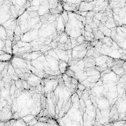
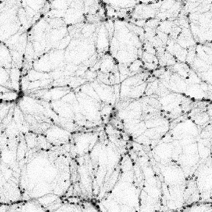
$\tau$CDM	$\Lambda$CDM

Figure 4: The left hand panel shows the locations of galaxies brighter than $M_{\mathrm{B}}-5\log h=-19.5$ in a $\tau$CDM model. The figure shows a slice of the dark matter simulation $85\times 85\times 4.7h^{-3}$ Mpc³ in size. The density of dark matter is indicated by the greyscale (with the densest regions being the darkest). Overlaid are the positions of the galaxies, indicated by open circles. The right hand panel shows the equivalent slice from a $\Lambda$CDM model (the GIF simulations all have the same phases, hence the similarity of the structure), the slice in this case being $141\times 141\times 8h^{-3}$ Mpc³ in size.

Figure 5: The left hand panel shows the two-point correlation function of galaxies brighter than $M_{\mathrm{B}}-5\log h=-19.5$ in a $\tau$CDM model as a solid line. The dashed lines to either side indicate the Poisson sampling errors. This is compared to the observed APM real-space correlation function (points with error bars) and to the mass correlation functions in the N-body simulations (dotted line). The right hand panel shows the equivalent plot for a $\Lambda$CDM model.

The results of the techniques described in the previous section are shown in Fig. 4 & 5. Fig. 4 shows slices through the GIF $\Lambda$CDM and $\tau$CDM dark matter simulations on which we have overlaid the positions of galaxies from our models. The galaxies can be seen to trace out structure in the dark matter and to avoid the underdense regions in the dark matter distribution. The galaxies clearly follow the large scale structure of the dark matter, but as we will show, they are biased tracers of the mass. The most obvious difference between the two diagrams is the smaller number of galaxies in the $\tau$CDM model. This is simply due to the smaller volume of the $\tau$CDM slice (approximately five times smaller than the $\Lambda$CDM slice), since the number of galaxies per unit volume is constrained to be very similar in each model by the requirement that they match the observed luminosity function.

Fig. 5 shows the two-point correlation functions of the model galaxies, and compares them to the observed APM correlation function (in real-space) and to the correlation function of the underlying dark matter. The two models show distinct differences in their behaviour. Most obviously, the $\Lambda$CDM model is very close to the APM data from $r\approx 0.3h^{-1}$ Mpc to $r\approx 10h^{-1}$ Mpc, whilst the $\tau$CDM model fails to achieve a large enough amplitude on scales $\geq 1.0h^{-1}$ Mpc and drops even further below the observed correlation function on smaller scales. The $\tau$CDM model shows a strong bias on large scales. The bias parameter, defined as the square root of the ratio of the galaxy and mass correlation functions, is approximately 1.4. The $\Lambda$CDM model, on the other hand, is essentially unbiased on large scales. Both models show an anti-bias on smaller scales. It is interesting to note that the galaxy correlation functions do not display the same features as the dark matter. For example the shoulder in the $\Lambda$CDM dark matter correlation function at 3 $h^{-1}$ Mpc is not present in the galaxy correlation function. Instead, the latter is remarkably close to a power-law form over about four orders of magnitude in amplitude.

3.2 Systematic effects

In this section we consider two systematic effects which may affect the clustering properties of galaxies in our models: dynamical friction in groups and clusters and our procedure for constructing merger trees for the dark matter halos. We show that neither of these significantly affects the two-point correlation function.

3.2.1 Dynamical friction

Our models do not accurately account for the effects of dynamical friction on the spatial position of satellite galaxies in halos. The simulations lack the resolution to follow this process directly. We can, however, correctly model the two extremes of this effect. If the dynamical friction timescale is much longer than the age of the halo, then the galaxy orbit is close to its original orbit, and so our placement scheme, consisting of identifying galaxies with randomly chosen halo particles, is correct on average. Conversely, if the dynamical friction timescale were much shorter than the halo lifetime, the satellite galaxy would have sunk to the bottom of the halo potential well and merged with the central galaxy. This effect is included in the semi-analytic model. Therefore, it is only in the intermediate range where the dynamical friction timescale is of the same order as the halo lifetime that our models do not accurately reproduce the galaxy positions within clusters.

To estimate the effect of dynamical friction on the correlation function we have tried perturbing the galaxy positions using the following simple model. From the calculation of the dynamical friction timescale in an isothermal halo given by Lacey & Cole (1993) (their equation B4), it can be seen that the orbital radius of a galaxy in a circular orbit, $r$, decays with time as

$$r=r_{\mathrm{i}}\sqrt{{t_{\mathrm{df}}-t\over t_{\mathrm{df}}}},$$ (1)

where $r_{\mathrm{i}}$ is the initial orbital radius of the galaxy when the halo forms, at $t=0$, and $t_{\mathrm{df}}$ is the dynamical friction timescale of the galaxy, given by Lacey & Cole (1993). Here, to mimic this behaviour, each satellite galaxy is first assigned a position in the halo tracing the dark matter as before and then its distance from the halo centre is reduced by a factor $r/r_{\mathrm{i}}$.

Fig. 6 shows the correlation function in our $\Lambda$CDM reference model with and without this dynamical friction effect included. Dynamical friction causes only a slight increase in the clustering amplitude on small scales, $<0.5h^{-1}$ Mpc, (since galaxies are drawn closer together inside halos). However the effect is small and can be safely neglected.

Figure 6: The correlation function in our $\Lambda$CDM reference model, with and without the effects of dynamical friction on satellite galaxy positions. The thin solid line shows the standard model (the dashed lines indicating the Poisson errors), whilst the thick lines show the same model with an estimate of dynamical friction effects included.

3.2.2 Merger tree construction

Figure 7: A comparison of correlation functions for galaxies brighter than $M_{\mathrm{B}}-5\log h=-19.5$ in our $\Lambda$CDM reference model with the results of a model with an artificial mass resolution designed to mimic the models of Kauffmann et al. (1999a). The low resolution model is shown as a thick solid line whilst our reference model is shown by thin solid lines. The dashed lines indicate the Poisson sampling errors.

As noted in §1, one difference between this work and that of Kauffmann et al. (1999a) is that they extract merger trees for dark matter halos directly from the N-body simulation, whereas we extract the final mass of the halo and generate the merger tree using the extended Press-Schechter Monte-Carlo formalism. There are advantages to both techniques. Extracting the halo trees from the simulation circumvents any possible discrepancy between the extended Press-Schechter predictions and the merging histories in the N-body simulation, although it has been shown that the two are statistically equivalent (see for example Lacey & Cole 1994; Lemson & Kauffmann 1999; Somerville et al. 1998). In particular, Lemson & Kauffmann (1997) have studied the statistical properties of halo formation histories in N-body simulations and find no detectable dependence of formation history on environment, as expected in the Press-Schechter theory. Thus, the fact that we construct merger trees similarly for halos in high and low-density regions should make little or no difference to our results. Furthermore, since here we are only interested in the statistical properties of the galaxy population, our approach is justified.

One drawback of the direct extraction technique is that the merging trees become limited by the resolution of the simulation. Like us, Kauffmann et al. identified halos containing at least 10 particles. Since this mass resolution limit applies at all times in the simulation, such a halo cannot have been formed by merging, as it might have done in a higher resolution simulation. Furthermore, even large mass halos might have significantly modified merging histories due to this artificial resolution limit. The analytic merging trees that we generate do not suffer from this problem. The effective mass and time resolutions can be made as small as desired, until convergence is reached. We demonstrate the effects of the resolution limit by considering a $\Lambda$CDM model in which we artificially impose an effective mass resolution equivalent to that in the Kauffmann et al. models. Fig. 7 shows that the differences between the models with and without the artificial mass resolution limit are, in general insignificant, although there is a region (approximately from separations of 0.4 to 1.5 $h^{-1}$ Mpc) where the disagreement between the two is significant.

Finally, it should be noted that since we extract the final masses of halos from the N-body simulation, our models do not suffer from the well-documented (but small) differences between the Press-Schechter and N-body mass functions at low mass (e.g. below $\sim 10^{14}h^{-1}M_{\odot}$), discussed by Efstathiou, Frenk, White & Davis (1988), Lacey & Cole (1994) and Somerville et al. (1998).

4 The nature of bias

Figure 8: The B-band mass-to-light ratio of halos in our models. The dotted line corresponds to $\tau$CDM and the solid line to $\Lambda$CDM. Lines show the median mass-to-light ratio, whilst the error bars indicate the 10 and 90 percentiles of the distribution. For reference, the mean mass-to-light ratio in the simulation as a whole is about 1440 and 470 $hM_{\odot}/L_{\odot}$ in the $\tau$CDM and $\Lambda$CDM cosmologies respectively, with an uncertainty of about 20% due to unresolved galaxies.

In the models explored here, galaxies do not trace the mass exactly because galaxy formation proceeds with an efficiency which depends on halo mass. In the lowest mass halos, feedback from supernovae prevents efficient galaxy formation, whilst in the high mass halos, gas is unable to cool efficiently by the present day thereby inhibiting galaxy formation. These effects can be seen in the mass-to-light ratios (in the B-band) of halos in our reference models plotted in Fig. 8. The mass-to-light ratio is strongly dependent on halo mass. Initially, it decreases as halo mass increases, before turning upwards and levelling off at close to the universal value for the highest mass halos in the simulations. The minimum, at around $10^{12}h^{-1}M_{\odot}$, marks a preferred mass scale at which the efficiency of galaxy formation is greatest. The mass-to-light ratio varies by more than a factor of 3 over the range of masses plotted here. As a result of this varying mass-to-light ratio we expect a complex, scale-dependent bias to arise and this is, in fact, seen in our two reference models. The clustering of galaxies is controlled by the intrinsic bias of their host halos, the non-linear dynamics of the dark matter and the processes of galaxy formation.

Figure 9: The mean number of galaxies, brighter than $M_{\mathrm{B}}-5\log h=-19.5$ per halo as a function of halo mass. The plots are for the $\tau$CDM (left hand panel) and the $\Lambda$CDM (right hand panel) models. Note that unoccupied halos are included when computing the mean. The thick solid line shows the mean number, $\bar{N}$, of galaxies per halo. The remaining lines indicate the mean number of galaxy pairs per halo as defined by Equation 3, for three different probability distributions, $P(N;M)$: “true” (thin solid line); “average” (dotted line) and “Poisson” (dashed line). Note the different scales in the two plots.

Fig. 9 shows the mean number of galaxies per halo as a function of halo mass in our two models. (For future reference we also plot the mean number of pairs of galaxies per halo as defined by Equation 3 below.) Below the $10^{12.5}h^{-1}M_{\odot}$ and $10^{13}h^{-1}M_{\odot}$ bins in the $\tau$CDM and $\Lambda$CDM models respectively, halos always contain zero or one galaxy (i.e. the number of pairs is zero). This is simply because there is not enough cold gas in the halo to form two or more galaxies of the required luminosity by the present day. At higher halo masses there is a trend of increasing number of galaxies per halo. The average occupation increases less rapidly than the halo mass, indicating once again that the halo mass-to-light ratio increases with increasing mass.

Galaxies brighter than some given absolute magnitude only form in halos above a certain mass, $M_{\mathrm{h}}$. On scales much larger than the radii of these halos, the correlation function of these galaxies will be proportional to that of the dark matter, with some constant, asymptotic, large-scale bias, as has been shown by Mo & White (1996). Behaviour of this type is seen in both of our reference models. This large scale bias can be estimated by averaging the Mo & White analytic bias for all halos of mass greater than $M_{\mathrm{h}}$, weighting by the abundance of those halos and by the number of galaxies residing (on average) within them (see Baugh et al. 1999).

On smaller scales the situation is more complex. The Mo & White calculations break down on scales comparable to the pre-collapse (Lagrangian) radius of the host halos. If halos of mass $M$ have a Lagrangian radius $R$, then we expect a reduction of the correlation of these halos on scales $\leq R$, since these objects must have formed from spatially exclusive regions of the universe. Halos may have moved somewhat after their formation and so will not be completely exclusive below this scale. However, they must be completely exclusive below their post-collapse (virial) radius ($R_{\mathbf{vir}}$), since no two halos can occupy the same region of space. Galaxies, however, resolve the internal structure of the halos and so we should not necessarily expect the same degree of anti-bias on sub-$R_{\mathrm{v}ir}$ scales in the galaxy distribution although these exclusion effects may still be apparent to some extent. Instead, the correlation function will begin to reflect the distribution of dark matter within the halos since, in our models, galaxies always trace the halo dark matter.

However, this is still not the whole picture. If $N(M)$ is the average number of galaxies per halo of mass $M$, then we can define a mass $M^{\prime}>M_{\mathrm{h}}$, where $N(M^{\prime})=1$ (here $M_{\rm h}$ is the minimum mass of a halo that can host a galaxy brighter than $M_{\rm B}-5\log h=-19.5$). We find $M^{\prime}=10^{13}$ and $10^{12}h^{-1}M_{\odot}$ for the $\tau$CDM and $\Lambda$CDM models respectively. In halos less massive than $M^{\prime}$, we typically find at most a single galaxy and so the distribution of dark matter within these halos is not resolved. Instead, our galaxy catalogue contains information only about the position of the halo centre. In general, the clustering will depend upon $P(N;M)$, the probability of finding $N$ galaxies in a halo of mass $M$. In particular, the small-scale clustering will depend upon the mean number of pairs per halo, which is itself determined by the form of the $P(N;M)$ distribution. Since the correlation function is a pair weighted statistic it gives extra weight to distributions with a tail to high $N$.

Figure 10: Correlation functions constructed from different samples of dark matter particles compared to the observed and model galaxy correlation functions in the $\tau$CDM reference model (left-hand panel). The various curves, labelled in the legend, are described in detail in the text. The right hand panel shows the same plots for the $\Lambda$CDM reference model.

The correlation function of galaxies is thus the result of a complex interplay of several effects: (i) asymptotic constant bias on large scales; (ii) spatial exclusion of halos; (iii) the number of galaxies per halo which controls whether the internal structure of the halos is resolved or not and (iv) the form of the $P(N;M)$ distribution (as this determines the mean number of pairs of galaxies per halo), which we discuss below. It is difficult, therefore, to construct an empirical model that reproduces the results of our full semi-analytic plus N-body models. It is, however, instructive to plot several correlation functions which act as bounds on the true galaxy correlation function.

Fig. 10 shows the correlation functions of galaxies in our model (thin solid line), dark matter in the simulation (dotted line), and observed galaxies in the APM survey, as measured by Baugh (1996) (squares with error bars). The short-dashed line is computed from all dark matter particles that are part of halos of mass greater than $M^{\prime}$ (i.e. halos sufficiently massive to contain galaxies at least some times). This curve is highly biased with respect to the full dark matter distribution, a fact that is not surprising given that it excludes the least clustered mass. We would expect the galaxy correlation function to be similar to this if the number of galaxies per halo were drawn from a Poisson distribution with mean proportional to the halo mass, that is, if the mass-to-light ratio were independent of halo mass. Evidently this is not the case. (The asymptotic bias of this correlation function is greater than that of the model galaxies (thin solid line), as weighting by halo mass gives more weight to the highly biased, most massive halos than does weighting by galaxy number.) The heavy solid line is the correlation function of halo centres, with each centre weighted by the model $P(N;M)$ distribution. The spatial exclusion of halos is evident, causing this curve to drop below that of the galaxies and finally to plummet to $\xi(r)=-1$ at a scale comparable to twice the virial radius of the smallest occupied halos.

The dot-dash line shows the correlation function found by placing in each halo the average number of galaxies per halo of each mass $\left[\sum_{N=1}^{\infty}NP(N;M)\right]$, using our usual placement scheme (i.e. the first galaxy is placed at the halo centre and the others are attached to random particles in the halo). We refer to this as the “average” model. Obviously, we cannot place the average number per halo if this is not an integer. In this case, we place a number of galaxies equal to either the integer immediately below or immediately above the actual mean with the relative frequencies needed to give the required mean, which results in a small scatter in the occupation. Finally, the long-dashed line shows the correlation function obtained when the number of galaxies in a halo is drawn from a Poisson distribution with the same mean as the model distribution (the “Poisson” model).

The differences between the correlation functions of the full semi-analytic model and models in which halos are occupied according to a Poisson distribution or simply with the average galaxy number (thin solid line, long-dashed line and dot-dash line respectively) must be due entirely to the form of $P(N;M)$ (i.e. the frequency with which a halo of a given mass is occupied by $N$ galaxies), since all these models are, by construction, identical in all other respects, including the mean halo occupation number. Fig. 11 illustrates the difference between the actual distribution of galaxies in all halos resolved in the simulations,

$$P(N)=\int^{\infty}_{M_{\rm min}}P(N;M)n(M)dM\left/\int^{\infty}_{M_{\rm min}}n(M)dM,\right.$$ (2)

and the “Poisson” and “average” models. Here $M_{\rm min}$ is the mass of the smallest halo that can be resolved in the simulation. The values of $P(N)$ in this plot are multiplied by $N(N-1)$ so that the area under the histogram gives the mean number of pairs per halo. The number of galaxies present in a halo is related to the structure of the merger tree for that halo. Although the merger tree is generated by a Monte-Carlo method, this does not produce a Poisson distribution of progenitor halos. Furthermore, whilst the Poisson distribution always possesses a tail to arbitrarily high numbers, the real distribution cannot as there is only enough cold gas in any one halo to make a limited number of bright galaxies.

Figure 11: The probability, $P(N)$, of occupation by $N$ galaxies (multiplied by $N(N-1)$ for clarity) for halos in the $\tau$CDM model (left hand panel) and $\Lambda$CDM model (right hand panel). All halos resolved in the simulations are considered. The solid line shows the distribution from the actual model, the dotted line shows the “Poisson” model distribution and the dashed line shows the “average” model distribution. Note that the $N=0$ and $N=1$ bins are always zero because we choose to weight $P(N)$ by $N(N-1)$.

Table 2 gives the mean number of pairs found within a single halo in the two reference models for all halos resolved in the simulation. This is given by

$$N_{\mathrm{P}}=\sum_{i=0}^{\infty}i(i-1){\int^{\infty}_{M_{\rm min}}P(i;M)n(M)dM\over\int^{\infty}_{M_{\rm min}}n(M)dM},$$ (3)

where $P(i;M)$ is the distribution of occupancies (normalised such that $\sum_{i=0}^{\infty}P(i;M)=1$) for halos of mass $M$ and $n(M)$ is the abundance of halos of mass $M$. The number of pairs in the “true”, “average” and “Poisson” distributions is shown in Figure 9. Note that if we consider two such halos separated by some distance $\sim r$ then the mean number of pairs at separation $\sim r$ is

$$\sum_{i=0}^{\infty}\sum_{j=0}^{\infty}ijP(i;M)P(j;M)=\bar{i}^{2}$$ (4)

and $\bar{i}$ is constrained to be equal in all three distributions.

Table 2: The mean number of pairs per halo, $N_{\mathrm{P}}$, calculated for three different distributions of halo occupancy, all with the same mean. “Average” has the same number of galaxies in all halos in a given mass range (or as close to this distribution as possible if the mean is not an integer), “true” has the distribution found in our reference models and “Poisson” has a Poisson occupation.

Model	average	true	Poisson
$\tau$CDM	0.0005	0.0010	0.0116
$\Lambda$CDM	0.0538	0.0678	0.1262

Thus, we can understand the difference in the clustering amplitudes of the three correlation functions at small scales (they all agree within the errors at large scales) simply on the basis of the form of their $P(N;M)$ function which determines the mean number of pairs per halo, $N_{\mathrm{P}}$. For distributions with the same mean, the one with the lowest number of pairs per halo, $N_{\mathrm{P}}$, will have the lowest clustering amplitude, whilst the one with the largest number of pairs will have the highest clustering amplitude. (In the case of the “average” and “true” distributions, the correlation functions are very similar on small scales as the contribution from pairs of galaxies within a single halo is small compared to that from pairs in distinct halos.) The consequence of this is that the amplitude of the small scale end of the observed correlation function tells us something interesting about $P(N;M)$, namely that it has fewer pairs than a Poisson distribution and is in reasonable agreement with the distribution predicted from our semi-analytic model. Thus, the behaviour of the small separation end of the correlation function is determined by the physics of galaxy formation. We have checked that our choice of placing central galaxies at the centre of mass of their halo does not affect these results. If instead each central galaxy is placed on a randomly chosen dark matter particle (i.e. if treated just like a satellite galaxy) the correlation function is unaltered within the error bars.

The $\tau$CDM reference model shows a break on sub-Mpc scales. As can be seen in Fig. 10 this coincides with the turnover in the correlation function of halo centres. This turnover is reflected in the galaxy correlation function because in this model there are too few bright galaxies in cluster halos to resolve adequately their internal structure. In the $\Lambda$CDM models, on the other hand, halos are adequately resolved and the galaxy correlation function remains almost a power-law, even though that of halo centres turns over. To remove this feature from the $\tau$CDM model would require more bright galaxies to form in cluster halos. However, this would have to be accomplished without significantly increasing the number of bright galaxies in lower mass halos since these would quickly come to dominate the asymptotic bias which would therefore become lower than its present value thus exacerbating the discrepancy between model and observations at large separations. We have been unable to find a model constrained to match the local luminosity function which succeeds in removing the sub-Mpc feature in our $\tau$CDM model whilst simultaneously producing the required asymptotic bias.

The reason for the differences between the two reference models is illustrated in Fig. 12, where we compare our models to an observational determination of the “luminosity function of all galactic systems.” This function, estimated by Moore, Frenk & White (1993), gives the abundance of halos as a function of the total amount of light they contain, regardless of how it is shared amongst individual galaxies. This quantity is difficult to determine observationally, since one must establish which galaxies are in the same dark matter halo. Moore, Frenk & White (1993) approached this problem by analysing the “CfA-1” galaxy redshift survey (?, ?) using a modified friends-of-friends group finding algorithm which was allowed to have different linking lengths in the radial and tangential directions to account for redshift-space distortions. These linking lengths were also allowed to vary with distance, to reflect the changing number density of galaxies in the survey. It is entirely possible, however, that in some instances this technique may have grouped together galaxies which actually reside in distinct dark matter halos. Finally, Moore, Frenk & White (1993) made a correction to the luminosity of each identified group to account for the light from unseen galaxies (i.e. those below the magnitude limit of the survey). This was done assuming a universal form for the galaxy luminosity function. Such a form may not, in fact, be applicable to the real Universe, and is not guaranteed to arise in our models.

Bearing these caveats in mind, we see in Fig. 12 that the $\Lambda$CDM reference model and the data are in excellent agreement except at the faint end where the discrepancy reflects the fact that the data come from the CfA-1 Survey which has a flatter luminosity function than the ESO Slice Project (ESP) luminosity function we used to constrain our semi-analytic model. By contrast, the $\tau$CDM model fails to match the luminosity function of all galactic systems, in spite of the fact that it agrees quite well with the bright end of the galaxy luminosity function (c.f. Fig. 1). This model does not make enough bright galaxies in high mass, highly clustered halos and it makes too many in low mass, weakly clustered halos. It is not surprising therefore that the $\tau$CDM galaxy correlation function falls below the observed data on all scales (c.f. Fig. 13). A similar conclusion applies to the standard $\Omega_{0}=1$ CDM model although in this case the disagreement with the observed correlation function on large scales is even worse than in the $\tau$CDM model. Matching the luminosity function of all galaxy galactic systems is, therefore, an important prerequisite for a model to match the two-point correlation function.

Figure 12: The luminosity function of all galactic systems. Results for our $\tau$CDM model are shown with the short-dashed line and for our $\Lambda$CDM model with the solid line. The symbols with error bars are the observational data from Moore, Frenk & White (1993). The horizontal lines indicate the abundance below which the probability of finding one or more such objects in the entire volume of the simulation is less than 10% in the $\tau$CDM (long dashed line) and $\Lambda$CDM (dotted line) models.

5 Testing the robustness of the predictions

The semi-analytic model of galaxy formation is specified by several parameters. These determine the cosmological model and control astrophysical processes such as star formation, supernovae feedback and galaxy merging. Whilst these parameters can be constrained by requiring the model to reproduce certain local observations (such as the B and K-band luminosity functions; see Cole et al. 1999), we wish to explore here what effect altering these parameters has on our estimate of the correlation function.

Thus, we alter the parameters of the reference model one at a time. We try to preserve as good a match as possible to the local B-band luminosity function by giving ourselves the freedom of adjusting the value of $\Upsilon$ so that the model B-band luminosity function has the correct amplitude at $L_{*}$. Since the reference models give a good match not only to the B-band luminosity function, but also to a variety of other observational data (such as the distribution of colours, sizes, star formation rates, etc.), the modified models will, in general, not be as good as the reference models. Furthermore, in some cases matching the $M_{\mathrm{B}}-5\log h=-19.6$ point of the ESP luminosity function requires $\Upsilon<1$ which is unphysical (as it implies negative mass in brown dwarfs). However, this is not a serious concern here since we are only interested in testing the robustness of clustering properties to changes in model parameters. We also consider a few models in which $\Upsilon$ is set so as to match the zero-point of the I-band Tully-Fisher relation, rather than the amplitude of the luminosity function at $L_{*}$. These are closer to the models of Kauffmann et al. (1999a).

The semi-analytic model with the altered parameters is used to populate the N-body simulation with galaxies. We then measure the bias of galaxies brighter than $M_{\rm B}-5\log h=-19.5$ in each model.

5.1 Models constrained by the luminosity function

Both of our reference models which are constrained to match the $M_{\mathrm{B}}-5\log h=-19.6$ point of the ESP luminosity function (Zucca et al. 1997), also reproduce the observed exponential cut-off at the bright end of the local B and K-band luminosity functions (cf. Fig. 1). This fact turns out to be of importance when studying the clustering of these galaxies.

Table 3: Variant models in $\tau$CDM cosmologies. The first column gives the value of the parameter which is varied relative to the reference model. The remaining columns give the values of $\Upsilon$ used to match a point in the luminosity function for each model and the asymptotic bias of the galaxies estimated from the fitting formula of Jing (1998), $b_{\mathrm{a}nalytic}$, and from our models, $b_{\mathrm{m}odel}$.

Model	$\Upsilon$	$\mathbf{b_{\mathrm{analytic}}}$	${\mathbf{b}}_{\mathrm{model}}$
Reference	1.23	1.27	1.65 $\pm$ 0.37
$v_{\mathrm{hot}}=350$ km/s	1.06	1.27	1.62 $\pm$ 0.36
$v_{\mathrm{hot}}=200$ km/s	1.41	1.26	1.57 $\pm$ 0.29
$\alpha_{*}=-0.25$	1.20	1.27	1.62 $\pm$ 0.33
$\alpha_{*}=-1.50$	1.33	1.27	1.63 $\pm$ 0.40
$\epsilon_{*}=0.01^{{\dagger}}$	0.98	1.27	1.64 $\pm$ 0.28
$\epsilon_{*}=0.04$	1.52	1.29	1.72 $\pm$ 0.42
$f_{\mathrm{d}f}=0.5^{{\dagger}}$	1.17	1.27	1.67 $\pm$ 0.44
$f_{\mathrm{d}f}=0.03$	1.23	1.25	1.59 $\pm$ 0.35
IMF: Kennicutt (1993)	2.01	1.29	1.65 $\pm$ 0.38
$r_{\mathrm{core}}=0.2$	1.22	1.26	1.60 $\pm$ 0.39
$r_{\mathrm{core}}=0.02$	1.23	1.28	1.65 $\pm$ 0.36
$\Omega_{\mathrm{b}}=0.10$	1.82	1.28	1.59 $\pm$ 0.31
$\Omega_{\mathrm{b}}=0.05$	0.55	1.26	1.71 $\pm$ 0.36
$p=0.02$	1.20	1.29	1.69 $\pm$ 0.38
Recooling	1.68	1.28	1.64 $\pm$ 0.36
No dust	1.89	1.30	1.68 $\pm$ 0.36

^† The two models with the greatest deviation from the mean two-point correlation function.

Table 4: Variant models in $\Lambda$CDM cosmologies. The first column gives the value of the parameter which is varied relative to the reference model. The remaining columns give the values of $\Upsilon$ used to match a point in the luminosity function for each model and the asymptotic bias of the galaxies estimated from the fitting formula of Jing (1998), $b_{\mathrm{a}nalytic}$, and from our models, $b_{\mathrm{m}odel}$.

Model	$\Upsilon$	$\mathbf{b_{\mathrm{analytic}}}$	${\mathbf{b}}_{\mathrm{model}}$
Reference	1.63	1.07	1.01 $\pm$ 0.03
$v_{\mathrm{hot}}=200$ km/s	1.45	1.07	0.98 $\pm$ 0.01
$v_{\mathrm{hot}}=100$ km/s	1.53	1.06	0.97 $\pm$ 0.02
$\alpha_{*}=-0.25$	1.63	1.08	0.98 $\pm$ 0.01
$\alpha_{*}=-1.50$	1.58	1.06	0.97 $\pm$ 0.01
$\epsilon_{*}=6.67\times 10^{-3}$	1.33	1.06	0.98 $\pm$ 0.01
$\epsilon_{*}=0.02$	1.81	1.06	0.97 $\pm$ 0.01
$f_{\mathrm{d}f}=5.0^{{\dagger}}$	1.29	0.93	0.88 $\pm$ 0.02
$f_{\mathrm{d}f}=0.2^{{\dagger}}$	1.31	0.98	0.91 $\pm$ 0.01
IMF: Salpeter (1955)	0.90	1.01	1.00 $\pm$ 0.02
$r_{\mathrm{core}}=0.2$	1.63	1.07	0.98 $\pm$ 0.01
$r_{\mathrm{core}}=0.02$	1.63	1.07	0.99 $\pm$ 0.01
$\Omega_{\mathrm{b}}=0.04^{{\dagger}}$	2.04	1.13	1.02 $\pm$ 0.01
$\Omega_{\mathrm{b}}=0.01^{{\dagger}}$	0.70	0.96	0.95 $\pm$ 0.02
$p=0.04^{{\dagger}}$	1.04	1.11	1.01 $\pm$ 0.01
Recooling†	1.67	1.11	1.00 $\pm$ 0.02
No dust	2.31	1.04	0.95 $\pm$ 0.01

^† The six models with the greatest deviation from the mean two-point correlation function.

Figure 13: Correlation functions in the $\tau$CDM (left hand panel) and $\Lambda$CDM (right hand panel) cosmologies. All the models are constrained to match the abundance of $L_{*}$ galaxies in the ESP B-band luminosity function. In each plot the points with error bars show the observed APM real-space correlation function of Baugh (1996), whilst the dotted line shows the correlation function of the dark matter. The model galaxy correlation functions are shown as solid lines except in the case of models which deviate substantially from the average of all models which are shown as dashed lines.

Figure 14: B-band luminosity functions in the $\tau$CDM (left hand panel) and $\Lambda$CDM (right hand panel) models. All models are constrained to match the ESP luminosity function of Zucca et al. (1997) at $M_{\mathrm{B}}-5\log h=-19.56$. Symbols with error bars show a selection of observational determinations of the luminosity functions, from the sources indicated in the legend. The solid lines show results for our models, except that the outliers identified in Fig. 13 are shown as dashed lines. Each luminosity function is plotted only to the completeness limit of the simulations.

Figure 15: The average number of galaxies brighter than $M_{\mathrm{B}}-5\log h=-19.5$ per halo as a function of halo mass. The panels refer to the $\tau$CDM models (left) and the $\Lambda$CDM models (right). Note that unoccupied halos are counted. Dashed lines indicate the outlier models identified in Fig. 13. (Some of the lines lie on top of one another because the corresponding changes in model parameters do not alter the number of galaxies per halo.)

Tables 3 & 4 list the variant models that we have studied in the $\tau$CDM and $\Lambda$CDM cosmologies respectively. The first column of each table lists those parameters that have changed from the reference model (which is listed in the first row of the tables). “Recooling” models allow enriched gas reheated by supernovae to recool within a dark matter halo. All but one model use the “No recooling” algorithm in which this gas is not allowed to recool until its halo doubles in mass. In the “No dust” models we do not account for extinction by internal dust (see Cole et al 1999). Also listed in the tables is the value of $\Upsilon$ for each model and the average analytic asymptotic bias of the galaxies calculated as follows:

$$b_{\mathrm{a}nalytic}=\sum^{N}_{i=1}b(M_{i})/N\equiv{\int_{0}^{\infty}b(M)\bar{N}(M)n(M){\mathrm{d}}M\over\int_{0}^{\infty}\bar{N}(M)n(M){\mathrm{d}}M},$$ (5)

where $N$ is the number of galaxies in the catalogue, $M_{i}$ is the mass of the halo hosting the $i^{\mathrm{t}h}$ galaxy, $\bar{N}(M)$ is the mean number of galaxies per halo of mass $M$, and $n(M)$ is the dark matter halo mass function in the simulation. The function $b(M)$ is the asymptotic bias of halos of mass $M$ which we estimate using Jing’s (1998) formula obtained from fitting the results of N-body simulations. This formula tends to the analytic result of Mo & White (1996) for masses much greater than $M_{*}$. The final column gives the asymptotic bias estimated directly from our models, on scales where $\xi_{\mathrm{m}atter}(r)<1$ ($\approx 2.5$ and $5.0h^{-1}$ Mpc in the $\tau$CDM and $\Lambda$CDM cosmologies respectively), as described by Jing (1998). Note that the analytic biases are consistently lower than those measured in our $\tau$CDM models. The halos in the $\tau$CDM GIF simulation show a similar disagreement with the fitting formula of Jing (1998) which was tested on SCDM, OCDM and $\Lambda$CDM cosmologies only. The models marked by a dagger are those showing large deviations from the mean clustering amplitude of all models (six and two such models are identified in the $\Lambda$CDM and $\tau$CDM cosmologies respectively).

In the remainder of this section we show the correlation functions obtained from these variant models and discuss how the form of the correlation function is related to other properties of the galaxy population. The correlation functions are displayed in Fig. 13. All cases show antibias on small scales and a constant bias on large scales. Most of the models in both cosmologies have similar correlation functions but the scatter is somewhat greater in the $\tau$CDM case than in the $\Lambda$CDM case. The models that deviate most from the average are shown as dashed lines in Fig. 13 and also in all other plots in this section. In the $\Lambda$CDM cosmology, where the reference model is well fit by a power-law correlation function, the deviant models have slopes which are somewhat different from the other models.

The luminosity functions in most of the $\Lambda$CDM models, plotted as solid lines, in Fig. 14, are quite similar. (They are all forced to go through the same point at $M_{\mathrm{B}}-5\log h=-19.6$.) The ones that deviate the most are those plotted as dashed lines, that is, those that were identified in Fig. 13 as giving the most discrepant correlation functions. Thus, we see that the main factor that determines the sensitivity of the correlation function to model parameters is the ability of the model to reproduce the exponential cut-off observed in the luminosity function. Models that achieve this all give similar galaxy correlation functions. A similar conclusion applies in the $\tau$CDM case, although here the distinction is less clearcut due to our noisy estimates of the correlation function on small scales.

We have also considered two models that have different dark matter power spectra. These make use of the GIF SCDM and OCDM simulations (described in §2) and, apart from the values of the cosmological parameters, they have the same parameter values as our reference $\tau$CDM and $\Lambda$CDM models respectively. Whilst the OCDM model shows very little difference from the $\Lambda$CDM model, the SCDM model has a significantly different clustering amplitude than our reference $\tau$CDM model (approximately 40% lower on scales larger than 1 Mpc). Despite this its luminosity function is in fairly close agreement with that of the $\tau$CDM model at the bright end. This model therefore demonstrates that models with the same luminosity function only produce the same correlation function if they have the same underlying dark matter distribution.

As described in §3 the distribution of the number of galaxies per halo as a function of halo mass is very important in determining the behaviour of the correlation function. On small scales, the full distribution determines the amplitude and slope of the correlation function, whilst on large scales the number of galaxies per halo determines the asymptotic bias of the galaxy distribution by selecting the range of host halo masses that dominates the correlation function. Fig. 15 shows the number of galaxies per halo as a function of halo mass in our models. It is apparent, particularly for $\Lambda$CDM, that the models identified as outliers in the correlation function plot (Fig. 13) are also the ones that deviate the most from the reference models in these plots as well.

Figure 16: The B-band luminosity function (left) and galaxy correlation function (right) for two $\tau$CDM models constrained to match the I-band Tully-Fisher relation. The thin line in both panels corresponds to our reference model (but with the value of $\Upsilon$ required by the Tully-Fisher relation) and the thick lines corresponds to a model with very weak feedback. The luminosity function is shown only to the completeness limit of this model. In the right hand panel the symbols with error bars show Baugh’s (1996) APM correlation function, the dashed lines the Poissonian errors on the correlation functions, and the the dotted line the dark matter correlation function.

5.2 Models constrained by the Tully-Fisher relation

We have shown that matching the local galaxy luminosity function – our preferred method for constraining the parameters of our semi-analytic model – leads to model predictions for galaxy clustering that are robust to reasonable changes in these parameters. Kauffmann et al. (1999a) adopted a different philosophy: they chose to constrain their models by matching the I-band Tully-Fisher relation, rather than the luminosity function. We explore the effect of this choice by constraining our own models in a similar way. Specifically, we require the median magnitude of central spiral galaxies with halo circular velocities in the range 215.0 to 225.0 km s^-1 to be $M_{\mathrm{I}}-5\log h=-22.0$ (where $M_{\rm I}$ is the dust-extincted I-band magnitude of each galaxy corrected to the face-on value). This can be achieved by a suitable choice of the luminosity normalisation parameter, $\Upsilon$, and leads to a model Tully-Fisher relation that agrees well with data from Mathewson, Ford & Buchhorn (1992).

Since our original $\Lambda$CDM models (that is, the reference model and its variants) already agreed quite well with the Tully-Fisher relation, (see Fig. 2), this different choice of constraint has only a minor effect on the correlation function. The only noticeable change is an increase in the scatter of the asymptotic bias in the variant models. In the $\tau$CDM models, on the other hand, the new constraint has an important effect because the original models that agreed well with the luminosity function, missed the Tully-Fisher relation by about 1 magnitude. Forcing a fit to the Tully-Fisher relation destroys the good agreement of the reference model with the luminosity function, as may be seen in Fig. 16. This figure also shows a $\tau$CDM model in which we have attempted to obtain a better luminosity function by dramatically reducing the amount of supernovae feedback into the interstellar gas.

Fig. 16 shows that our two $\tau$CDM models that match the Tully-Fisher relation have different correlation functions. In other words, this exercise demonstrates that when models are constrained in this way, the resulting correlation functions are rather sensitive to the choice of model parameters. This explains why Kauffmann et al. (1999a) concluded that their clustering predictions depended strongly on the way they parametrised star formation, feedback and the fate of reheated gas in their model. By contrast, we have found that our predictions for the correlation function are robust to changes in model parameters, so long as the models match the bright end of the galaxy luminosity function.

6 Discussion and Conclusions

In this study, we have considered some of the physical and statistical processes that determine the distribution of galaxies and its relation to the distribution of mass in cold dark matter universes. The approach that we have adopted exploits two of the most successful techniques currently used in theoretical cosmological studies: N-body simulations to follow the clustering evolution of dark matter and semi-analytic modelling to follow the physics of galaxy formation. Our main conclusion is that the efficiency of galaxy formation depends in a non-trivial fashion on the mass of the host dark matter halo and, as a result, galaxies, in general, have a markedly different distribution from the mass. This result had been anticipated in early cosmological studies (eg. Frenk, White & Davis 1983, Davis et al. 1985, Bardeen et al. 1986), but it is only with the development of techniques such as semi-analytic modelling that realistic calculations have become possible.

The statistics of the spatial distribution of galaxies reflect the interplay between processes that determine the location where dark matter halos form and the manner in which halos are “lit up” by galaxy formation. If the resulting mass-to-light ratio of halos were independent of halo mass, then the distribution of galaxies would be related in a simple manner to the distribution of dark matter in halos. In current theories of galaxy formation, however, the mass-to-light ratio has a complicated dependence on halo mass. On small mass scales, galaxy formation is inhibited by the reheating of cooled gas through feedback processes, whereas in large mass halos it is inhibited by the long cooling times of hot gas. As a result, the mass-to-light ratio has a deep minimum at the halo mass, $\sim 10^{12}M_{\odot}$, associated with $L_{*}$ galaxies, where galaxy formation is most efficient. Although our calculations assume a specific model of galaxy formation, the dependence of mass-to-light ratio on halo mass displayed in Fig. 8 is likely to be generic to this type of cosmological model. The consequence of such a complex behaviour is a scale dependent bias in the distribution of galaxies relative to the distribution of mass.

On scales larger than the typical size of the halos that harbour bright galaxies, the bias in the galaxy distribution is related in a simple way to the bias in the distribution of massive halos. In our $\Omega_{0}=1$ $\tau$CDM model, galaxies end up positively biased on large scales, but in our flat, $\Omega_{0}=0.3$ $\Lambda$CDM model, they end up essentially unbiased. On small scales, the situation is more complicated and the correlation function depends on effects such as the spatial exclusion of dark matter halos, dynamical friction, and the number of galaxies per halo. In particular, our simulations show how the statistics of the halo occupation probability influence the amplitude of the galaxy correlation function on sub-megaparsec scales. In our models, the occupation of halos by galaxies is not a Poisson process. Since the amount of gas available for star formation is limited, the mean number of pairs per halo is less than that of a Poisson distribution with the same mean. This property plays an important role in determining the amplitude of small scale correlations.

Remarkably, the correlation function of galaxies in our $\Lambda$CDM model closely approximates a power-law over nearly four orders of magnitude in amplitude. This is in spite of the fact that the correlation function of the underlying mass distribution is not a power-law, but has two inflection points in the relevant range of scales. Somehow, the various effects just discussed conspire to compensate for these features in the mass distribution. In particular, on scales smaller than $\sim 3h^{-1}$ Mpc, the galaxy distribution in the $\Lambda$CDM model is antibiased relative to the mass distribution. The apparently scale-free nature of the galaxy correlation function in this model seems to be largely a coincidence (although whether this is also true of the real universe remains to be seen). Our $\tau$CDM model which has similar physics although a different initial mass fluctuation spectrum, does not end up with a power-law galaxy correlation function.

Colín et al. (1999) have carried out a very high resolution N-body simulations (of a $\Lambda$CDM cosmological model similar to ours) which resolves some substructure within dark matter halos. The correlation function of these sub-halos is remarkably similar to the correlation function of the galaxies in our $\Lambda$CDM reference model. In a sense, the merger trees of our semi-analytic models keep track of sub-halos within dark matter halos since they follow the galaxies that form within them. (Unlike the simulations, however, the semi-analytic model does not follow the spatial distribution of sub-halos.) Colín et al. select sub-halos by circular velocity, whereas we select galaxies by luminosity. Since, in our models, the luminosity of a galaxy is correlated with the circular velocity of the halo in which it formed, there is some correspondence between the type of objects studied by Colín et al. and us. However, the connection could be complicated by effects such as tidal disruption or stripping of halos within halos but which are not included in our model. Nevertheless, the abundance of sub-halos considered by Colín et al is similar to the abundance of galaxies in our $\Lambda$CDM model and this might account for the similarity between the two correlation functions.

Another noteworthy outcome of our simulations is the close match of the galaxy correlation function in our $\Lambda$CDM model to the observed galaxy correlation function, itself also a power-law over a large range of scales (Groth & Peebles 1977; Baugh 1996). This match is particularly interesting because the parameters that specify our semi-analytic galaxy formation model were fixed beforehand by considerations that are completely separate from galaxy clustering (see Cole et al. 1999). Our procedure for fixing these parameters places special emphasis on obtaining a good match to the observed galaxy luminosity function (c.f. Fig. 1), but makes no reference whatsoever to the spatial distribution of the galaxies.

To summarize, the combination of high resolution N-body simulations with semi-analytic modelling of galaxy formation provides a useful means for understanding how the process of galaxy formation interacts with the process of cosmological gravitational evolution to determine the clustering pattern of galaxies. In general, we expect galaxies to be clustered somewhat differently from the dark matter, and the relation between the two can be quite complex. A flat CDM model with $\Omega_{0}=0.3$ gives an acceptable match to the observed galaxy correlation function over about four orders of magnitude in amplitude (as does an open model with the same value of $\Omega_{0}$.) The $\Lambda$CDM model is also in reasonable agreement with a number of other known properties of the galaxy distribution.

References

- [1] [] Adelberger K. L., Steidel C. C., Giavalisco M., Pettini M., Kellogg M., 1998, ApJ, 505, 18
- [2] [] Bagla J. S., 1998, MNRAS, 299, 417
- [3] [] Bardeen J.M., Bond J.R., Kaiser N., Szalay A.S., 1986, ApJ, 304, 15
- [4] [] Baugh C. M., 1996, MNRAS, 280, 267
- [5] [] Baugh C. M., Cole S, Frenk C. S., Lacey C. G., 1998, ApJ, 498, 504
- [6] [] Baugh C. M., Benson A. J., Cole S., Frenk C. S., Lacey C. G., 1999, MNRAS, 305, L21
- [7] [] Blanton M., Cen R., Ostriker J. P., Strauss M. A., Tegmark M., 1999, astro-ph/9903165
- [8] [] Bond J. R., Kaiser N., Cole S., Efstathiou G., 1991, ApJ, 379, 440
- [9] [] Bower R.G., 1991, MNRAS, 248, 332
- [10] [] Cole S., Lacey C. G., Baugh C. M., Frenk C. S., 1999, MNRAS submitted
- [11] [] Colín P., Klypin A., Kravtsov A., Khokhlov A., 1999, ApJ, 523, 32
- [12] [] Colless M., 1996, in proceedings of the Heron Island Conference, http://msowww.anu.edu.au/ heron/Colless/colless.html
- [13] [] Davis M., Huchra J., Latham D. W., Tonry J., 1982, ApJ, 253, 423
- [14] [] Davis M., Peebles P. J. E., 1983, ApJ, 267, 465
- [15] [] Davis M., Efstathiou G., Frenk C. S., White S. D. M., 1985, ApJ, 292, 371
- [16] [] Diaferio A., Kauffmann G., Colberg J. M., White S. D. M., 1999, MNRAS, 307, 537
- [17] [] Efstathiou G., Frenk C.S., White S.D.M., Davis M., 1988, MNRAS, 235, 715
- [18] [] Efstathiou G., Bond J. R., White S.D.M., 1992, MNRAS, 258, 1
- [19] [] Evrard A. E., Summers F. J., Davis M., 1994, ApJ, 422, 11
- [20] [] Ferrara A., Bianchi S., Cimatti A., Giovanardi C., 1999, ApJS, 123, 437
- [21] [] Frenk C. S., White S. D. M., Davis M., 1983, ApJ, 271, 417
- [22] [] Gardner J. P., Sharples R. M., Frenk C. S., Carrasco B. E., 1997, ApJ, 480, L99
- [23] [] Glazebrook K., Ellis R., Colless M., Broadhurst T., Allington-Smith J., Tanvir N., 1995, MNRAS, 273, 157
- [24] [] Governato F., Baugh C. M., Frenk C. S., Cole S., Lacey C. G., Quinn T., Stadel J., 1998, Nat, 392,359
- [25] [] Gross M. A. K., Somerville R. S., Primack J. R., Holtzman J., Klypin A., 1998, MNRAS, 301, 81
- [26] [] Gunn J. E., Weinberg D. H., 1995, Wide-Field Spectroscopy and the Distant Universe, proceedings of the 35th Herstmonceux workshop, Cambridge University Press, Cambridge
- [27] [] Groth E. J., Peebles P. J. E., 1977, ApJ, 217, 38 ella M., Scaramella R., Stirpe G. M., Vettolani G., 1999, astro-ph/9901378
- [28] [] Hamilton A. J. S., Kumar P., Lu E., Matthews A., 1991, ApJ, 374, L1
- [29] [] Huchra J. P., Davis M., Latham D. W., Tonry J., 1983, ApJS, 53, 89
- [30] [] Jenkins A., Frenk C. S., Pearce F. R., Thomas P. A., Colberg J. M., White S. D. M., Couchman H. M. P., Peacock J. P., Efstathiou G., Nelson A. H., (The Virgo Consortium), 1998, ApJ, 499, 20
- [31] [] Jing Y. P., 1998, ApJ, 503, L9
- [32] [] Katz N., Hernquist L., Weinberg D. H., 1992, ApJ, 399, 109
- [33] [] Kauffmann G., Nusser A., Steinmetz M., 1997, MNRAS, 286, 795
- [34] [] Kauffmann G., Colberg J. M., Diaferio A., White S. D. M., 1999a, MNRAS, 303, 188
- [35] [] Kauffmann G., Colberg J. M., Diaferio A., White S. D. M., 1999b, MNRAS, 307, 529
- [36] [] Kennicutt, R. 1983, ApJ, 272, 54
- [37] [] Lacey, C.G., Cole, S., 1993, MNRAS, 262, 627
- [38] [] Lacey C. G., Cole S., 1994, MNRAS, 271, 676
- [39] [] Lemson G., Kauffmann G., 1999, MNRAS, 302, 111
- [40] [] Loveday J., Peterson B. A., Efstathiou G., Maddox S. J., 1992, ApJ, 390, 338
- [41] [] Mathewson D. S., Ford V. L., Buchhorn M., 1992, ApJS, 81, 413
- [42] [] Mo H. J., White S. D. M., 1996, MNRAS, 282, 347
- [43] [] Mobasher B., Sharples R. M., Ellis R. S., 1993, MNRAS, 263, 560
- [44] [] Moore B., Frenk C.S., White S.D.M., 1993, MNRAS, 261, 827
- [45] [] Navarro J. F., Frenk C. S., White S. D. M., 1996, ApJ, 462, 563
- [46] [] Peacock J. A., Dodds S. J., 1996, MNRAS, 280, L19
- [47] [] Pearce F. R., Jenkins A., Frenk C. S., Colberg J. M., White S. D. M., Thomas P. A., Couchman H. M. P., Peacock J. A., Efstathiou G. (The VIRGO Consortium), ApJ, 512, L99
- [48] [] Press W. H., Schechter P., 1974, ApJ, 187, 425
- [49] [] Ratcliffe A., Shanks T., Parker Q. A., Fong R., 1998, MNRAS, 296, 173
- [50] [] Roukema B. F., Peterson B. A., Quinn P. J., Rocca-Volmerange B., 1997, MNRAS, 292, 835
- [51] [] Salpeter, E.E., 1955, ApJ, 121, 61
- [52] [] Somerville R.S., Lemson G., Kolatt T.S., Dekel A., 1998, astro-ph/9807277 (submitted to MNRAS)
- [53] [] Tegmark M., Peebles P. J. E., 1998, ApJ, 500, 79
- [54] [] Owen J. M., Weinberg D. H., Evrard A. E., Hernquist L., Katz N., 1998, ApJ, 503, 160
- [55] [] White S. D. M., Frenk C. S., 1991, ApJ, 379, 52
- [56] [] Zucca E., Zamorani G., Vettolani G., Cappi A., Merighi R., Mignoli M., Stirpe G. M., MacGillivray H., Collins C., Balkowski C., Cayatte V., Maurogordato S., Proust D., Chincarini G., Guzzo L., Maccagni D., Scaramella R., Blanchard A., Ramella M., 1997, A&A, 326, 477