Identification of Moving Groups and Member Selection using Hipparcos Data

Abstract

A new method to identify coherent structures in velocity space — moving groups — in astrometric catalogues is presented: the Spaghetti method. It relies on positions, parallaxes, and proper motions and is ideally suited to search for moving groups in the Hipparcos Catalogue. No radial velocity information is required.

The method has been tested extensively on synthetic data, and applied to the Hipparcos measurements for the Hyades and IC2602 open clusters. The resulting lists of members agree very well with those of Perryman et al. for the Hyades and of Whiteoak and Braes for IC2602.

1 Introduction

The kinematical distribution of stars in the Solar neighborhood is far from smooth. In 1869 Proctor already discovered the existence of groups of stars in the same region of the sky that share kinematic properties. These groups are the result of the common motion of young stars produced by the localized nature of star formation in the Galaxy. Although most of these groups are confined in configuration space we define a moving group as a set of stars which occupy a small volume in velocity space. The distribution of these stars in configuration space does not enter in this definition. Among these groups are gravitationally bound open clusters (e.g., the Hyades [Perryman et al. 1998]), unbound OB associations (e.g., the Sco OB2 association [de Geus, de Zeeuw & Lub 1989]), and the so-called superclusters (e.g., Eggen 1991, Chereul, Crézé & Bienaymé 1998, 1999). Observational properties of such groups such as, the initial mass function (e.g., Claudius & Grosbøl 1980; Brown, de Geus & de Zeeuw 1994; Massey, Johnson & DeGioia-Eastwood 1995), the local star formation rate and efficiency (e.g., Williams & McKee 1997), and the fraction and characteristics of binary and multiple stars (e.g., Blaauw 1991; Brandner et al. 1996; Verschueren, David & Brown 1996), serve as important tests for current theories on star formation. These properties and the calibration of the distance scale and absolute magnitudes depend sensitively on membership. Therefore, it is crucial to have detailed knowledge of membership of moving groups, in particular open clusters and OB associations. As the velocity dispersions in moving groups are small, typically a few ${\rm km}~{}{\rm s}^{-1}$ or less (see e.g., Jones & Herbig 1979; Hartmann et al. 1986; Mathieu 1986; Tian et al. 1996), proper motions and radial velocities can be used to detect the common space motion and thus determine membership.

For the majority of the moving group candidate members, only proper motions or radial velocities are available. Several methods have been developed in this century to disentangle moving group stars from a field star population using proper motion data alone. One is the convergent point method, which exploits the perspective effect that makes the proper motions of the group stars point towards a convergent point on the sky. This method has been used extensively to determine membership of moving groups (e.g., Blaauw 1946; van Bueren 1952; Jones 1971; de Bruijne 1999). The vector point diagram method also uses proper motions for membership selection (see e.g., Vasilevskis, Klemola & Preston 1958; Fresneau 1980; Jones & Walker 1988). Here, the fact that the common space motion of a moving group results in similar proper motions is used to determine membership. The proper motions will in principle stand out from the proper motion distribution of the field stars in the vector point diagram and thus the member stars can be separated.

These traditional methods have several shortcomings. The convergent point method is useful when applied to a region of the sky where the members of the group represent a significant fraction of the sample. The presence of more than one moving group within the sample affects the performance of this method. The vector point diagram method is constrained to small regions of the sky, since perspective effects, which shift the positions in the proper motion plane, are not taken into account. This method is especially suited for member selection in open clusters (see e.g., Prosser 1992; Tian, Zhao & van Leeuwen 1994). Neither method uses parallax information, even when this is available and can be used to further constrain the search for moving groups.

Prior to Hipparcos, coherent proper motion measurements for moving groups which subtend large angles on the sky ($\ga$10 degrees) were only available for the brightest stars. Using photographic plates to cover such large areas introduced systematic errors due to the uncertainties in combining the photographic plates and in the mostly ill-defined plate corrections. Meridian telescopes were thus needed to obtain reliable proper motions. However, this procedure could only be used for stars brighter than $\sim$$7^{\rm th}$ mag because stability criterions limited the telescope size. This has long hampered the study of extended moving groups, in particular for the nearby OB associations where reliable membership determination, using proper motion data, has been made previously only for spectral types earlier than $\sim$B5 (see e.g., Blaauw 1946; Bertiau 1958; Jones 1971).

The Hipparcos mission has vastly improved this unsatisfactory state of affairs. The satellite was launched on 8 August 1989 and ended its mission on 15 August 1993, obtaining accurate positions, parallaxes, proper motions, and photometry, for $118\>218$ pre-selected stars. Information on multiplicity and variability was obtained as well. A detailed description of the mission objectives and results can be found in the Hipparcos Catalogue (ESA 1997). The small median probable errors, $\sim$1 mas in position and parallax and $\sim$1$~{}{\rm mas}~{}{\rm yr}^{-1}$ in proper motion, together with negligible systematic errors, $\la$0.1 mas, make it an excellent data base to search for moving groups and identify their members.

The high quality of the measurements in the Hipparcos Catalogue has prompted the search for new, better methods, to identify moving groups. Chen et al. (1997) introduced a non-parametric kernel estimator to identify clustering in a 4-dimensional space of spatial velocities and stellar ages. Powerful as this method is, it requires the extra knowledge of radial velocities, and stellar ages, to specify a unique location for each star in this 4-dimensional space. The limited availability of this additional information severely restricts the use of this method. Other methods to find moving groups or investigate the velocity structure in the Solar neighbourhood have been introduced by e.g., Chereul et al. (1998, 1999) and Dehnen (1998). Here we present a new non–parametric method to identify moving groups and to assess individual membership. This method uses the five astrometric parameters measured by Hipparcos, with no additional information being required, and can thus be applied to the full Hipparcos Catalogue. It applies in principle to any type of moving group (cluster, OB association, or supercluster); e.g., this paper presents results on the Hyades and IC2602 open clusters, while results on the nearby OB associations can be found in de Zeeuw et al. (1999).

The paper is organized as follows. The next section describes the new method for the detection of and member selection in moving groups based on Hipparcos data. In §3 the method is tested using synthetic data. §4 presents a realistic test of the method on the open clusters IC2602 and the Hyades. We end with a summary and discussion in §5.

2 The Spaghetti Method

Our method identifies groups of stars that share kinematics within a given velocity dispersion, and assesses the statistical significance of such groupings. It then assigns membership for stars to the candidate moving groups. The novel feature of the method is that it uses all and only the astrometric parameters in the Hipparcos database: positions, parallaxes, and proper motions. In this regard it is qualitatively different from the classical convergent point and vector point diagram methods that use proper motion information only. It can also be extended to include radial velocity information, as it becomes available. Finally, as the search is performed in velocity space, this method does not require the members of identified moving groups to be restricted to limited areas on the celestial sphere.

The essence of the method is the recognition that the five astrometric parameters — position on the sky $(\alpha,\delta)$, parallax $(\pi)$ and proper motion $(\mu_{\alpha*},\mu_{\delta})$, where $\mu_{\alpha*}=\mu_{\alpha}\cos\delta$ — do not determine the position of the star in the 6-dimensional phase-space uniquely. The parallax and the star’s position on the sky determine the three-dimensional spatial coordinates of the star; but only two of the velocity components are determined by the proper motion and the parallax. No information on the third velocity component, the radial velocity, is assumed to be available. One basic difficulty is that the two measured velocity component directions are not the same for different stars, as each measured pair lies on a plane orthogonal to the unique line of sight to the corresponding star.

The five astrometric parameters thus define a line in velocity space, orthogonal to the measured tangential velocity and parallel to the line of sight, on which the tip of the spatial velocity vector of the star is constrained to be. In reality, this line has a thickness set by the uncertainties in the astrometric quantities (Fig. 1). This cylinder in velocity space (which we will refer to as ‘spaghetti’) thus represents a probability distribution for the spatial velocity of the star.

For each star we can define a spaghetti in velocity space. Spaghettis corresponding to stars moving with the same spatial velocity will intersect in one point in velocity space — the velocity of the group — regardless of the star’s position on the sky. A moving group will thus appear as a region in velocity space where a significant number of spaghettis intersect. The fact that, even in the absence of real moving groups, random intersections are expected, sets the lower limit to the number of members in moving groups that can be detected on any given background distribution.

The line in velocity space, defined above, is also used by Chereul et al. (1998, 1999). However, their wavelet analysis of the velocity structure in the Solar neighbourhood requires 3-dimensional velocity information. In order to use stars without measured radial velocities they create discrete ‘artificial’ velocities which lie on this line. Furthermore, they do not take the covariance matrix of the Hipparcos data into account, i.e., they ignore the thickness and shape of the spaghetti.

2.1 From Hipparcos to cylinders in velocity space

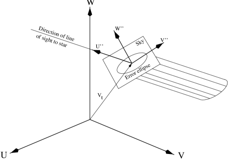
Figure 1: Cylinder in velocity space $(U,V,W)$ determined by the Hipparcos data. The tangential velocity $(\mn@boldsymbol{v}_{t})$ determines the offset from the origin of the central axis of the cylinder. The orientation of the cylinder is determined by the direction of the line of sight. The errors and correlations in the tangential velocity result in an elliptical cross section of the cylinder, which is infinitely long, as no kinematical information in the radial direction is assumed to exist. $(U,V,W)$ can be any set of orthogonal axes in velocity space. It is customary to choose $U$ in the direction of the Galactic centre, $V$ in the direction of Galactic rotation, and $W$ towards the north Galactic pole. The coordinate system $(U^{\prime\prime},V^{\prime\prime},W^{\prime\prime})$ is described in the text.

The direction of the spaghetti axis in velocity space is determined by the position $(\alpha,\delta)$ of a star on the sky. This is the direction in which we lack velocity information. The parallax $(\pi)$ and the proper motion $(\mn@boldsymbol{\mu}=[\mu_{\alpha^{*}},\mu_{\delta}])$ determine the tangential velocity in ${\rm km}~{}{\rm s}^{-1}$, $\mn@boldsymbol{v}_{t}=4.74\mn@boldsymbol{\mu}/\pi$ where $\mn@boldsymbol{\mu}$ is in ${\rm mas}~{}{\rm yr}^{-1}$ and $\pi$ is in mas. The tangential velocity sets the offset of the central axis of the spaghetti from the origin in velocity space (see Fig. 1). The axis $\mn@boldsymbol{s}$ is given by

$${\mn@boldsymbol{s}}={\mn@boldsymbol{v}_{t}}+\lambda{\mn@boldsymbol{\beta}},$$ (1)

where the direction of the line is given by $\mn@boldsymbol{\beta}$, the unit vector in the radial velocity direction, and $\lambda$ is a free scalar parameter. When $\lambda$ is equal to the radial velocity, $\mn@boldsymbol{s}$ equals the star’s spatial velocity. We use an orthogonal velocity coordinate system $(U,V,W)$, with the Solar-system barycentre at the origin, $U$ directed towards the Galactic centre, $V$ in the direction of Galactic rotation, and $W$ towards the north Galactic pole.

The axis $\mn@boldsymbol{s}$ becomes a cylinder in velocity space with an elliptical cross section due to the errors on the tangential velocity. The full covariance matrix of the astrometric parameters is taken into account in the determination of these errors (see ESA 1997, Vol. 1 §1.5.6). The semi-major axis, axis-ratio, and orientation of the ellipse can be calculated using the covariance matrix ${\bf C}$ of the tangential velocity.

For simplicity, we introduce a new coordinate system $(U^{\prime\prime},V^{\prime\prime},W^{\prime\prime})$ such that the $U^{\prime\prime}$-axis coincides with the axis of the cylinder ($\mn@boldsymbol{s}$), and the $V^{\prime\prime}$- and $W^{\prime\prime}$-axis correspond to the major and minor axes, respectively, of the elliptical cross section (see Fig. 1). The surface equation for the cylinder is simplest in this coordinate frame and allows us to define a probability function. The coordinate transformation is done in two parts. First, we apply a rotation, ${\bf T}$, and translation to an intermediate coordinate system $(U^{\prime},V^{\prime},W^{\prime})$. The $U^{\prime}$-axis coincides with the axis of the cylinder, while the $V^{\prime}$- and $W^{\prime}$-axis are not yet aligned with the major and minor axis, respectively. We then translate the origin of the coordinate system to coincide with the tip of the tangential velocity vector. The translation has no effect on the covariance matrix, while the rotation affects ${\bf C}$ as follows

$${\bf\hat{C}}={\bf T}\>{\bf C}\>{\bf T}^{\rm T},$$ (2)

where ${\bf\hat{C}}$ is the covariance matrix in the intermediate coordinate system $(U^{\prime},V^{\prime},W^{\prime})$. ${\bf T}^{\rm T}$ is the transpose of ${\bf T}$. Second, we apply a rotation around the $U^{\prime}$-axis over an angle $\eta$, ${\bf T}_{U^{\prime}}(\eta)$, which can be obtained from the sub-matrix ${\bf\hat{C}}^{\prime}$ consisting of the $V^{\prime}$ and $W^{\prime}$ velocity components. This matrix determines the shape of the elliptical surface of the cylinder. The semi-major axis, $a$, axis ratio, $q$, and rotation angle with respect to the $V^{\prime}$-axis, $\eta$, of the ellipse can be written as

$${\bf\hat{C}}^{\prime} = \left[\begin{array}[]{cc}\sigma_{V^{\prime}}^{2}&\rho\>\sigma_{V^{\prime}}\sigma_{W^{\prime}}\\ \rho\>\sigma_{V^{\prime}}\sigma_{W^{\prime}}&\sigma_{W^{\prime}}^{2}\\ \end{array}\right],$$ (5)

$$a^{2} = \frac{2(1-\rho^{2})\sigma_{V^{\prime}}^{2}\sigma_{W^{\prime}}^{2}}{\sigma_{V^{\prime}}^{2}+\sigma_{W^{\prime}}^{2}-\sqrt{(\sigma_{V^{\prime}}^{2}+\sigma_{W^{\prime}}^{2})^{2}-4(1-\rho^{2})\sigma_{V^{\prime}}^{2}\sigma_{W^{\prime}}^{2}}},$$

$$q^{2} = \frac{a^{4}}{(1-\rho^{2})\sigma_{V^{\prime}}^{2}\sigma_{W^{\prime}}^{2}},$$

$$\eta = \frac{1}{2}\arctan\left(2\rho\frac{\sigma_{V^{\prime}}\sigma_{W^{\prime}}}{\sigma_{V^{\prime}}^{2}-\sigma_{W^{\prime}}^{2}}\right),$$ (6)

where $\rho\equiv\rho_{V^{\prime}}^{W^{\prime}}$. After the rotation we obtain the $(U^{\prime\prime},V^{\prime\prime},W^{\prime\prime})$ coordinate system in which the $V^{\prime\prime}$- and $W^{\prime\prime}$-axis are aligned with the major and minor axes of the error ellipse, respectively. The covariance matrix in the final system can be calculated with eq. (2), using ${\bf T}^{\prime}={\bf T}_{U^{\prime}}(\eta)\>{\bf T}$ instead of ${\bf T}$. The positional accuracy in the Hipparcos Catalogue results in an error in the direction of the cylinder $(\mn@boldsymbol{\beta})$ on the order of $10^{-8}$. We neglect this error.

2.2 The spaghetti density in velocity space

To find the points in velocity space where the number of intersecting cylinders are highest, we define the Spaghetti Density Function in velocity space $(U,V,W)$ as,

$${\rm SDF}(U,V,W)=\sum\limits_{i=1}^{N}\frac{1}{2\pi a_{i}^{\prime 2}q_{i}^{\prime}}\exp\left[-\frac{1}{2}\frac{V^{\prime\prime 2}+W^{\prime\prime 2}/q_{i}^{\prime 2}}{a_{i}^{\prime 2}}\right].$$ (7)

Here $V^{\prime\prime}$ and $W^{\prime\prime}$ are the velocity components in the $(U^{\prime\prime},V^{\prime\prime},W^{\prime\prime})$ system; $a^{\prime}_{i}$ and $q^{\prime}_{i}$ are the semi-major axis and axis ratio of the error ellipse as defined below, respectively, and $N$ is the number of stars. Each term in the summation is interpreted as the probability function for the spatial velocity vector of the corresponding star, and it contains all the kinematic information that the Hipparcos Catalogue provides for that star. The SDF is normalized such that for each cylinder $i$, the integral of the $i^{\rm th}$ component of the SDF over a plane perpendicular to its axis is unity.

The elliptical spaghetti cross section is constrained to have a minimum size, $\sigma_{\rm int}$, thus $a_{i}^{\prime}={\rm MAX}(\sigma_{\rm int},a_{i})$, $b_{i}^{\prime}={\rm MAX}(\sigma_{\rm int},b_{i})$ and $q_{i}^{\prime}=b_{i}^{\prime}/a_{i}^{\prime}$. The reasons for this thickening of the thinnest spaghettis are threefold. First, moving groups have intrinsic velocity dispersions ranging from a few tenths of ${\rm km~{}s}^{-1}$ in open clusters (e.g., Dravins et al. 1997; Perryman et al. 1998) to a few ${\rm km~{}s}^{-1}$ in OB associations (see e.g., Jones & Herbig 1979; Hartmann et al. 1986; Mathieu 1986; Tian et al. 1996). When the mean spaghetti thickness is less than the intrinsic velocity dispersion in a moving group, the typical separation between the axes of the spaghettis is larger than the mean spaghetti thickness. As a result the moving group will not generate a peak in the SDF. This can be solved by artificially increasing the thickness of the spaghettis. Second, the errors on the tangential velocity components are highly correlated due to the way the parallax enters in the conversion of proper motion to velocity. This causes the spaghettis to be very thin in one direction, and depending on the orientation of the spaghettis, the moving group may not generate a peak in the SDF. Third, long period binaries artificially increase the velocity dispersion of a moving group. For binaries with periods longer than the four year observing period of Hipparcos, only part of the orbit was observed and the proper motion may thus be different from that of the centre of mass of the binary system (see Wielen et al. 1997). This effect is especially noticeable for massive equal mass binaries within 200 pc of the Sun and increases the velocity dispersion.

The procedure then is to search for maxima, or peaks, in the SDF. We evaluate the SDF on a Cartesian grid of $4~{}{\rm km}~{}{\rm s}^{-1}$ spacing, and start a steepest gradient search from every grid point which is a local maximum to find the $(U,V,W)$ positions of peaks. This sampling is dense enough to find every peak in the SDF as it is of the same order as the structure in the SDF, whose scale is set by the typical errors in tangential velocity and the internal dispersion, $\sigma_{\rm int}$.

2.3 Peak significance

In order to assign a statistical significance to peaks in the SDF obtained from the data, it is necessary to build the ‘null hypothesis’ and obtain its expected distribution of peaks. The ideal null hypothesis is the Hipparcos database that would be obtained when observing a Galaxy in which no moving groups exist.

Ideally, we would do a series of Monte Carlo experiments in which several random realizations of the Hipparcos Input Catalogue are generated from the null model. The resulting observed properties would be reduced with the techniques used for the real data to derive the final astrometric quantities and their associated uncertainties and correlations. Such a procedure is enormously complex, and for this, a suitable approximate null hypothesis must be found. Therefore, we decided to generate random realizations of the proper motion components alone for the stars in the real data set, leaving all other quantities fixed. We use the Schwarzschild ellipsoid as the local velocity distribution for our null model of the Galaxy without moving groups. The first and second moments, and the vertex deviation were taken from an analysis of local Hipparcos main-sequence stars by Dehnen & Binney (1998). This model also includes their values of the Solar motion and asymmetric drift. The Oort constants for the Galactic rotation are taken from Feast & Whitelock (1997). This procedure should produce a reasonable approximation, since it is only the information that bears the signature for grouping in velocity space, the proper motion information, that has been obtained from the null model, leaving everything else intact. The kinematic model is based on an unbiased sample of main-sequence stars within 100 pc of the Sun. Stars at larger distances, giants, and super giants may have different kinematic properties and using those of the nearby main-sequence stars in the simulations results in some systematic effects in the null hypothesis. For more details on this procedure see §3.4 in de Zeeuw et al. (1999).

The expected distribution of peak heights is obtained from 100 Monte Carlo experiments and the significant peaks in the real data are obtained by direct comparison. An additional difficulty comes from the fact that the variation in density of stars in velocity space produces a changing background in the SDF, thus making the statistical significance of a peak dependent on position in velocity space. To address this problem, we obtain the median SDF from the set of all Monte Carlo realizations of the null model sampled on a grid of 4 ${\rm km~{}s}^{-1}$ spacing. The median SDF is subtracted from both the SDF of the real data and of the experiments.

2.4 Membership

Having located a significant peak in the SDF we determine membership for all stars. The fraction of the spaghetti which lies within a sphere of radius $R_{s}$ in velocity space centred on the peak is taken as a measure of membership. This fraction is evaluated using the volume integral of the spaghetti over the sphere. We take

$$R_{s}=\sqrt{\sigma_{\rm int}^{2}+\sigma_{\rm median}^{2}},$$ (8)

so that $R_{s}$ is a measure of the extent of the peak resulting from the median error on the tangential velocity, $\sigma_{\rm median}$, and the estimated internal velocity dispersion, $\sigma_{\rm int}$. $\sigma_{\rm median}$ is the typical thickness of a spaghetti and is set to the median of the spaghetti semi-major axes for which the SDF is calculated. $\sigma_{\rm median}$ can also be calculated for stars in a certain distance range if some a priori knowledge on the moving group distance is available, and can be improved upon by iteration. The integral over the $U^{\prime\prime}$-axis of the volume integral can be done analytically. This leaves the following double integral

$$S = \frac{1}{2R_{s}}\,\int\!\!\!\int_{C}2\sqrt{R_{s}^{2}-(V^{\prime\prime}-V^{\prime\prime}_{0})^{2}-(W^{\prime\prime}-W^{\prime\prime}_{0})^{2}}\times$$ (9)

$$\quad\quad\frac{1}{2\pi a^{2}q}\,\exp\left[-\frac{1}{2}\frac{V^{\prime\prime 2}+W^{\prime\prime 2}/q^{2}}{a^{2}}\right]dW^{\prime\prime}dV^{\prime\prime},$$

where $a$ is the semi-major axis of the spaghetti and $q$ the axis ratio. Here $C$ is the surface enclosed by a circle centred on $(V^{\prime\prime}_{0},W^{\prime\prime}_{0})$ with radius $R_{s}$. $(U^{\prime\prime}_{0},V^{\prime\prime}_{0},W^{\prime\prime}_{0})$ are the coordinates of the peak. As a spaghetti is normalized to unity in the plane perpendicular to its axis, we divided the integral by $2R_{s}$ for $S$ to range between 0 to 1.

$S$ can be interpreted as a conditional probability. However, it is not straightforward to compare conditional probabilities, wich makes them difficult to use for membership assignment. Therefore we consider as members only those stars for which $S$ exceeds a threshold value $S>S_{\rm min}$ (see discussion in §3.2.2). $S$ depends on distance; for two spaghettis with exactly the same central axis but different thickness, $S$ will be smallest for the thickest spaghetti. Since the thickness of the spaghettis increases with increasing distance — the errors on the tangential velocity increase — $S$ will decrease and thus depends on distance. Any selection method which includes the parallax suffers from this effect.

3 Tests on synthetic data

We now describe tests of the Spaghetti method on synthetic data consisting of a field star population and one moving group, and one data set containing field stars and two moving groups.

3.1 Synthetic data sets

We use the procedure described in §2.3 to generate a sample of field stars. We draw a star from the Hipparcos Catalogue and, if the star lies in the requested field (see Table 1), replace its observed proper motion with a proper motion consistent with our kinematic model for the Solar neighbourhood (§2.3). Again, all other information, e.g., position, parallax, errors, and correlations, are not altered.

We generate 20 random realisations for each of 24 different setups in which the field centre and distance of the cluster are varied. For each distance we adopt a different field size and different numbers of field and cluster stars (see Table 1). The total number of stars is chosen such that there are about 3 stars per square degree, as in the Hipparcos Catalogue. Distant clusters subtend smaller angles on the sky, allowing a smaller field, and as only the brightest members are visible the number of cluster stars decreases with distance. The adopted numbers are consistent with those found by de Zeeuw et al. (1999) for the nearby OB associations. Varying the Galactic longitude of the field centre allows us to investigate the effect of Solar motion and Galactic rotation. The positions of the moving group members are drawn from a sphere of constant density with a radius of 15 pc, which is a typical size for a moving group (see e.g., Blaauw 1991; Perryman et al. 1998). The velocity of each star consists of four components: Solar motion, Galactic rotation, streaming velocity, and an internal velocity dispersion. The streaming velocity is defined as the spatial velocity of a moving group with respect to its own standard of rest. The Solar motion and Galactic rotation are the same as those used for the field stars. The streaming velocity, which is different in each data set, is drawn uniformly from a sphere of 10 ${\rm km}~{}{\rm s}^{-1}$ radius. This is a reasonable representation of the velocity distribution of molecular clouds, which have a typical dispersion of 6–8 km s^-1 (see e.g., Dickey & Lockman 1990; Burton, Elmegreen & Genzel 1992). The internal velocity dispersion is represented as a Gaussian with $2~{}{\rm km}~{}{\rm s}^{-1}$ standard deviation in each coordinate. Position and velocity are then converted into position on the sky, parallax, and proper motion. We then perturb the parallax and proper motion with errors drawn from a Gaussian error distribution with 1 mas and 1 ${\rm mas}~{}{\rm yr}^{-1}$ standard error, respectively.

Table 1: The 24 different setups of the synthetic data sets used to test the Spaghetti method. For every setup 20 random realizations are created resulting in a sample of 480 data sets. Four distances are used for each of the following 6 field centres: $\ell=0^{\circ}\!,60^{\circ}\!,120^{\circ}\!,180^{\circ}\!,240^{\circ}\!,300^{\circ}\!$ and $b=0^{\circ}\!$. The other characteristics of each data set, such as field size and the number of field and cluster stars, depend on the distance. The total number of stars per field is consistent with 3 stars per square degree, as in the Hipparcos Catalogue. The size of the simulated cluster is 15 pc in radius for each data set.

Distance	Field stars	Cluster stars	Field size
pc	#	#
150	1000	200	$20^{\circ}\times 20^{\circ}$
300	1575	100	$15^{\circ}\times 15^{\circ}$
450	1250	150	$10^{\circ}\times 10^{\circ}$
600	1275	125	$10^{\circ}\times 10^{\circ}$

Figure 2: The four panels show the peak height distribution for 8 synthetic data sets for the $(\ell,b)=(0^{\circ}\!,0^{\circ}\!)$ field at 4 different distances each. The top histogram in each panel shows the distribution of peak heights in the 100 Monte Carlo realizations for the null hypothesis, no moving groups, of the synthetic data sets. The ticks on the ordinate have a spacing of two decades, at 1 and 100 peaks. The second histogram is the peak height distribution for the null hypothesis after subtraction of the SDF background. The following 8 histograms give the peak height distribution, after the SDF background has been subtracted, for the first 8 of the 20 synthetic data sets of these particular setups. The peak corresponding to the moving group is indicated by an arrow. The dotted line indicates a 99.9 per cent chance of finding a smaller peak height. See text for further explanation.

3.2 Results

3.2.1 Peak significance

The distributions of peak heights in the synthetic data sets for the direction $(\ell,b)=(0^{\circ}\!,0^{\circ}\!)$, and distances of $150$, $300$, $450$, and $600$ pc are shown in Fig. 2. The top histogram in each panel shows the combined peak height distribution for the 100 Monte Carlo simulations of the null hypothesis before subtraction of the SDF background. Although most peaks have small peak heights there is a plateau at larger values. After subtracting the SDF background, the peak height distribution, shown in the second histogram from the top, is nearly exponential. The Monte Carlo peak height distribution is the result of chance intersections of spaghettis in velocity space; extending it to higher peak values would require an order of magnitude more simulations. With current workstations this is not practical. This makes it difficult to assign a realistic significance value to peaks higher than 0.5. The dotted lines in Fig. 2 indicate the 0.1 per cent chance for a peak of at least that peak height to be generated in a data sample of field stars only.

The following 8 histograms in each panel show the peak hight distribution, corrected for the SDF background, for the first 8 of the 20 realisations of these particular situations. In each panel the peak distribution follows the null hypothesis peak distribution for the small peak values, $\la 0.1$. However, the panels also show one or more peaks around 3.0, 1.0, 0.4, and 0.2 for 150, 300, 450, and 600 pc, respectively. In all cases one of these peaks corresponds to the moving group, indicated by the arrows. These peaks stand well clear from the Monte Carlo peak distribution. The height of the moving group peak decreases with distance. More distant clusters are less significant (§2.2). Furthermore, the peak height also depends on the number of moving group stars present in the data set, the velocity dispersion, and the data quality.

The Spaghetti method sometimes finds more than one significant peak in a synthetic data set containing only one moving group. This is due to the parallelism of the spaghettis — as we are looking at a specific field on the sky all spaghettis have similar directions. This causes the moving group peak in the SDF to be stretched in the radial direction (see also Fig. 8 panel [j]). Small random peaks generated by the field star population superposed on this larger peak will be classified as significant based on peak height only. In general, the highest of this set of peaks is centred on the moving group velocity, while the significant artificial peaks are all aligned with the line of sight direction passing through the moving group velocity. This distinguishes artifical peaks from multiple moving groups.

3.2.2 Membership threshold and success rate

Fig. 3 shows, for one of the fields, $(\ell,b)=(0^{\circ}\!,0^{\circ}\!)$, the fraction of selected field and cluster stars versus $S_{\rm min}$ (see §2.4). We used the stars within a distance range of 200 pc centred on the cluster distance to determine $\sigma_{\rm median}$ and hence $R_{s}$ (see §2.4). We used $\sigma_{\rm int}=2~{}{\rm km~{}s}^{-1}$. A sharp increase can be seen in the fraction of selected field stars at $S_{\rm min}\approx 0.1$. On the other hand, the number of selected cluster stars rises steadily for decreasing $S_{\rm min}$. This trend led us to pick $S_{\rm min}=0.1$ as the border-line between member and non-member. It is clear that the value of $S_{\rm min}$ can be adjusted for specific problems. The results do not depend sensitively on position on the sky.

Figure 3: Fraction of moving group, closed circles, and field, open circles, stars selected by the Spaghetti method as a function of membership threshold $S_{\rm min}$. These results are for the field $(\ell,b)=(0^{\circ}\!,0^{\circ}\!)$ and $\sigma_{\rm int}=2~{}{\rm km~{}s}^{-1}$. The distance of the cluster is 150, 300, 450, and 600 pc with the corresponding properties as described in Table 1. The figure displays the median of 20 random realizations and the errors are estimated by the interquartile range.

The threshold value $S_{\rm min}=0.1$ leads to the selection of 90/4, 93/11, 88/17, and 84/45 per cent of the cluster/field stars for 150, 300, 450, and 600 pc respectively (see Fig. 4). These success rates can be compared with those obtained by the refurbished convergent point method of de Bruijne (1999) using similar simulations. He finds 80/20, 75/15, 50/13, and 52/13 per cent of the cluster/field stars for the same distances. The percentage of selected cluster stars is higher for the Spaghetti method and remains roughly constant over the sampled distance range. The percentage of selected field stars in the Spaghetti method increases with distance, especially for the most distant data sets, whereas in the convergent point method this percentage remains constant. Only for the most distant data sets does the Spaghetti method select many more field stars than the convergent point method. However, the number of selected cluster stars remains above 80 per cent. Although the contamination by field stars increases with distance, the Spaghetti method samples a larger fraction of the cluster than the convergent point method. The increase in selected field stars with distance is due to the increasing tangential velocity errors, corresponding to an increase in the thickness of the spaghettis. This results in a larger value of $R_{s}$, the radius of the sphere in velocity space used for the membership determination (see §2.4). The fraction of selected cluster stars shows the same trend with $S_{\rm min}$ at any distance because the typical thickness of these spaghettis determines $R_{s}$, while the number of selected field stars increases because $R_{s}$ is not related to those stars. Field stars are located at all distances and their spaghettis span a whole range of thicknesses. Especially the nearest field stars, having thin spaghettis, will be selected more easily if $R_{s}$ is large. This also puts a limit, $\sim$750 pc, on the distance at which the Spaghetti method can be used reliably using the Hipparcos data. The typical error on the tangential velocity at 750 pc, $\sim$$20~{}{\rm km}~{}{\rm s}^{-1}$, is of the same order as the large scale structure in velocity space. Other diagnostics, e.g., the parallax distribution or photometric information of the selected stars or a combination with another selection method (see e.g., de Zeeuw et al. 1999), can be used to lower the number of selected field stars.

Figure 4: Success rate of the Spaghetti method compared to the classical convergent point method (by de Bruijne 1999) as a function of distance. The filled circles and triangles represent the fraction of cluster stars found in the Monte Carlo simulations by the Spaghetti and convergent point method, respectively. The open circles and triangle represent the fraction of field stars found for both methods.

Fig. 5 shows the success rate of the Spaghetti method as a function of distance, the value of $\sigma_{\rm int}$, and the percentage of selected cluster members. It shows in how many of the data sets we select a certain percentage of cluster stars, e.g., at a distance of 150 pc and $\sigma_{\rm int}=2~{}{\rm km~{}s}^{-1}$ we find 85 per cent of the cluster members in 50 per cent of the data sets. It shows that the value for $\sigma_{\rm int}$ is not important in the member selection for moving groups beyond $\sim$300 pc. This is expected because, at these distances, the errors on the tangential velocity dominates $R_{s}$ (eq. 8). For moving groups at smaller distances it is important to know the internal velocity dispersion. The top panel in Fig. 5 shows that if $\sigma_{\rm int}$ is equal to e.g., 1.5 times the velocity dispersion in the simulated data sets the success rate is much better than when $\sigma_{\rm int}$ is equal to this velocity dispersion. As it is difficult to obtain reliable estimates for the internal velocity dispersions in moving groups it is best to use a somewhat large value for $\sigma_{\rm int}$ for the nearest moving groups. Fig. 5 also shows that the success rate decreases with distance. This is due to the increasing errors on the tangential velocities which decrease the ‘resolving power’ of the Spaghetti method at larger distance. The Spaghetti method will never find all moving group members because there will always be stars in the wings of the velocity distribution that fall outside $R_{s}$. This argument applies to any selection process for moving groups, and results in a characteristic number of cluster stars we find in a typical data set of: $\sim$90 per cent for 150 to 300 pc and $\sim$85 and $\sim$80 per cent for 450 and 600 pc, respectively.

Figure 5: The panels show the success rate of the Spaghetti method as a function of the percentage of selected cluster members, using $S_{\rm min}=0.1$ (i.e. for 150 pc and $\sigma_{\rm int}=2~{}{\rm km~{}s}^{-1}$ we find 50 per cent of the cluster members in all data sets and 85 per cent in half of the data sets). The panels are divided according to distance. The solid lines indicate the results of the member selection for $\sigma_{\rm int}=2$ km s^-1, equal to the internal velocity dispersion in the simulations. The dotted and dashed lines indicate the results for $\sigma_{\rm int}=1$ and 3 km s^-1, respectively. The lower three panels show that for these distances $\sigma_{\rm int}$ is not important in the member selection; the errors on the tangential velocity are larger than the velocity dispersion. For moving groups at $\sim$150 pc, $\sigma_{\rm int}$ is important and the panel shows that its value should be taken somewhat larger than the internal velocity dispersion.

Figure 6: The relative difference in tangential velocity $\Delta V_{T}/V_{T}$ of the synthetic moving cluster and the tangential velocity found by the Spaghetti method, as a function of distance. The filled dots and error bars are the median and interquartiles respectively for 20 data sets. The open dots, shifted by 10 pc, show the bias in $\Delta V_{T}/V_{T}$ as present in the Monte Carlo simulations of only cluster stars, so no field contamination is present. The 6 panels show the results for the line of sight indicated in each panel. The dotted lines indicate the predicted bias in tangential velocity resulting from the use of the parallax in its calculation.

3.2.3 Velocity

Apart from a list of members and non-members, the Spaghetti method produces the $(U,V,W)$ velocity of the moving group — the velocity of the peak in the SDF. The predicted radial velocity will have the largest uncertainty. When a moving group is confined to a small region on the sky, it is difficult to find the precise radial velocity due to the parallelism of the spaghettis which stretch the peak in the radial direction (see e.g., Fig. 8 panel [j]). If however, a moving group covers a large fraction of the sky the spaghettis contributing to the peak come from a large range of directions, and the predicted radial velocity will be much better constrained (see e.g., the Cas–Tau association covering more than 100${}^{\circ}\!$ by 60${}^{\circ}\!$ on the sky [§7.2 in de Zeeuw et al. 1999]).

Fig. 6 shows the relative difference in the tangential velocity between that of the moving group and the one found by the Spaghetti method, $\Delta V_{T}/V_{T}=(V_{\rm spaghetti}-V_{T})/V_{T}$. Here $V_{T}$ is the tangential part of the total moving group velocity used in the simulations, representing the group’s streaming motion, the Solar motion, and Galactic rotation. $V_{\rm spaghetti}$ is the tangential velocity found by the Spaghetti method. For every direction, $\Delta V_{T}/V_{T}$ increases with distance. At 600 pc in the direction $\ell=300^{\circ}\!$ the offset is as large as 20 ${\rm km}~{}{\rm s}^{-1}$. This trend in $\Delta V_{T}/V_{T}$ is due to a bias introduced by the parallax in the calculation of the tangential velocity, and is similar to the bias in distance when calculated as $1/\pi$, see Smith & Eichhorn (1996) and Brown et al. (1997). To estimate the magnitude of the tangential velocity bias we redid the Monte Carlo simulations of the synthetic data sets without the field stars (indicated in Fig. 6 by the open dots). The tangential velocity differences we find in these simulations includes the true bias but excludes any effect introduced by the field star population. We also calculated the proper motion due to Solar motion and Galactic rotation in the six different directions as a function of distance. Combined with the biased distances, as described by Brown et al. (1997), this gives another measure of the bias in tangential velocity, indicated by the dotted line in Fig. 6 which follows the points rather well. The most distant points in the directions $\ell=60^{\circ}\!$ and $120^{\circ}\!$ do not follow the trend due to the bias in parallax only. This could be due to the combined effects of Solar motion and Galactic rotation which results in very small, almost zero, tangential velocity for these directions and distances. The effects due to the selection method probably dominate in these cases.

The spread in $\Delta V_{T}/V_{T}$ we find is of the same magnitude as the typical error in the tangential velocity, and indicated in Fig. 6 by the error bars. The spread in radial velocities is much larger and in some cases differs by as much as 100 ${\rm km}~{}{\rm s}^{-1}$ from the real radial velocity.

Another important characteristic of the Spaghetti method is that a simple linear expansion or contraction of a moving group will influence the radial velocity found by our method. This is inherent to the fact that we use proper motions and parallaxes only. Without accurate radial velocities ($\sigma_{v_{\rm radial}}<{\rm a~{}few}~{}{\rm km}~{}{\rm s}^{-1}$) it is impossible to distinguish an expanding moving group which is stationary with respect to the observer from a moving group which is moving towards the observer — the so-called perspective effect — (Blaauw 1964). Thus, when using the predicted radial velocity of a moving group it is important to keep in mind that part of the radial velocity might be due to expansion or contraction.

3.3 Multiple groups

Figure 7: The bottom histogram in the bottom panel shows the significant peaks, indicated by the arrows, corresponding to the all-sky (1) and the confined (2) moving group present in this particular synthetic data set. The top and middle histogram are the Monte Carlo peak distribution before and after background subtraction (§2.3). The ticks on the ordinate are spaced every two decades. The top panel shows the selected stars of the all-sky moving group, filled circles are genuine members and open circles are selected field stars. The small dots are the remaining stars in the data set. The middle panel is identical to the top panel but now shows the results of the second moving group. 95 genuine members are located around $(\ell,b)=(200^{\circ}\!,10^{\circ}\!)$.

We also apply the Spaghetti method to a synthetic data set which contains two moving groups. The data set consists of 5000 field stars, one group of 100 stars at 200 pc in the direction of $(\ell,b)=(200^{\circ}\!,10^{\circ}\!)$ with a radius of 15 pc, and a group of 100 stars covering the whole sky, i.e., a distance of 20 pc in the direction $(\ell,b)=(0^{\circ}\!,0^{\circ}\!)$ and a radius of 100 pc. Both moving groups have a small streaming velocity and a velocity dispersion of 2 km s^-1. The field stars are generated using the procedure described in §2.3. We find several significant peaks for this data set (Fig. 7, bottom panel), using $\sigma_{\rm int}=2$ km s^-1. The most significant peak corresponds to the all-sky group while one of the other peaks coincides with the velocity of the second moving group, indicated with 1 and 2 in Fig. 7, respectively. Both peak velocities agree within 0.5 km s^-1 with those of the moving groups. The other significant peaks are phantom peaks generated by both groups (cf. §3.2.1). Using all stars between 50 and 150 pc, we obtain $\sigma_{\rm median}=4.20$ km s^-1, resulting in the selection of 211 stars as member of the all-sky group (Fig. 7, top panel). Of these, 98 are classified correctly. We select 446 members for the other group ($\sigma_{\rm median}=7.02$ km s^-1 for all stars between 150 and 250 pc) of which 95 are genuine members (Fig. 7, middle panel).

In conclusion, the Spaghetti method succeeds in the detection of both moving groups and in the selection of more than 90 per cent of their members. The only drawback, caused by the large field of view, are the large numbers of misidentified members: 113/211 for the all-sky group and 351/446 for the other. The large fraction of selected field stars will make any analysis of all-sky moving groups extremely difficult; only accurate age and chemical abundance information may shed further light on the physical existence of such groups. However, the method does reduce the number of stars of interest considerably, which makes follow-up studies feasible.

Table 2: Results of the member selection for the Hyades open cluster by the Spaghetti method compared to Perryman et al. (1998; P98). The table shows the number of stars considered as member by P98 for different confidence intervals, 68.3, 95.4, and 99.7 per cent (corresponding to the 1, 2, and 3$\sigma$ confidence intervals), for all members and for the members within 10 and 20 pc of the cluster centre of mass. The P98 results are compared to the members found by the Spaghetti method, SP, and the difference between P98 and SP, P98 - SP, and SP - P98 respectively.

	$\leq 3\sigma$			$\leq 2\sigma$			$\leq 1\sigma$
	Total	r $<$ 10 pc	r $<$ 20 pc	Total	r $<$ 10 pc	r $<$ 20 pc	Total	r $<$ 10 pc	r $<$ 20 pc
P98	218	134	180	190	131	170	162	121	150
P98 - SP	56	11	29	30	8	19	7	0	3
SP	168	124	154	168	124	154	168	124	154
SP - P98	6	1	3	8	1	3	13	3	7

4 Tests on the Hyades and IC2602

Below, we discuss results obtained by the Spaghetti method for two moving groups: the well-studied Hyades open cluster, and the open cluster IC2602. Another application of the Spaghetti method, in combination with the refurbished convergent point method of de Bruijne (1999), can be found in de Zeeuw et al. (1999), who used the method to improve and extend the membership lists for 12 nearby OB associations.

4.1 The Hyades

Ever since its discovery as a moving group, the Hyades open cluster has been at the centre of attention in studies of open cluster evolution, distance calibration, and stellar evolution models. Here we compare the most recent membership determination by Perryman et al. (1998, hereafter P98) to stars selected by the Spaghetti method.

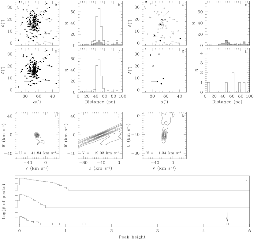
Figure 8: Panel (a) shows the positions and proper motions of the Hyades members as selected by Perryman et al. (1998; P98). The most significant members (within the 68.3 per cent confidence level) of P98 are denoted by black dots. The remaining stars lying within the 68.3 per cent and 99.73 per cent confidence level are denoted by grey dots. Panel (b) shows a histogram of the distances for all P98 members. The grey histogram indicates the less significant members. The members with low significance are spatially less concentrated than the more significant members. Panel (c) shows the positions and proper motions of the P98 members which are not selected by the Spaghetti method; most of them have low significance and are located outside the main cluster, see the distance histogram in Panel (d). The colour scheme is the same as in Panel (a). Panel (e) shows the positions and proper motions of the Hyades members selected by the Spaghetti method. The corresponding distance histogram is shown in Panel (f). The positions and proper motions of the stars selected as member by the Spaghetti method which are not a P98 member are shown in Panel (g). Panel (h) shows the distance distribution of these stars. The Panels (i), (j), and (k) show slices through the SDF for the peak corresponding to the Hyades open cluster. The peak velocity is $(U,V,W)=(-41.84,-19.03,-1.34)~{}{\rm km}~{}{\rm s}^{-1}$, where $(U,V,W)$ are the Galactic Cartesian velocity coordinates. Panels (i) and (k) show a clear peak and a broader feature centred on the Solar motion. The elongated peak in Panel (j), stretched in the radial direction, is caused by the parallelism of the individual spaghettis. In general this effect results in a large uncertainty on the predicted radial velocity for the moving group. However, due to the large solid angle subtended by the Hyades on the sky and its significant peculiar velocity this is not a problem for the Hyades. Panel (l) shows the significance of the peak created by the Hyades in the SDF: the top histogram shows the peak distribution for a Monte Carlo simulation as described in §2.3, the second histogram is the peak height distribution for the same simulation but after the SDF background has been subtracted. The bottom histogram shows the peak height distribution for the Hyades data sample after subtraction of the Monte Carlo background. The ticks on the ordinate are spaced every two decades. The peak corresponding to the Hyades moving group is indicated with an arrow.

P98 base membership of the Hyades on the three-dimensional velocity of a star and the three-dimensional centre-of-mass motion of the cluster. A star is considered as member if these two are consistent within their associated statistical errors within the 99.73 per cent confidence level. For stars with unknown radial velocity membership is based on the tangential velocity only. P98 find 218 members of which 21 do not have a measured radial velocity. 134 of the 218 are located within 10 pc of the cluster centre of mass and 180 within 20 pc. The tidal radius of the cluster is 9 pc. P98 find a centre-of-mass velocity, with respect to the Sun for the 134 members within 10 pc, of $(U,V,W)=(-41.70\pm 0.16,-19.23\pm 0.11,-1.08\pm 0.11)$ ${\rm km}~{}{\rm s}^{-1}$ and a distance of $46.34\pm 0.27$ pc.

We apply the Spaghetti method to all Hipparcos stars in the field $2^{\rm h}15^{\rm m}<\alpha<6^{\rm h}5^{\rm m}$ and $-2^{\circ}\!<\delta<35^{\circ}\!$ with parallaxes larger than 10 mas. This is the same sample used by P98. We take the internal velocity dispersion, $\sigma_{\rm int}$, to be 2.0 ${\rm km}~{}{\rm s}^{-1}$. This value is larger than the 0.3 ${\rm km}~{}{\rm s}^{-1}$ found by P98. However, when combined with the median error (1.64 ${\rm km}~{}{\rm s}^{-1}$) for stars between 25 to 65 pc from the Sun, this results in a radius for the sphere of interest of $R_{s}=2.58~{}{\rm km}~{}{\rm s}^{-1}$, similar to the $1\sigma$ errors in the centre-of-mass motion for the Hyades (eq. 17 and fig. 16 of P98).

The Hyades cluster generates a significant peak in the SDF (see Fig. 8 panels [i]–[l]). The peak stands well clear from the background peak distribution expected for a similar data set without moving groups (see §§2.3 and 3.2.1). The other 3 significant peaks in Fig. 8 panel [l] are also generated by the Hyades. These are random peaks superposed on that of the cluster. We find a velocity for the Hyades from the position of the peak in the SDF of $(U,V,W)=(-41.84,-19.03,-1.34)$ ${\rm km}~{}{\rm s}^{-1}$ with respect to the Sun. This is within 0.3 ${\rm km}~{}{\rm s}^{-1}$ equal to the velocity found by P98; their result for stars within 10 pc of the cluster centre.

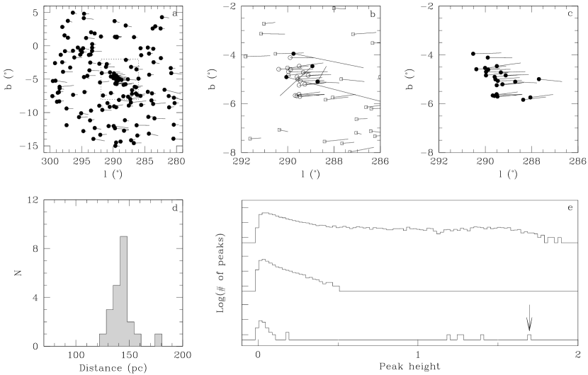
Figure 9: Panel (a): Positions and proper motions of 156 stars classified as member of IC2602. Besides the clearly visible cluster at $(\ell,b)=(289^{\circ}\!,-5^{\circ}\!)$ the Spaghetti method also selects a large number of field stars. Panel (b) shows a $6^{\circ}\!\times 6^{\circ}\!$ field centred on IC2602, also indicated by the dashed lines in panel (a). The open symbols show the 42 stars selected by the Spaghetti method. The 19 open circles are also in the membership lists of Whiteoak (1961) and Braes (1962). The 4 filled circles are Whiteoak and Braes members, not confirmed by the Spaghetti method. The stars located on the edge of this field (square dots) are, all but 4, considered as field stars. The resulting 23 IC2602 members are shown in panel (c). Panel (d) displays a distance histogram for these stars. Panel (e) shows the peak significance of IC2602 (arrow) as in Fig. 8.

Using a membership threshold of $S_{\rm min}=0.1$ (see §3.2.2) we select 168 stars as belonging to the Hyades. Of these, 6 are not in the member list of P98 and 56 of the 218 P98 members are not selected by the Spaghetti method (see also Table LABEL:tab:hyades). A comparison of the position, proper motion, and parallax distribution for both approaches is presented in Fig. 8. The 6 stars selected by the Spaghetti method but not by P98 do not show any clustering in position on the sky and in distance; and are most likely all field stars. Only one of these 6 stars (HIP20693) is listed as a classical member of the Hyades and was rejected by P98 on the basis of its radial velocity. Most of the 56 P98 members not found by the Spaghetti method have a membership significance outside the 68.3 per cent confidence level (table 2 in P98) and are mostly located further than 20 pc from the centre of mass (see Table LABEL:tab:hyades and Fig. 8).

In conclusion, the Spaghetti method selects the majority of the P98 Hyades members, where the number of Spaghetti members missed by P98 is less than the P98 members missed by the Spaghetti method. The difference in membership lists mostly concerns stars having a low significance in the P98 analysis.

4.2 IC2602

IC2602 is a young open cluster centred on the second magnitude star $\theta$ Car. Membership for the brightest stars, of spectral types A0 and earlier, was determined by Whiteoak (1961) and Braes (1962) resulting in a total of 46 candidate members, at a distance of $\sim$155 pc. Only recently, using photometric, spectroscopic, and X-ray information, has it become possible to assign membership for fainter stars, $V\sim 10$ to $\sim$18 mag. This resulted in about 50 additional members (see e.g., Prosser, Randich & Stauffer 1996; Stauffer et al. 1997; Foster et al. 1997; Randich et al. 1997). The age estimates range from 8 Myr, based on the ages of the brightest members (Whiteoak 1961; Braes 1962), to 30 Myr, based on isochrone fits to the low mass members (Stauffer et al. 1997). As most of the fainter members of IC2602 are not listed in the Hipparcos Catalogue we compare our results to those of Whiteoak and Braes. Only 24 of their 46 members are contained in the Hipparcos Catalogue.

We apply the Spaghetti method to all stars in the Hipparcos Catalogue in the field $280^{\circ}\!<\ell<300^{\circ}\!$ and $5^{\circ}\!<b<-15^{\circ}\!$ centred on IC2602. This field also contains part of the Lower Centaurus Crux subgroup of the Sco OB2 association at $118\pm 2$ pc (de Zeeuw et al. 1999). These authors showed that HIP52357, proposed as member of IC2602 by both Whiteoak (1961) and Braes (1962), is a member of this association. We exclude this star in the following discussion. Of the 1958 stars in the field 104 have $\pi\leq 0$ and are not included in the selection. We use all stars with distance between 50 and 250 pc to obtain a value of $\sigma_{\rm median}$ (2.9 km s^-1), and we adopt 2 ${\rm km}~{}{\rm s}^{-1}$ for the internal dispersion, $\sigma_{\rm int}$. The method finds 156 stars related to a significant peak in the SDF (see Fig. 9 panels [a] and [e]) at a velocity $(U,V,W)=(-12.6,-7.2,-0.5)~{}{\rm km}~{}{\rm s}^{-1}$. Due to the large field we select a considerable number of field stars having indistinguishable kinematics from the moving group (Fig. 9 panel [a]). However, IC2602 is clearly visible. Note that the Spaghetti method picks up a moving group of $\sim$30 stars out of 1854. In the following we only consider the stars in a $6^{\circ}\!\times 6^{\circ}\!$ field centred on $(\ell,b)=(289^{\circ}\!,-5^{\circ}\!)$.

Table 3: Hipparcos identifiers and $S$ values for the 23 IC2602 members

HIP	$S$	HIP	$S$	HIP	$S$	HIP	$S$
51131	0.67	51203	0.66	51300	0.42	51794	0.23
52059	0.78	52116	0.60	52132	0.86	52160	0.89
52171	0.48	52221	0.68	52261	0.80	52293	0.90
52328	0.88	52370	0.88	52419	0.82	52502	0.71
52678	0.67	52701	0.68	52736	0.93	52815	0.64
52867	0.40	53016	0.84	53330	0.42

We select 42 stars in this field of which 19 are also in the lists of Whiteoak and Braes (Fig. 9 panel [b]). Only 4 of the Whiteoak and Braes members are not selected by the Spaghetti method. The astrometric parameters for one of these, HIP517979, are a solution for the B and C component of the triple system CCDM 10350-6408 of which component A, HIP51794, is selected as member of IC2602. The complex configuration of this triple system might have caused the Hipparcos solution to be in error as is also indicated by fields H29 and H30 in the Hipparcos Catalogue. The other three stars, HIP52178, HIP52216, and HIP52839, all have good solutions. The remaining 23 stars are almost all situated near the edge of the field and at distances larger than 200 pc. Only four of these stars, HIP51131, HIP51202, HIP51300, and HIP53330, the ones closest to the cluster, are considered as genuine members of IC2602. We consider these four, plus all stars selected by Whiteoak (1961), Braes(1962) as well as the Spaghetti method — 23 stars in total — as genuine IC2602 members (see Table 3 and Fig. 9 panel [c]).

Although we did not use the parallaxes directly in the selection process the distance distribution of the IC2602 members shows a sharp peak, indicating that the cluster is not only confined in velocity space but also in configuration space (Fig. 9 panel [d]). We find the mean distance of the 23 cluster members, using the mean parallax of the cluster and corrected for the known biases as described in de Zeeuw et al. (1999), to be $145\pm 4$ pc. This is $\sim$10 pc closer than the previous estimates of Whiteoak and Braes.

5 Summary and discussion

We have presented a new method to identify moving groups, and select their members, based on position, proper motion, and parallax information only, i.e., using the Hipparcos Catalogue. The astrometric parameters and their errors define a probability distribution function represented by a cylinder with an elliptical cross section in velocity space. Moving group stars, having the same spatial velocity, produce an overdensity in the combined probability function, the SDF, in velocity space. Assessing the significance of these peaks allows for the detection of moving groups and hence the selection of members.

The characteristics of the method have been tested on synthetic data. Typically the Spaghetti method finds $\sim$85 per cent of the synthetic cluster members for distances out to 600 pc. The contamination by field stars increases rapidly after 450 pc which makes cluster detection impossible beyond $\sim$750 pc. This is due to the typical error on the Hipparcos parallaxes, $\sim$1 mas, corresponding to errors in the tangential velocity of $\sim$20 km s^-1 at 750 pc, which is of the same order as the structure in velocity space. The method has primarily been developed to identify moving groups in the Hipparcos database. Any further analysis should take into account the selection effects and kinematic biases which originate from the construction of the Catalogue. For example, the Catalogue is biased towards high proper motion stars although it has a formal absolute proper motion cut off of zero.

Results were presented for the Hyades and IC2602 open clusters. For the Hyades we find most of the members proposed by Perryman et al. (1998). The differences between the two membership lists generally concern P98 members of low significance, most likely field stars. Furthermore, we confirm most of the bright IC2602 members as found by Whiteoak (1961) and Braes (1962), and add four new ones.

The typical errors of $\sim$1 mas in proper motion and parallax prevent identification of moving groups in the Hipparcos Catalogue more distant than $\sim$750 pc from the Sun. The future space astrometry mission GAIA (see e.g., Lindegren & Perryman 1996) aims at observing positions, parallaxes, and proper motions with accuracies of $10~{}\mu$as and $10~{}\mu{\rm as}~{}{\rm yr}^{-1}$, respectively, at $V\sim 15$ mag, allowing the detection of moving groups out to 70 kpc.

The Spaghetti method can in principle be used to search for kinematic substructure in the Galactic Halo caused by infalling satellites (e.g., Lynden–Bell 1976; Lynden–Bell & Lynden–Bell 1995). However, the Hipparcos Catalogue is far from complete for these stars which makes the interpretation of the existence of real moving groups in the halo extremely difficult (e.g., Aguilar & Hoogerwerf 1998).

It is a pleasure to thank Anthony Brown, Jos de Bruijne, Michael Perryman, Tim de Zeeuw, and HongSheng Zhao for helpful discussions and/or careful reading of the manuscript. We also thank the anonymous referee. This research was funded in part by DGAPA grant N114496. We thank the IAUNAM/Ensenada for access to their Origin-2000 computer. L. Aguilar wishes to thank Sterrewacht Leiden for hospitality during a sabbatical visit, and NWO, the Netherlands Organization for Scientific Research, for a Bezoekersbeurs which supported this visit.

References

- [1] Aguilar L.A., Hoogerwerf R., 1998, to appear in Proc. of the IAU Symp. 186, eds J. Barnes & D. Sanders, Kluwer, Dordrecht
- [2] Bertiau F.C., 1958, ApJ, 128, 533
- [3] Blaauw A., 1946, PhD Thesis, Groningen Univ., The Netherlands
- [4] Blaauw A., 1964, Proc. of the IAU Symp. 20, eds F.J. Kerr & A.W. Rodgers, p. 50
- [5] Blaauw A., 1991, In The physics of Star Formation and Early Stellar Groups, eds C.J. Lada & N.D. Kylafis, NATO ASI Series C, 342, 125
- [6] Braes L.L.E., 1962, BAN, 16, 297
- [7] Brandner W., Alcalá J.M., Kunkel M., Moneti A., Zinnecker H., 1996, A&A, 307, 121
- [8] Brown A.G.A., de Geus E.J., de Zeeuw P.T., 1994, A&A, 289, 101
- [9] Brown A.G.A., Arenou F., van Leeuwen F., Lindegren L., Luri X., 1997, ESA SP-402, 63
- [10] de Bruijne J.H.J., 1999, MNRAS, in press
- [11] van Bueren H.G., 1952, BAN, 11, 385
- [12] Burton W.B., Elmegreen B.G., Genzel R., 1992, in The Galactic Interstellar Medium, Saas-Fee Advanced Course 21, eds P. Bartholdi & D. Pfenninger, Springer, Berlin
- [13] Chen B., Asiain R., Figueras F., Torra J., 1997, A&A, 318, 29
- [14] Chereul E., Crézé M., Bienaymé O., 1998, A&A, 340, 384
- [15] Chereul E., Crézé M., Bienaymé O., 1999, A&AS, 135, 5
- [16] Claudius M., Grosbøl P.J., 1980, A&A, 87, 339
- [17] Dehnen W., 1998, AJ, 115, 2384
- [18] Dehnen W., Binney J., 1998, MNRAS, 298, 387
- [19] Dickey J.M., Lockman F.J., 1990, ARA&A, 28, 215
- [20] Dravins D., Lindegren L., Madsen S., Holmberg J., 1997, ESA SP-402, 733
- [21] Eggen O.J., 1991, AJ, 102, 2028
- [22] ESA, 1997, The Hipparcos and Tycho Catalogues, ESA SP-1200
- [23] Feast M.W., Whitelock P.A., 1997, MNRAS, 291, 683
- [24] Foster D.C., Byrne P.B., Hawley S.L., Rolleston W.R.J., 1997, A&AS, 126, 81
- [25] Fresneau A., 1980, AJ, 85, 66
- [26] de Geus E.J., de Zeeuw P.T., Lub J., 1989, A&A, 216, 44
- [27] Hartmann L., Hewett R., Stahler S., Mathieu R.D., 1986, ApJ, 309, 275
- [28] Jones D.H.P., 1971, MNRAS, 152, 231
- [29] Jones B.F., Herbig, G.H., 1979, AJ, 84, 1872
- [30] Jones B.F., Walker, M.F., 1988, AJ, 95, 1755
- [31] Lindegren L., Perryman M.A.C., 1996, A&AS, 116, 579
- [32] Lynden–Bell D., 1976, MNRAS, 174, 695
- [33] Lynden–Bell D., Lynden–Bell, R.M., 1995, MNRAS, 275, 429
- [34] Massey P., Johnson K.E., DeGioia-Eastwood K., 1995, ApJ, 454, 151
- [35] Mathieu R.D., 1986, in Highlights of Astronomy, 7, p. 481
- [36] Perryman M.A.C., et al., 1998, A&A, 331, 81
- [37] Proctor R.A., 1869, Proc. Roy. Soc. London, 18, 169
- [38] Prosser C.F., 1992, AJ, 103, 488
- [39] Prosser C.F., Randich S., Stauffer J.R., 1996, AJ, 112, 649
- [40] Randich S., Aharpour N., Pallavicini R., Prosser C.F., Stauffer J.R., 1997, A&A, 323, 86
- [41] Smith H., Eichhorn H., 1996, MNRAS, 281, 211
- [42] Stauffer J.R., Hartmann L.W., Prosser C.F., Randich S., Balachandran S., Patten B.M., Simon T., Giampapa M., 1997, ApJ, 479, 776
- [43] Tian K.P., Zhao J.L., van Leeuwen F., 1994, A&AS, 105, 15
- [44] Tian K.P., van Leeuwen F., Zhao J.L., Su C.G., 1996, A&AS, 118, 503
- [45] Vasilevskis S., Klemola A., Preston G., 1958, AJ, 63, 387
- [46] Verschueren W., David M., Brown A.G.A., 1996, in The Origins, Evolution, and Destinies of Binary Stars in Clusters, eds E.F. Milone & J.–C. Mermilliod, ASP Conf. Ser. 90, p. 131
- [47] Whiteoak J.B., 1961, MNRAS, 123, 245
- [48] Wielen R., Schwan H., Dettbarn C., Jahreiß H., Lenhardt H., 1997, ESA SP-402, p. 727
- [49] Williams J.P., McKee, C.F., ApJ, 1997, 476, 166
- [50] de Zeeuw P.T., Hoogerwerf R., de Bruijne J.H.J., Brown A.G.A., Blaauw A., 1999, AJ, 117, 354