A refurbished convergent point method for finding moving groups in the Hipparcos Catalogue

Abstract

The Hipparcos data allow a major step forward in the research of ‘moving groups’ in the Solar neighbourhood, as the common motion of group members causes converging proper motions. Previous knowledge on these coherent structures in velocity space has always been limited by the availability, reliability, and accuracy of ground-based proper motion measurements.

A refurbishment of Jones’ convergent point method is presented which takes full advantage of the quality of the Hipparcos data. The original implementation of this method determines the maximum likelihood convergent point on a grid on the sky and simultaneously selects group members from a given set of stars with positions and proper motions. The refurbished procedure takes into account the full covariance matrix of the Hipparcos measurements instead of standard errors only, allows for internal motions of the stars, and replaces the grid-based approach by a direct minimization. The method is tested on Monte Carlo simulations of moving groups, and applied to the Hyades. Despite the limited amount of data used by the convergent point method, the results for stars in and around the cluster-centre region agree very well with those of the recent comprehensive study by Perryman et al.

1 Introduction

In the early years of this century, the acquisition of stellar positions and proper motions was one of the main aims of astronomical institutes. L. Boss’ Preliminary General Catalogue (1910) revealed ‘streams of stars’ which showed converging proper motions (e.g., Kapteyn 1914, 1918; Eddington 1914). These streams were correctly interpreted as groups of stars with a common space motion: ‘moving groups’. As projection effects are responsible for the converging patterns, proper motions can be used to establish membership of moving groups which are sufficiently extended on the sky. Therefore, convergent point studies have always been limited to nearby open clusters such as the Hyades (e.g., van Bueren 1952) and OB associations such as Scorpius OB2 (e.g., Blaauw 1946; Bertiau 1958). Even though associations are gravitationally unbound, they form a coherent structure in velocity space: the initial velocity dispersion of association members is a few km s^-1 (e.g., Mathieu 1986), similar to that of the gas in the parental molecular cloud. Due to expansion, tidal disruption by differential Galactic rotation, and stripping by passing molecular clouds, the size of an association as well as its velocity dispersion grow with time, until the group eventually merges with the Galactic disk field star population. Associations generally have large physical dimensions without clear boundaries, and often show signs of substructure in the form of subgroups (e.g., Blaauw 1964a), which may have different ages and kinematics (e.g., Elmegreen & Lada 1977).

In the pre-Hipparcos era, reliable high-accuracy proper motions were available for a limited set of stars only. In order to avoid zonal errors and other systematic effects, proper motion measurements were restricted to small samples of bright stars in fundamental catalogues or to small areas covered by a single photographic plate. Consequently, astrometric membership of nearby associations, which cover tens to hundreds of square degrees on the sky, has always been limited to spectral types earlier than $\sim$B5, thus hiding their low-mass stellar content. Consequently, many issues related to the structure and dynamics of associations are still unknown (e.g., Blaauw 1964a, 1991). A well-defined membership selection is the necessary first step to solve these open questions. Based on Hipparcos data, de Zeeuw et al. (1999) have carried out a census of the stellar content of the nearby associations. Membership was established based on two independent selection methods. Both are based on the concept of common space motion: the ‘Spaghetti method’ uses proper motions and  parallaxes to search for the common motion of stars in velocity space (Hoogerwerf & Aguilar 1999); the convergent point method is discussed in this paper. It is based on proper motion data only.

Early algorithms implementing the convergent point method are due to Charlier and Bohlin (1916; §2.2; cf. Smart 1968). Our version is basically a refurbishment of Jones’ (1971) method (§2.3). Because of the limited computer power in the early 70’s, Jones’ original implementation determined the maximum likelihood convergent point on a grid on the sky. We have replaced the grid-approach by a direct minimization routine. We also take into account the internal motions of the group members, as well as the full Hipparcos covariance matrix (§2.4).

The convergent point method selects members based on proper motions and positions, but does not use any assumption about their distribution in configuration space. Therefore, the method can detect moving groups ‘pur sang’, the members of which fill a small volume in velocity space. However, any attempt to find such moving groups in the full  Hipparcos Catalogue using proper motion data only is likely to yield a non-physical detection, as any convergent point has an associated ‘moving group’ covering large parts of the sky (§4.2). In such cases, inclusion of parallax, radial velocity, and/or photometric data is essential to decide whether the space velocities  of the candidate members are identical or not. Therefore, we have limited ourselves in this paper to test and apply the convergent point method to open clusters and associations. These two special types of moving groups (members of an open cluster or OB association have a common space motion as well as configuration space position: they fill a restricted volume in phase space) allow the use of finite-size fields on the sky, resulting in an acceptable contamination by field stars (§3). Our simulated groups have 30 pc diameters, requiring up to $20^{\circ}\!$$\times$$20^{\circ}\!$ fields on the sky, and thus resemble moving groups/associations rather than classical open clusters.

This paper is organized as follows. §2 describes the original and new implementation of the convergent point method. §3 deals with the optimization of the algorithm based on synthetic data, while §4 presents an application to the Hyades with Hipparcos data. §5 discusses our results.

2 Convergent point method

2.1 Basic notation and definitions

The Hipparcos Catalogue (ESA 1997) provides stellar positions $\alpha$, $\delta$ and proper motions $\mu_{\alpha}\cos\delta$, $\mu_{\delta}$ (in ${\rm mas}~{}{\rm yr}^{-1}$) in the equatorial coordinate system. Galactic coordinates are denoted by $\ell$, $b$ (ESA 1997, Vol. 1, §1.5). The trigonometric parallax $\pi$ (in mas) is related to distance $D$ (in pc) according to: $D\equiv 1000/\pi$. The proper motions $\mu_{\alpha}\cos\delta$ and $\mu_{\delta}$ are the components of the proper motion vector $\mn@boldsymbol{\mu}$ which corresponds to the velocity tangential to the line of sight $\mn@boldsymbol{v}_{\rm tan}$ (in ${\rm km}~{}{\rm s}^{-1}$) according to $\mn@boldsymbol{v}_{\rm tan}\equiv A\mn@boldsymbol{\mu}/\pi$, where $A\equiv 4.740470446~{}{\rm km}~{}{\rm yr}~{}{\rm s}^{-1}$ is the ratio of one astronomical unit in kilometers and the number of seconds in one Julian year (ESA 1997, Vol. 1, table 1.2.2). For a given radial velocity $v_{\rm rad}$ (in ${\rm km}~{}{\rm s}^{-1}$), the space velocity $\mn@boldsymbol{v}$ (relative to the Sun, in ${\rm km}~{}{\rm s}^{-1}$) then follows from:

$$\mn@boldsymbol{v}\equiv\left(\begin{array}[]{c}v_{\alpha}\\ v_{\delta}\\ v_{\rm rad}\end{array}\right)\equiv\left(\begin{array}[]{c}A\mu_{\alpha}\cos\delta/\pi\\ A\mu_{\delta}/\pi\\ v_{\rm rad}\end{array}\right).$$ (1)

We denote by $(X,Y,Z)$ the linear velocity components corresponding to $\mn@boldsymbol{v}$ with respect to the usual rectangular equatorial coordinate system in which the $X$-component is directed towards the vernal equinox, the $Y$-component is directed towards the point on the equator with $\alpha=90^{\circ}\!$, and the $Z$-component is directed towards the northern equatorial pole.

In the absence of measurement errors and internal motions (velocity dispersion), the proper motions of a set of stars with the same space motion $\mn@boldsymbol{v}$ (a ‘moving group’) converge on the sky:

$$\mu\equiv|\mn@boldsymbol{\mu}|={{\pi v\sin\lambda}\over{A}},$$ (2)

where $v\equiv|\mn@boldsymbol{v}|$, and

$$\cos\lambda\equiv\sin\delta\sin\delta_{\rm cp}+\cos\delta\cos\delta_{\rm cp}\cos(\alpha_{\rm cp}-\alpha),$$ (3)

and $\lambda$ is the angular distance between the position $(\alpha,\delta)$ of any star and the position $(\alpha_{\rm cp},\delta_{\rm cp})$ of the convergent point. The convergent point denotes the direction of the projected space velocity $\mn@boldsymbol{v}$ (§2.2). The radial velocities of the stars are given by $v_{\rm rad}=v\cos\lambda$.

By transforming the proper motion components $\mu_{\alpha}\cos\delta$ and $\mu_{\delta}$ into components $\mu_{\parallel}$, directed parallel to the great circle which joins any star and the convergent point, and $\mu_{\perp}$, directed perpendicular to the same great circle, the convergence of proper motions (eq. 2) can be expressed as:

$$\left\{\begin{array}[]{rcl}\mu_{\parallel}&=&\pi v\sin\lambda/A\ =\ \mu,\\ \mu_{\perp}&=&0,\end{array}\right.$$ (4)

with

$$\left(\begin{array}[]{c}\mu_{\parallel}\\ \mu_{\perp}\end{array}\right)\equiv\left(\begin{array}[]{rr}\sin\theta&\cos\theta\\ -\cos\theta&\sin\theta\end{array}\right)\left(\begin{array}[]{c}\mu_{\alpha}\cos\delta\\ \mu_{\delta}\end{array}\right),$$ (5)

where

$$\tan\theta={{\sin(\alpha_{\rm cp}-\alpha)}\over{\cos\delta\tan\delta_{\rm cp}-\sin\delta\cos(\alpha_{\rm cp}-\alpha)}}.$$ (6)

Thus, the expectation value of $\mu_{\perp}$ for any star is zero.

The $\mu_{\perp}$-distribution contains information on the velocity dispersion of the stars and on the measurement errors. The $\mu_{\parallel}$-distribution contains, besides these two effects, a systematic perspective effect, depending on the angular distance between the stars and the convergent point ($\sin\lambda$), and the individual parallaxes ($\pi$). Conversely, the assumption of a common space motion $\mn@boldsymbol{v}$ for all stars allows the components $\mu_{\parallel}$ to be used to derive  individual parallaxes (e.g., Jones 1971). A sophisticated method to obtain these so-called secular parallaxes for a given set of moving group members is described by Dravins et al. (1997).

Eq. (2), and thus eq. (4), is also valid if the stars are in a state of linear expansion (with expansion coefficient $k$ in ${\rm km}~{}{\rm s}^{-1}~{}{\rm pc}^{-1}$; e.g., Blaauw 1956, 1964b). In this case, however, the factor $v$ in eq. (2) no longer solely corresponds to the space motion $\mn@boldsymbol{v}$ of the stars, but also depends on the expansion velocity, i.e., $v$ should be replaced by $v^{\prime}=v^{\prime}(v,k)$. As a result, a kinematical detection of expansion requires radial velocities. It follows that if proper motions are used to determine the space motion or convergent point of the stars, one derives the genuine space motion plus  the reflex of an expanding motion.

2.2 Charlier’s method

Consider a set of stars with the same space motion $\mn@boldsymbol{v}$. For each star, the 3 equations of condition are (e.g., Smart 1968):

$$\left(\begin{array}[]{rrr}-\sin\alpha\phantom{\cos\delta}&\cos\alpha\phantom{\sin\delta}&0\\ -\cos\alpha\sin\delta&-\sin\alpha\sin\delta&\cos\delta\\ \cos\alpha\cos\delta&\sin\alpha\cos\delta&\sin\delta\end{array}\right)\left(\begin{array}[]{c}X\\ Y\\ Z\end{array}\right)=\mn@boldsymbol{v}.$$ (7)

The 3$\times$3 matrix and the vector $\mn@boldsymbol{v}$ (eq. 1) follow directly from the observables $\alpha,\delta,\pi,\mu_{\alpha}\cos\delta,\mu_{\delta},v_{\rm rad}$. The space motion components $(X,Y,Z)$, the modulus $v$ of the space motion vector $\mn@boldsymbol{v}$, and the coordinates $(\alpha_{\rm cp},\delta_{\rm cp})$ of the convergent point are related through:

$$\left(\begin{array}[]{c}X\\ Y\\ Z\end{array}\right)\equiv v\left(\begin{array}[]{r}\cos\alpha_{\rm cp}\cos\delta_{\rm cp}\\ \sin\alpha_{\rm cp}\cos\delta_{\rm cp}\\ \sin\delta_{\rm cp}\end{array}\right).$$ (8)

The parallax $\pi$ can be eliminated from the first two lines of eq. (7) by use of eq. (1), which leads to the equation:

$$aX+bY+cZ=0,$$ (9)

where the coefficients $a$, $b$, and $c$ depend on the observables $\alpha,\delta,\mu_{\alpha}\cos\delta,\mu_{\delta}$. The resulting equation of condition (9) can be solved for a set of stars in a least-squares sense to yield the ratios $X:Y:Z$, and thus the convergent point:

$$\alpha_{\rm cp}=\arctan\left(Y\over X\right),\qquad\delta_{\rm cp}=\arctan\left({{Z}\over{\sqrt{X^{2}+Y^{2}}}}\right).$$ (10)

The third element of the space motion, its modulus $v$, can be determined only if radial velocities are available. This solution procedure is due to Charlier (1916). However, Charlier’s method incorrectly treats the least-squares coefficients $a$, $b$, and $c$, which depend on observables with measurement errors, as constants. This leads to systematic errors, which were sometimes ‘corrected’ for differentially (e.g., Seares 1944, 1945; Petrie 1949a, b; Roman 1949).

2.3 Jones’ method

Based on the work by Brown (1950), Jones (1971) developed a maximum likelihood method for a simultaneous determination of convergent point and moving group membership. This procedure avoids the conceptual problems of Charlier’s method (§2.2). The basic idea is to determine the maximum likelihood coordinates $(\alpha_{\rm cp},\delta_{\rm cp})$ of the convergent point based on a comparison of the proper motion components $\mu_{\perp}$ with their expectation value of zero (§2.1).

Jones starts with a sample of $N$ stars with known positions, proper motions, and corresponding errors. He overlays the sky $\alpha=0^{\circ}\!$–$360^{\circ}\!$, $\delta=-90^{\circ}\!$–$90^{\circ}\!$ with a grid of trial convergent points (e.g., 24$\times$12 cells of 15${}^{\circ}\!$$\times$15${}^{\circ}\!$), and numbers each grid point (e.g., $i=1,\ldots,N_{\rm grid}=288$). Then, he follows the recipe outlined below.

1. Start at grid point $i=1$.

2. Assume that this grid point is  the convergent point. The coordinates of this point are referred to as $(\alpha_{\rm cp},\delta_{\rm cp})$.

3. Calculate for each star $j$ the error-weighted value $t_{\perp}$ of the component $\mu_{\perp}$ (eq. 5):

   $$t_{\perp}\equiv{{\mu_{\perp}}\over{\sigma_{\perp}}},$$ (11)

   where to first order:

   $$\sigma_{\perp}^{2}=(\sigma_{\theta}\mu_{\parallel})^{2}+(\sigma_{\mu_{\alpha}\cos\delta}\cos\theta)^{2}+(\sigma_{\mu_{\delta}}\sin\theta)^{2},$$ (12)

   and $\sigma_{\theta}$ follows from eq. (6). Jones assumes that the quantity $t_{\perp}$ is distributed normally with zero mean and unit variance. Thus, the probability distribution for the given combination of $\mu_{\perp,j}$ and $\sigma_{\perp,j}$ to occur is given by:

   $$p_{j}\equiv{{1}\over{\sqrt{2\pi}}}\exp{(-\textstyle{1\over 2}\displaystyle t_{\perp,j}^{2})}.$$ (13)

   For a set of stars with the same space motion, each proper motion vector transforms into the component $\mu_{\parallel}$; consequently, the expectation value for $\mu_{\perp}$ equals zero (eq. 4).

4. Evaluate at the grid point the quantity $X^{2}$:

   $$X^{2}\equiv\sum_{j=1}^{N}t_{\perp,j}^{2}.$$ (14)

   As $t_{\perp}$ is distributed normally (cf. step [iii]), $X^{2}$ is distributed as $\chi^{2}$ with $N-2$ degrees of freedom.

5. Determine $X^{2}$ for each grid point: repeat steps (i) through (iv) for $i=1,\ldots,N_{\rm grid}$.

6. The total probability $P$ for the given set of calculated values of $t_{\perp}$ to occur is given by:

   $$P\equiv\prod_{j=1}^{N}p_{j}={{1}\over{(2\pi)^{N/2}}}\exp{(-\textstyle{1\over 2}\displaystyle X^{2})}.$$ (15)

   Thus, the likelihood function ${\cal L}$ can be defined as:

   $${\cal L}\equiv{(2\pi)^{N/2}}P=\exp{(-\textstyle{1\over 2}\displaystyle X^{2})},$$ (16)

   and maximizing ${\cal L}$ is equivalent to minimizing $X^{2}$. Therefore, the grid point with the lowest value of $X^{2}$ is defined as the convergent point $(\alpha_{\rm cp},\delta_{\rm cp})$.

7. Given the number of degrees of freedom, evaluate the probability $\epsilon$ that $X^{2}$ will exceed the observed value of $X^{2}$ by chance even  for a correct model (e.g., Press et al. 1992):

   $$\epsilon\equiv{{1}\over{\Gamma({{1}\over{2}}[N-2])}}\int_{X^{2}}^{\infty}{\rm d}x\ x^{{{1}\over{2}}[N-2]-1}\exp{(-x)},$$ (17)

   where $\Gamma(x)$ denotes the Gamma function for $x>0$.

8. If the computed value of $X^{2}$ is unacceptably high ($\epsilon<\epsilon_{\rm min}$), reject the star with the highest value of $|t_{\perp}|$, correct $N$$\rightarrow$$N-1$, and go to step (i). If the value of $X^{2}$ is acceptable ($\epsilon\geq\epsilon_{\rm min}$), go to step (ix).

9. The maximum likelihood convergent point is chosen as the grid point $(\alpha_{\rm cp},\delta_{\rm cp})$, and all non-rejected stars in the sample are identified as members (cf. §2.5). Thus, the determination of the moving group convergent point and membership are intricately linked.

It is important to reject in advance from the sample all stars with insignificant proper motions (cf. Jones 1971). Insignificant in this respect means:

$$t\equiv{{\mu}\over{\sigma_{\mu}}}\equiv{{\sqrt{{\mu_{\alpha}^{2}\cos^{2}\delta}+\mu_{\delta}^{2}}}\over{\sqrt{\sigma_{{\mu_{\alpha}\cos\delta}}^{2}+\sigma_{{\mu_{\delta}}}^{2}}}}\leq t_{\rm min}.$$ (18)

Because such stars have proper motions that carry ‘no information’, the corresponding values for $t_{\perp}$ are small, independent of the position of the convergent point. Thus, these stars are likely never to be rejected.

The convergent point method selects as members all stars with proper motion components $\mu_{\perp}$ that are close to their expectation value of zero. However, not all stars with a small $\mu_{\perp}$ necessarily are moving group members: stars at large distances generally have small proper motions, and correspondingly also small components $\mu_{\perp}$. Thus, the convergent point membership selection is biased towards distant stars (cf. §4.1).

2.4 A refurbished convergent point method

In view of the release of the Hipparcos data, we have modified the convergent point method described in §2.3 in three ways, and extended it to include membership probabilities.

2.4.1 Error propagation

Unlike previous astrometric catalogues which quote (1$\sigma$) standard errors for the observables, the Hipparcos Catalogue provides the full covariance matrix for the measured astrometric parameters. Thus, the propagation of errors (e.g., eq. 12) must take the full covariance matrix into account. A general prescription to do so is given by ESA (1997, Vol. 1, §1.5). The specific case for the transformation of $(\mu_{\alpha}\cos\delta,\mu_{\delta})$ to $(\mu_{\parallel},\mu_{\perp})$ is described in Appendix A.

2.4.2 Internal motions

With infinitely accurate measurements, moving group members would not necessarily have proper motions directed exactly towards the convergent point because of their velocity dispersion. Therefore, selecting stars with $t_{\perp}=0$ will not identify all members. Consequently, when dealing with accurate proper motions, a certain amount of deviation of $t_{\perp}$ from 0 should be allowed in the selection procedure. This is achieved by changing the definition of $t_{\perp}$ (eq. 11) to:

$$t_{\perp}\equiv{{\mu_{\perp}}\over{\sqrt{\sigma_{\perp}^{2}+{\sigma_{\rm int}^{\star}}^{2}}}},$$ (19)

where $\sigma_{\rm int}^{\star}$ is an estimate of the one-dimensional velocity dispersion in the group, in proper-motion units. If $\sigma_{\rm int}$ is the one-dimensional velocity dispersion (in km s^-1) and $D$ is the distance of the group (in pc) one has:

$$\sigma_{\rm int}=A\sigma_{\rm int}^{\star}D/1000.$$ (20)

The definition of $t$ (eq. 18) is also modified:

$$t\equiv{{\mu}\over{\sqrt{{\sigma_{\mu}}^{2}+{\sigma_{\rm int}^{\star}}^{2}}}}.$$ (21)

Jones acknowledges that the assumption of a normal $t_{\perp}$-distribution is critical to the use of the $\chi^{2}$ distribution, but states that ‘… the rejection of individual stars depends on the much weaker assumption that $p_{j}$ decreases monotonically as $t_{\perp}$ increases’. We have carried out Monte Carlo simulations of moving groups with different distances, physical sizes, and velocity dispersions, in order to assess whether the observed $t_{\perp}$-distributions are normal with zero mean and unit variance. Kolmogorov–Smirnov tests reveal no significant differences between the simulations and the model, independent of group distance, size, and velocity dispersion, though the inclusion of internal motions, i.e., usage of eq. (19) instead of (11), is essential.

2.4.3 Direct minimization

The original approach of evaluating $X^{2}$ on a grid (§2.3) is limited in the sense that the accuracy of the position of the convergent point is restricted by the mesh size of the grid. Although a zoom-in strategy could overcome this problem, we can now drop the grid-based approach, i.e., improve the numerical implementation of Jones’ method. In order to find the maximum likelihood convergent point, we apply a global direct minimization routine in two dimensions. This routine explicitly uses the analytically known derivatives $\partial X^{2}/\partial\alpha_{\rm cp}$ and $\partial X^{2}/\partial\delta_{\rm cp}$ of the objective function $X^{2}$ with respect to the free variables $\alpha_{\rm cp}$ and $\delta_{\rm cp}$ (eq. 14). It returns the convergent point, as well as its uncertainties in the form of a 2$\times$2 covariance matrix.

2.4.4 Membership probabilities

A natural membership probability should be defined in the $\mu_{\parallel}$–$\mu_{\perp}$-plane, as our membership selection takes place in this plane. For any star, the relevant observables are the proper motion components $\mu_{\parallel}$ and $\mu_{\perp}$ and the elements of the corresponding 2$\times$2 covariance matrix ${\bf C}$ (Appendix B, eq. 27), which describes the shape and orientation of the confidence region related to the Hipparcos measurements. A membership probability $p$ can be defined as $p\equiv 1-p_{\rm conf}$, where $p_{\rm conf}$ is the minimum  confidence limit of the confidence ellipse that is consistent with $\mu_{\perp}=0$. In Appendix B, it is shown that $p_{\rm conf}=1-\exp{(-\textstyle{1\over 2}\displaystyle[{{\mu_{\perp}}/{\sigma_{\perp}}}]^{2})}$, so that the membership probability $p$ for a star is:

$$p=\exp{(-\textstyle{1\over 2}\displaystyle\left[{{\mu_{\perp}}\over{\sigma_{\perp}}}\right]^{2})}.$$ (22)

In view of the new definitions for $t_{\perp}$ and $t$ (eqs 19 and 21) which take into account the velocity dispersion of the group, we modify the membership probability definition to:

$$p=\exp{(-{{1}\over{2}}\left[{{\mu_{\perp}^{2}}\over{\sigma_{\perp}^{2}+{\sigma_{\rm int}^{\star}}^{2}}}\right])}.$$ (23)

2.5 Discussion

Whether a specific star is rejected or not depends, apart from $(\alpha_{\rm cp},\delta_{\rm cp})$, not only on its individual membership probability but also on the probabilities $p_{j}$ of all other stars, since the product of the $p_{j}$ is considered (eqs 15 and 16). More specifically, if there are many stars with high $p_{j}$ (low $t_{\perp}$; very well converging proper motions) more low-$p_{j}$ (high-$t_{\perp}$) stars can be tolerated. In other words: a moving group with a small velocity dispersion allows the method to include some non-members. However, this effect cannot be large as the velocity dispersion of the group is accounted for in the model (§2.4.2).

Instead of using $t_{\perp}$ as membership indicator one could introduce a polar angle $\phi_{t}$ in the $t$-plane ($t_{\parallel}\equiv t\sin\phi_{t}$, $t_{\perp}\equiv t\cos\phi_{t}$), and consider its distribution instead of $f(t_{\perp})$ (see Appendix C for details). Tests indicate that this alternative membership determination procedure gives very similar results to the procedure presented in §§2.3–2.4.

The current numerical implementation of the refurbished convergent point method is not able to cope with samples containing two or more moving groups. The procedure selects stars which are related to the lowest valley (measured in terms of $X^{2}$) in $(\alpha_{\rm cp},\delta_{\rm cp})$-country. A detection of all minima, each one indicative of an over-abundance of high-$p_{j}$ stars, could simultaneously identify multiple moving groups. The statistical significance of each minimum could be assessed by considering the $p_{j}$-distribution and comparing it with the expectation from field stars only. This method would be the two-dimensional analogue of Hoogerwerf & Aguilar’s (1999) three-dimensional Spaghetti method.

3 Optimization of the algorithm

Figure 1: The effect of Galactic rotation and Solar motion on proper motion $\mu$ as function of Galactic longitude $\ell$, at $b=0^{\circ}\!$, for four different distances ($D=150,300,450$, and 600 pc). The six vertical lines denote the specific choices for $\ell$ of the cluster centres in the synthetic data.

Figure 2: Results of the membership selection procedure applied to synthetic data with a cluster centred at $(\ell,b)=(300^{\circ}\!,0^{\circ}\!)$ at a distance $D=150,300,450$, and 600 pc. The panels refer to the different cluster distances as indicated. Each panel shows the number of accepted cluster stars (solid) and field stars (dashed) as function of $\log\epsilon$ (eq. 17). The dashed vertical line at the right-hand side of each panel denotes $\epsilon_{\rm min}=0.954$ or $\log\epsilon_{\rm min}=-0.020$. Note the different vertical scales of the panels.

The convergent point method has several free parameters. In order to understand their importance, and determine their optimum values (§3.2), we apply the method to synthetic data of clusters superimposed on a kinematic model of the Galactic disk (§3.1). We have included the basic characteristics of the Hipparcos Catalogue in the synthetic data.

3.1 Construction of synthetic data

The synthetic data set consists of 24 distinct configurations: we vary the Galactic longitude $\ell$ of the cluster centre from $\ell=0^{\circ}\!$ to $300^{\circ}\!$, in steps of $60^{\circ}\!$; we assume a constant Galactic latitude $b=0^{\circ}\!$. We vary the distance of the cluster centre from $D=150$ to 600 pc, in steps of 150 pc. We represent each synthetic cluster by $N_{\rm mg}$ stars distributed in a sphere of radius 15 pc with a constant volume density. As the cluster distance increases, the fictitious number of members observed by Hipparcos decreases due to the completeness limit of the Catalogue. Because we consider clusters with a fixed intrinsic size, we decrease the size of the field of view with increasing cluster distance. The number of field stars $N_{\rm field}$ is chosen such that the total number of stars in the field is consistent with the Hipparcos Catalogue mean stellar density of 3 stars per square degree. The size of the field of view as well as the number of cluster members $N_{\rm mg}$ have been chosen based on results obtained for the nearby associations by de Zeeuw et al. (1999). Table 1 summarizes the properties of the different configurations.

Table 1: Characteristics of the synthetic data. The radius of the spherical cluster is 15 pc, independent of its distance $D$. The total number of stars $N_{\rm mg}+N_{\rm field}$ in each field of view equals its size (Field size $\ell$$\times$$b$) times 3. The latter number represents the mean stellar density per square degree in the Hipparcos Catalogue.

$D$ (pc)	Field size $\ell$$\times$$b$ (deg2)	$N_{\rm mg}$	$N_{\rm field}$
150	20$\times$20	200	1000
300	15$\times$15	100	575
450	10$\times$10	50	250
600	10$\times$10	25	275

3.1.1 Cluster kinematics

The measured proper motion of each cluster star can be decomposed into (1) a systemic streaming motion of the cluster with respect to its own standard of rest, (2) a component due to velocity dispersion, (3) the reflex of the Solar motion with respect to the Local Standard of Rest (LSR), and (4) the effect of differential Galactic rotation. First, we take effects (1)–(3) and observational errors into account; then we add Galactic rotation to the proper motion.

Ad (1): the streaming velocity of the cluster is randomly drawn from a constant-density sphere in velocity space with a radius of $10~{}{\rm km}~{}{\rm s}^{-1}$. Ad (2): the velocity dispersion is assumed to be isotropic, and each of the three independent components is drawn from a Gaussian distribution with $\sigma=2.0~{}{\rm km}~{}{\rm s}^{-1}$. Ad (3): we adopt for the Solar motion with respect to the LSR the Hipparcos value of Dehnen & Binney (1998): $(U,V,W)_{\sun}=(10.00,5.23,7.17)~{}{\rm km}~{}{\rm s}^{-1}$.

We translate the synthetic three-dimensional velocities and positions into observables, after which observational errors are added: the positions are assumed to remain unchanged, while we disturb the parallax and proper motion by amounts which are randomly drawn from Gaussian distributions with $\sigma=1~{}{\rm mas}~{}({\rm yr}^{-1})$, consistent with the median errors of the Hipparcos data. Then, we add Galactic rotation to the proper motion (item 4) using the first-order formulae (e.g., Smart 1968). We adopt for the Oort constants the Hipparcos values of Feast & Whitelock (1997): $A=14.82$, $B=-12.37~{}{\rm km}~{}{{\rm s}^{-1}}~{}{\rm kpc}^{-1}$. Finally, the covariance matrix elements for the synthetic member are directly copied from a star which is randomly drawn from the subset of stars in the Hipparcos Catalogue which have positive parallaxes.

3.1.2 Field kinematics

The synthetic field star distribution is consistent with the characteristics of the Hipparcos Catalogue as well as with the kinematical properties of the local Galactic disk. We describe the velocity distribution in the Solar neighbourhood in terms of the Schwarzschild velocity ellipsoid (e.g., Binney & Merrifield 1998). This model is simple but adequate for our purposes. Based on Hipparcos data, Dehnen & Binney (1998) measured the first two moments of the velocity distribution in the Solar neighbourhood as function of $B-V$ colour, as well as the Solar motion with respect to the LSR (§3.1.1). We use their results to characterize the shape and orientation of the velocity ellipsoid.

We randomly draw the required number of field stars from the subset of stars in the Hipparcos Catalogue which have coordinates in the corresponding field of view as well as positive parallaxes. We retain all Hipparcos measurements, but replace the proper motions by synthetic values which are projections of space velocities randomly drawn from Schwarzschild’s model, given the corresponding $B-V$ colour. Galactic rotation is added to the proper motions as described in §3.1.1.

Following this procedure, the characteristics of the synthetic field stars are consistent with the characteristics of the Hipparcos Catalogue (e.g., the $V$ magnitude, parallax, and spectral type distributions) as well as with the kinematics of the Galactic disk in the corresponding field of view. De Zeeuw et al. (1999; their §§3.4.3–3.4.5) extensively discuss Dehnen & Binney’s results and the procedure described here in relation to similar Monte Carlo simulations.

Figure 3: The fractions $f_{\rm mg}$ (solid) and $f_{\rm field}$ (dashed) of accepted cluster and field stars, respectively, as function of $\epsilon$ for the specific configuration with cluster centre coordinates $(\ell,b)=(300^{\circ}\!,0^{\circ}\!)$ and distance $D=150$ pc. The value $\epsilon_{\rm min}=0.954$ is indicated by the dashed vertical line. The two lowest $f_{\rm mg}$-lines correspond to the two ‘observations’ outside the central band in Figure 4.

3.2 Application to synthetic data

We have constructed 20 random realizations of a synthetic cluster superimposed on a field star distribution for each of the 24 specific configurations (§3.1 and Table 1). For each of these 480 synthetic data sets, the cluster convergent point and members were determined using the refurbished convergent point method (§2.4). After extensive experiments, we choose to fix $t_{\rm min}=1.7$ (eqs 18 and 21), and to use for $\sigma_{\rm int}$ (eq. 20) the value which was actually used in the construction of the synthetic data (2.0 km s^-1). The latter choice is motivated by the fact that the results of the membership selection turned out to be rather insensitive to the precise value of $\sigma_{\rm int}$ (cf. §4.1). Our choice for $t_{\rm min}$ is motivated by the median distance of the associations discussed by de Zeeuw et al. (1999) of $\sim$300 pc. This value combined with $\sigma_{\rm int}=2.0$ km s^-1 gives $\sigma_{\rm int}^{\star}=1.4$ mas yr^-1. For $\sigma_{\mu}=1$ mas yr^-1, eqs (18) and (21) with $t_{\rm min}=1.7$ imply that all stars with $\mu\leq 3$ mas yr^-1 are rejected, which is identical to rejecting all stars for which the proper motion is less than the familiar 3$\sigma$. The remaining free parameter $\epsilon_{\rm min}$ (step [viii] in §2.3) represents the stop criterion in the selection process. We determine its optimum value based on Monte Carlo simulations.

3.2.1 Effect of $\ell$ and $D$

Figure 4: Filled squares indicate the differences between the positions of the real and determined convergent points for the 20 Monte Carlo realizations with $(\ell,b)=(300^{\circ}\!,0^{\circ}\!)$ and $D=150$ pc. The dashed ellipses denote the 3$\sigma$ uncertainty regions of the determined convergent points (§2.4.3). The contours indicate constant values of $X^{2}$, linearly spaced by $\Delta X^{2}=2000.00$ with a minimum value $X^{2}=2.19$ at $(\Delta\alpha_{\rm cp},\Delta\delta_{\rm cp})=(0^{\circ}\!,0^{\circ}\!)$ or $(\alpha_{\rm cp},\delta_{\rm cp})=(73\aas@@fstack{\circ}897,-1\aas@@fstack{\circ}747)$, for the ‘perfect cluster’ with Solar motion and Galactic rotation but without streaming motion. The two ‘observations’ outside the central band correspond to the two lowest $f_{\rm mg}$-lines in Figure 3.

The convergent point method kinematically detects clusters using proper motions only. A detection requires the group to stand out from the field star distribution sufficiently clearly. Field stars are background and foreground stars as well as non-cluster members at approximately the cluster distance.

The distinction between background and foreground stars and cluster members is simple for nearby clusters. This is illustrated in Figure 1, which shows the relation between Galactic longitude $\ell$ (at $b=0^{\circ}\!$) and proper motion $\mu$ due to the distance-independent effect of Galactic rotation (Feast & Whitelock 1997) and the distance-dependent reflex of the Solar motion (Dehnen & Binney 1998) for an object at $D=150,300,450$, and 600 pc. The figure shows that (1) for given $\ell$ the measured proper motion of a star is an indicator of its distance, and (2) this indicator is more sensitive at smaller distances, especially near $\ell=150^{\circ}\!$ and $300^{\circ}\!$.

The cluster streaming motion enables to distinguish between field stars at the cluster distance and genuine cluster members. In the simulations, this streaming motion (item 1 in §3.1.1) has a maximum value of $10~{}{\rm km}~{}{\rm s}^{-1}$. In the isotropic case, the expectation value for the tangential streaming velocity equals $15{\hat{\pi}}/8=5.89~{}{\rm km}~{}{\rm s}^{-1}$ (${\hat{\pi}}=3.14\ldots$), which translates to an amplitude in proper motion of $\mu=5.89~{}\pi/A=1.24~{}\pi~{}{\rm mas}~{}{\rm yr}^{-1}$; this gives $\mu\sim 8.3~{}{\rm mas}~{}{\rm yr}^{-1}$ for $D=150$ pc, but only $\mu\sim 2.1~{}{\rm mas}~{}{\rm yr}^{-1}$ for $D=600$ pc. Besides the magnitude of the streaming motion, its orientation is also important. A ‘mis-aligned’ streaming motion could cause the proper motions of the group members to vanish, or could cause them to mix indistinguishably with the Galactic disk distribution, reducing the astrometric cluster detection probability.

3.2.2 Effect of $\epsilon$

All results of the membership analysis and convergent point determination for the 24 specific configurations can be understood completely in terms of the arguments presented above. As an example, Figure 2 shows the results for the 20 synthetic data sets with the cluster centred at $(\ell,b)=(300^{\circ}\!,0^{\circ}\!)$ for $D=150,300,450$, and 600 pc. The figure shows the selected number of field stars (20 dashed lines) and cluster stars (20 solid lines) as function of $\log\epsilon$, the stop parameter. As $\epsilon$ increases, the cluster detection significance level increases (eq. 17), which means that more stars have been rejected in order to reach the lower $X^{2}$. Ideally, this rejection concerns field stars only. This would lead to solid lines which are constant at the number of cluster members down to $\epsilon=1$, and to decreasing dashed lines, vanishing at $\epsilon=1$.

Table 2: The number of selected Hyades members by P98 (Perryman et al. 1998), B99 (this study; $\sigma_{\rm int}=2.0~{}{\rm km}~{}{\rm s}^{-1}$), B99 and  P98 (B99 I P98; I for intersection), P98 and not  B99 (P98 M B99; M for minus), and B99 and not  P98 (B99 M P98), for four different regions around the Hyades cluster centre ($0\leq r$ [All], $r\leq 10~{}{\rm pc}$ [‘core’ + ‘corona’], $10<r\leq 20~{}{\rm pc}$ [‘halo’], and $r>20~{}{\rm pc}$ [‘moving group population’]). The comparison between B99 and P98 is made for three different sets of P98 members: ‘3$\sigma$’ members are all stars for which the space velocity and the Hyades centre-of-mass motion agree to within the 99.73 per cent confidence region; for ‘2$\sigma$’ members these quantities agree to within 95.4 per cent, while for ‘1$\sigma$’ members they agree to within 68.3 per cent.

	‘3$\sigma$’ P98				‘2$\sigma$’ P98				‘1$\sigma$’ P98
	All	$r\leq 10$	$10<r\leq$	$r>20$	All	$r\leq 10$	$10<r\leq$	$r>20$	All	$r\leq 10$	$10<r\leq$	$r>20$
		pc	$\leq 20$ pc	pc		pc	$\leq 20$ pc	pc		pc	$\leq 20$ pc	pc
P98	218	134	45	39	190	131	38	21	162	121	29	12
B99	290	138	49	103	290	138	49	103	290	138	49	103
B99 I P98	203	133	42	28	186	131	37	18	161	121	29	11
P98 M B99	15	1	3	11	4	0	1	3	1	0	0	1
B99 M P98	87	5	7	75	104	7	12	85	129	17	20	92

Figure 2 shows that one generally starts with fewer cluster members than $N_{\rm mg}$ because some of them are rejected due to their insignificant proper motions (eqs 18 and 21). Furthermore, the number of selected field stars does not vanish at $\epsilon=1$. This indicates that the membership lists are contaminated by field stars (‘interlopers’). These stars have proper motions which are consistent with the projected space motion of the cluster. Elimination of interlopers requires radial velocities, photometric data, and/or distance information. The number of selected cluster stars is not constant with $\epsilon$ but decreases due to the erroneous rejection of members, caused by, e.g., velocity dispersion, observational errors, and/or an unfavorable streaming velocity. Especially for large cluster distances, many members have sometimes been rejected before an acceptable solution is reached: in these cases, the combined reflex of the streaming motion, Galactic rotation, and Solar motion is insufficient to kinematically detect the cluster using proper motions only.

Figure 3 shows, for $(\ell,b)=(300^{\circ}\!,0^{\circ}\!)$ and $D=150$ pc, the fractions $f_{\rm mg}$ and $f_{\rm field}$ of selected cluster and field stars, respectively, as function of $\epsilon$. The convergent point method confirms $\sim$80 per cent of the cluster members, but with a contamination of $\sim$20 per cent of the total number of field stars in the field of view. Simulations show that these percentages are practically independent of the total number of cluster or field stars in the simulation.

The optimum value for the stop parameter $\epsilon$, $\epsilon_{\rm min}$, is the value which returns the largest number of cluster members with the smallest contamination by field stars. It follows from Figures 2 and 3 that $\epsilon_{\rm min}$ should be chosen close to 1, independent of cluster distance. This conclusion is supported by results of the other synthetic data sets. We have chosen $\epsilon_{\rm min}=0.954$ ($\log\epsilon_{\rm min}=-0.020$).

3.2.3 Convergent point

Figure 4 compares the positions of the real convergent point of the cluster and the one determined by the convergent point method for the 20 Monte Carlo realizations with $(\ell,b)=(300^{\circ}\!,0^{\circ}\!)$ and $D=150$ pc; we define $\Delta\alpha_{\rm cp}\equiv\alpha_{\rm cp,obs}-\alpha_{\rm cp}$ and $\Delta\delta_{\rm cp}\equiv\delta_{\rm cp,obs}-\delta_{\rm cp}$. The ‘observations’ form an elongated structure, extending over several tens of degrees, in the $\Delta\alpha_{\rm cp}$–$\Delta\delta_{\rm cp}$-plane.

This effect is explained by the contours in Figure 4, which represent constant values of $X^{2}$ (eq. 14). The contours correspond to the ‘perfect cluster’ at $(\ell,b)=(300^{\circ}\!,0^{\circ}\!)$ and $D=150$ pc: 200 stars with proper motions due to the reflex of Solar motion and Galactic rotation only. Each of these proper motion vectors defines a great circle. Because the proper motions for all stars are nearly parallel, the corresponding great circles are nearly parallel. As a result, the proper motions define quite accurately a great circle on which the convergent point must be located; however, the precise location of the convergent point on this great circle is rather uncertain. The contours in Figure 4 show exactly this: the convergent point has a large freedom, in terms of $X^{2}$, to move along a great circle whereas excursions in the direction perpendicular to this great circle are not allowed (e.g., Bertiau 1958; Perryman et al. 1998).

4 Application

4.1 Hyades open cluster

Perryman et al. (1998; P98) combined Hipparcos proper motions and parallaxes with ground-based radial velocities in order to establish membership for the Hyades open cluster. Their sample contains all stars in the Hipparcos Catalogue in the field $2^{\rm h}\,15^{\rm m}<\alpha<6^{\rm h}\,5^{\rm m}$ and $-2^{\circ}\!<\delta<35^{\circ}\!$ with $\pi\geq 10~{}{\rm mas}$. P98 define as members all stars for which the space velocity coincides with the Hyades centre-of-mass motion to within the 99.73 per cent confidence region (‘3$\sigma$’). For stars lacking radial velocity information, the decision is based on tangential velocity only. P98 start with 142 secure pre-Hipparcos members in the central region of the Hyades. Convergence of their procedure was achieved after two iterations, resulting in 218 members, 179 of which were previously known (all with known radial velocities), and 39 of which are new (18 of these have a known radial velocity). The P98 member selection is generous; only few genuine Hyades members have probably not been selected, whereas some field stars are likely to be present in the member list.

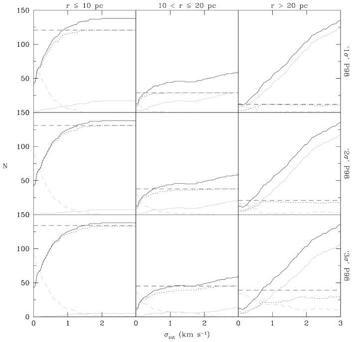
Figure 5: The number of Hyades members found by B99 (this study; solid black), by P98 (dashed black), the intersection B99 I P98 (dotted black), the difference P98 M B99 (dashed grey), and the difference B99 M P98 (solid grey), as function of the (one-dimensional) velocity dispersion $\sigma_{\rm int}$ used in the selection procedure. From the top row down: ‘1$\sigma$’ P98 results (confidence limit $p_{\rm conf}=0.683$), ‘2$\sigma$’ P98 results ($p_{\rm conf}=0.954$), and ‘3$\sigma$’ P98 results ($p_{\rm conf}=0.9973$). From the left column right: stars with $r\leq 10$ pc (‘core’ + ‘corona’), stars with $10<r\leq 20$ pc (‘halo’), and stars with $r>20$ pc (‘moving group population’).

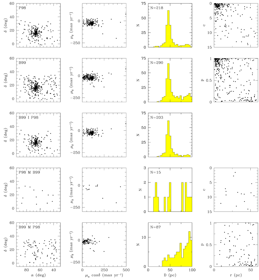
Figure 6: Results of the membership selection of the Hyades by P98 (‘3$\sigma$’ members; top row), B99 (this study; $\sigma_{\rm int}=2.0~{}{\rm km}~{}{\rm s}^{-1}$; second row), B99 and  P98 (B99 I P98; third row), P98 and not  B99 (P98 M B99; fourth row), and B99 and not  P98 (B99 M P98; fifth row). From the left column right: (1) positions on the sky; (2) vector point diagram $(\mu_{\alpha}\cos\delta,\mu_{\delta})$; (3) distance histogram ($D\equiv 1000/\pi$; $D$ in pc, $\pi$ in mas) with number of stars indicated; and (4) membership statistic or probability as function of three-dimensional distance $r$ (pc) from the Hyades cluster centre: $p$ ($0\leq p\leq 1$; eq. 23) versus $r$ for B99 and B99 M P98; the dimensionless quantity $c$, defined by $c\equiv\mn@boldsymbol{z}^{\rm T}{\bf\Sigma}^{-1}\mn@boldsymbol{z}$, where T denotes taking the transpose, $\mn@boldsymbol{z}$ is the difference vector between the observed space velocity of the star and the Hyades centre-of-mass motion, and ${\bf\Sigma}$ is the sum of the two corresponding covariance matrices, for P98 and P98 M B99. In case $\mn@boldsymbol{z}$ is $\nu$-dimensional, $c$ is distributed as $\chi^{2}$ with $\nu$ degrees of freedom: for $\nu=2$ (no radial velocity information), $c=11.83$ corresponds to a confidence limit $p_{\rm conf}=0.9973$ (‘3$\sigma$’), and for $\nu=3$, $c=14.16$ relates to $p_{\rm conf}=0.9973$ (‘3$\sigma$’).

Figure 8(a) in P98 shows the positional distribution of the 218 members. P98 consider four distinct components ($r$ is defined as the three-dimensional distance to the cluster centre): (1) a spherical ‘core’ with a core radius $r_{\rm c}\sim 2.7~{}{\rm pc}$ and half-mass radius $r_{\rm h}\sim 5.7~{}{\rm pc}$; (2) a ‘corona’ extending out to the tidal radius $r_{\rm t}\sim 10~{}{\rm pc}$; (3) a ‘halo’ consisting of stars with $r_{\rm t}\la r\la 2r_{\rm t}$ which are still dynamically bound to the cluster; and (4) a ‘moving group population’ of stars with $r\ga 2r_{\rm t}$ which have similar kinematics as the central parts. The halo and the moving group population are explained by evaporation and diffusion of core and corona members due to the effects of the Galactic tidal field and stellar encounters (§4.2). The core and corona contain 134 stars ($r\leq 10~{}{\rm pc}$), the halo contains 45 stars ($10<r\leq 20~{}{\rm pc}$), and the moving group population contains 39 stars ($r>20~{}{\rm pc}$). Kinematic assignment of membership beyond $\sim$$2r_{\rm t}$ is difficult, and thus less reliable.

Figure 8(b) in P98 shows the velocity distribution of the 218 members. The expected one-dimensional velocity dispersion is 0.2–$0.4~{}{\rm km}~{}{\rm s}^{-1}$, too low to be resolved: the observed velocities are fully consistent with parallel space motions of the members, with a (one-dimensional) velocity dispersion of $\sim$$0.3~{}{\rm km}~{}{\rm s}^{-1}$ due to a combination of internal motions, undetected binaries, and measurement errors.

We apply the convergent point method to the Hyades with $D=45~{}{\rm pc}$, $t_{\rm min}=1.7$, and $\epsilon_{\rm min}=0.954$. Figure 5 shows the results as function of the (one-dimensional) velocity dispersion $\sigma_{\rm int}$ used in the selection. It follows from Figure 5 that: (1) in order to reproduce the P98 results, a non-zero value for $\sigma_{\rm int}$ is required; for $\sigma_{\rm int}\ga 1.5~{}{\rm km}~{}{\rm s}^{-1}$, the numbers of selected stars are comparable to the numbers found by P98; (2) despite the fact that P98 have made use of additional parallax and radial velocity data, the convergent point method is able to retrieve nearly all P98 members in the inner 20 pc of the cluster centre, without introducing many spurious members at the same time. Most of the stars that are not picked up by the convergent point method have a low P98 membership probability (cf. Figure 6). The convergent point method picks up a number of field stars in the outer regions of the cluster, $r\ga 2r_{\rm t}\sim 20~{}{\rm pc}$ (cf. Figure 6). Parallaxes and/or radial velocities are required in order to reject these stars as candidate Hyades members.

Table 2 gives the comparison of this study (B99) and P98 results for $\sigma_{\rm int}=2.0~{}{\rm km}~{}{\rm s}^{-1}$. Figure 6 shows the results of the membership selection and the comparison with the ‘3$\sigma$’ P98 results for $\sigma_{\rm int}=2.0~{}{\rm km}~{}{\rm s}^{-1}$. The convergent point method correctly identifies 203 of the 218 P98 Hyades members. Only 15 P98 Hyades members are not picked up by the convergent point method: 4 of the 15 lie between 9.30 and 16.47 pc from the cluster centre, but have a low membership probability. The same is true for the remaining 11 stars, at $r\geq 26.70~{}{\rm pc}$. Furthermore, only 4 of them have a known radial velocity. Eighty-seven new candidate Hyades members are identified by the convergent point method. Five of them have $r\leq 10~{}{\rm pc}$, but rather low membership probabilities ($p\leq 0.60$). Seven stars have $10<r\leq 20~{}{\rm pc}$. The remaining 75 candidates have $r>20~{}{\rm pc}$, combined with low membership probabilities as well as predominantly small proper motions and parallaxes ($D\ga 50~{}{\rm pc}$), and are distributed uniformly over the sky. This indicates that these stars are most likely field stars, which can be rejected as candidate members using parallax and/or radial velocity information.

We find $X^{2}=245.574$ ($0.853$ per degree of freedom), and $(\alpha_{\rm cp},\delta_{\rm cp})=(95\aas@@fstack{\circ}54\pm 0\aas@@fstack{\circ}43,7\aas@@fstack{\circ}28\pm 0\aas@@fstack{\circ}19)$ with a correlation coefficient $\rho=-0.79$ on the measurement errors (§2.4.3). Projecting the Hyades centre-of-mass motion (table 3 in P98) gives corresponding convergent points of $(\alpha_{\rm cp},\delta_{\rm cp})=(97\aas@@fstack{\circ}91,6\aas@@fstack{\circ}66)$ for the 134 stars with $r\leq 10~{}{\rm pc}$, and $(97\aas@@fstack{\circ}96,6\aas@@fstack{\circ}61)$ for the 179 stars with $r\leq 20~{}{\rm pc}$. When we apply the convergent point method to the 218 P98 members as starting set, we end up with 213 members having $X^{2}=151.712$ ($0.702$ per degree of freedom), $(\alpha_{\rm cp},\delta_{\rm cp})=(97\aas@@fstack{\circ}81\pm 0\aas@@fstack{\circ}52,6\aas@@fstack{\circ}74\pm 0\aas@@fstack{\circ}21)$, and $\rho=-0.84$. The 5 rejected stars have $r>30~{}{\rm pc}$, and 4 of them have no radial velocity information. The different convergent points seem to show a large spread. However, it can be explained fully by the errors: the confidence ellipses are elongated along the great circle which connects the convergent points and the Hyades cluster centre, and the spread in the convergent points is exactly along this great circle. Accordingly, the position of the convergent point is well-defined in the direction perpendicular to this great circle, whereas it can easily shift along the great circle (§3.2.3). This is illustrated by the rejection of the last star in the application of the convergent point method to the 218 P98 members; this step shifts the convergent point from $(\alpha_{\rm cp},\delta_{\rm cp})=(96\aas@@fstack{\circ}70,6\aas@@fstack{\circ}91)$ to $(97\aas@@fstack{\circ}81,6\aas@@fstack{\circ}74)$.

4.2 Hyades supercluster

Figure 7: The 3392 ‘comoving’ Hyades members with $\pi\geq 10$ mas: sky distribution (bottom), parallax distribution (middle), and membership probability distribution (top). The two solid dots in the bottom panel denote the convergent point $(\alpha_{\rm cp},\delta_{\rm cp})=(95\aas@@fstack{\circ}54,7\aas@@fstack{\circ}28)$ and its mirror point $(275\aas@@fstack{\circ}54,-7\aas@@fstack{\circ}28)$.

Although it has often been claimed that the Hyades open cluster is related to a kinematically similar ‘supercluster’ (e.g., Hertzsprung 1909; Eggen 1992; Chereul, Crézé & Bienaymé 1998), these results are not commonly accepted (e.g, Ratnatunga 1988; Skuljan, Cottrell & Hearnshaw 1997). This extended moving group population is generally explained by the evaporation of the Hyades open cluster through (1) relaxation by internal stellar encounters, (2) the Galactic tidal field, and (3) passing interstellar clouds (e.g., Terlevich 1987). Although all these effects are indisputably taking place, it is not to be expected that all escaped members have velocities consistent with the cluster space motion: stars beyond the cluster tidal radius are subject to Galactic tidal forces and to the shearing effect of differential Galactic rotation, and therefore can have systematically distorted motions. A selection criterion different from velocity, e.g., angular momentum, might therefore be more appropriate to identify escaped members (e.g., Innanen, Harris & Webbink 1983; Helmi, Zhao & de Zeeuw 1998; P98). In short, establishing the significance of the reality and the interpretation of superclusters and all-sky stellar streams is an important issue requiring a thorough analysis, beyond the scope of this paper.

Nonetheless, an interesting question is: ‘is there a significant over-abundance of low-$t_{\perp}$ stars for the Hyades convergent point over the whole sky?’ We have applied the convergent point method to the entire Hipparcos Catalogue, subject to the constraint $\pi\geq 10$ mas, to search for ‘comoving’ Hyades members. Out of 22951 targets, we find 3392 such stars, the overwhelming majority of which (94 per cent) has $r>20$ pc. However, their distribution on the sky is completely random, their parallax distribution peaks sharply towards $\pi=10$ mas, and their membership probabilities are distributed uniformly (Figure 7). All these facts are indicative of a non-physical grouping. Indeed, searching for all-sky comoving stars at random cluster velocities (convergent points) yields identical results. An all-sky search using the ACT/TRC catalogues (§5) is practically feasible, but is prone to give even less well-interpretable results because these catalogues (1) each contain 10 times more stars, (2) have proper motion accuracies which are 2–3 times worse than those of Hipparcos, and (3) do not allow the use of parallaxes to make the $\pi\geq 10$ mas cutoff (giving in practice a 50 times larger sample). Obviously, proper motion data alone is insufficient for all-sky moving group analyses; an in-depth investigation of multi-band photometric, spectroscopic, and/or parallax data is required to bring down the number of interlopers significantly.

5 Discussion

The Hipparcos Catalogue (ESA 1997) has opened a new era of stellar kinematical research. The high quality of the data, its homogeneity, and the absence of systematic errors down to the 0.1 mas level, make the Hipparcos proper motions ideally suited for a reassessment of the existence and membership of moving groups in the Solar neighbourhood. As Hipparcos parallaxes do not yield useful constraints on individual tangential space velocities for stars at distances $D\ga 350$–500 pc, a common motion of distant stars is best detected by converging proper motions. The nature of the Hipparcos data, specifically the full covariance matrices provided in the Catalogue and its high quality which sometimes allows to marginally resolve internal motions, combined with increased computer power over the last decades, have necessitated a refurbishment of the convergent point method that was originally developed by Jones in 1971. This method is a maximum likelihood procedure which detects moving groups and selects the corresponding members from a given set of stars with positions and proper motions. The method selects all stars which have proper motions that are consistent with the maximum likelihood convergent point, and assigns individual membership probabilities. The method is known to work well for nearby groups, such as the Hyades, which span a large enough area on the sky so as to allow the proper motions to show their converging pattern (see Cudworth 1998 for a review). The method is biased towards distant stars, as these have generally small proper motions. Therefore, such stars are more likely not to be rejected as members.

Extensive Monte Carlo simulations have been used to fix free parameters. These simulations show that typically $\sim$80 per cent of all cluster members can be retrieved, combined with a contamination of field stars which amounts to $\sim$20 per cent of the total number of (field) stars in the sample (Figure 3). We presented an application of our method to the Hyades with Hipparcos positions and proper motions. The results for stars near the centre of the cluster agree with those of Perryman et al. (1998), who used parallaxes and radial velocities as well to determine membership. An a posteriori inspection of the Hipparcos parallaxes of stars that are selected by the convergent point method but not by Perryman et al. confirms that nearly all of them lie at large distances from the Hyades cluster centre (Figure 6). The majority of these stars have low to medium membership probabilities, consistent with them being field stars.

The abovementioned bias can also be removed by combining the convergent point method with other selection procedures, such as Hoogerwerf & Aguilar’s (1999) ‘Spaghetti method’ which also uses parallax information. De Zeeuw et al. (1999) have done so, and successfully applied the combined procedure to nearby OB associations with Hipparcos data. As expected, the combination of the two methods efficiently eliminates the biases in the individual methods (figure 4 in de Zeeuw et al.). De Zeeuw et al. used a two-step strategy to determine membership, thereby increasing the sensitivity and power of the convergent point method. In the first step, they identified the association using the early-type stars in the Catalogue, with the projected space motion, i.e., convergent point, as result. As the number of field stars among the early-type stars is generally several factors smaller than the numbers assumed in our Monte Carlo simulations (§§3.2.1–3.2.3; Table 1), the convergent point method was able to detect associations out to distances of $\sim$650 pc. In the second step, additional association members of later spectral type were selected from the remaining stars in the Catalogue by assuming the convergent point of the late-type members is equal to that of the early-type members.

Several parametric and non-parametric methods for finding moving groups have recently been developed (Chen et al. 1997; Figueras et al. 1997; Chereul et al. 1998; Hoogerwerf & Aguilar 1999; see also Dehnen 1998). All of them use Hipparcos positions, proper motions, and parallaxes; some of them also require ground-based radial velocities. The latter methods are currently of limited use, as a uniform set of homogeneous radial velocities for the majority of stars in the Hipparcos Catalogue is not available (cf. Udry et al. 1997); the lack of reliable radial velocities for early-type stars is especially severe, so that these methods cannot be used for detection and membership selection of OB associations.

The positions for $\sim$$10^{6}$ stars with $V\la 11$ mag in the Astrographic Catalogue have recently been combined with those in the Tycho Catalogue. The resulting ACT and TRC catalogues list proper motions on the Hipparcos reference frame with accuracies $\sim$3 mas yr^-1 (Urban et al. 1998; Høg et al. 1998). The ACT/TRC catalogues are presently not the ideal catalogues to apply the convergent point method to: in order to bring down the number of interlopers to an acceptable level, a large amount of additional spectroscopic and/or multi-band photometric data is indispensable (§4.2). Future astrometric satellite missions such as GAIA will provide micro-arcsecond astrometry and accurate multi-epoch multi-band photometry down to $V\sim 20$ mag as well as radial velocities accurate to $\sim$3 km s^-1 down to $V\sim 15$ mag for $\sim$$10^{9}$ stars (e.g., Perryman, Lindegren & Turon 1997; Gilmore et al. 1998). Such data will allow the detection of common motion of stars throughout the Galaxy!

Appendix A From $\mn@boldsymbol{(\mu_{\alpha}\cos\delta,\mu_{\delta})}$ to $\mn@boldsymbol{(\mu_{\parallel},\mu_{\perp})}$

For a given convergent point $(\alpha_{\rm cp},\delta_{\rm cp})$, the transformation of $(\mu_{\alpha}\cos\delta\equiv\mu_{\alpha^{\ast}},\mu_{\delta})$ to $(\mu_{\parallel},\mu_{\perp})$ can be carried out using the general recipe outlined in ESA (1997, Vol. 1, §1.5.2). The transformation uses a 4-dimensional vector $\mn@boldsymbol{a}$:

$$\mn@boldsymbol{a}\equiv\left(\begin{array}[]{c}\alpha^{\ast}\\ \delta\\ \mu_{\alpha^{\ast}}\\ \mu_{\delta}\end{array}\right)\stackrel{{\scriptstyle f}}{{\qquad\longrightarrow\qquad}}\left(\begin{array}[]{c}\alpha^{\ast}\\ \delta\\ \mu_{\parallel}\\ \mu_{\perp}\end{array}\right)\equiv\hat{\mn@boldsymbol{a}},$$ (24)

where $\alpha^{\ast}\equiv\alpha\cos\delta$. The covariance matrix of $\hat{\mn@boldsymbol{a}}$, ${\bf C}_{\hat{\mn@boldsymbol{a}}}$, is given by ${\bf C}_{\hat{\mn@boldsymbol{a}}}\equiv{\bf J}_{f}~{}{\bf C}_{\mn@boldsymbol{a}}~{}{\bf J}_{f}^{\rm T}$, where T denotes taking the transpose, ${\bf J}_{f}$ denotes the Jacobian matrix of the transformation $f$, and ${\bf C}_{\mn@boldsymbol{a}}$ is the covariance matrix of $\mn@boldsymbol{a}$. Using eqs (5) and (6), we find that ${\bf J}_{f}\equiv\partial(\alpha^{\ast},\delta,\mu_{\parallel},\mu_{\perp})/\partial(\alpha^{\ast},\delta,\mu_{\alpha^{\ast}},\mu_{\delta})$ is given by:

$$\left(\begin{array}[]{rrrr}1&0&0&0\\ 0&1&0&0\\ -\mu_{\perp}{\rm d}\theta/{\rm d}\alpha^{\ast}&-\mu_{\perp}{\rm d}\theta/{\rm d}\delta&\sin\theta&\cos\theta\\ \mu_{\parallel}{\rm d}\theta/{\rm d}\alpha^{\ast}&\mu_{\parallel}{\rm d}\theta/{\rm d}\delta&-\cos\theta&\sin\theta\end{array}\right),$$ (25)

with

$${{{\rm d}\theta}\over{{\rm d}\alpha^{\ast}}} = {{\sin^{2}\theta}\over{\sin^{2}(\alpha_{\rm cp}-\alpha)}}\left(\tan\delta-\tan\delta_{\rm cp}\cos[\alpha_{\rm cp}-\alpha]\right),$$

$${{{\rm d}\theta}\over{{\rm d}\delta}} = \alpha\sin\delta\left({{{\rm d}\theta}\over{{\rm d}\alpha^{\ast}}}\right)+{{\cos\delta\sin^{2}\theta}\over{\sin(\alpha_{\rm cp}-\alpha)}}$$ (26)

$$\left(\tan\delta\tan\delta_{\rm cp}+\cos[\alpha_{\rm cp}-\alpha]\right).$$

Appendix B Membership probability

The Hipparcos Catalogue provides the five astrometric parameters $\mn@boldsymbol{a}\equiv(\alpha\cos\delta,\delta,\pi,\mu_{\alpha}\cos\delta,\mu_{\delta})^{\rm T}$, where T denotes taking the transpose, together with the 5$\times$5 covariance matrix ${\bf C}$. Appendix A describes how the proper motion components $\mu_{\alpha}\cos\delta$ and $\mu_{\delta}$ can be transformed into $\mu_{\parallel}$ and $\mu_{\perp}$, with the corresponding 2$\times$2 covariance matrix:

$${\bf C}=\left(\begin{array}[]{cc}\sigma_{\parallel}^{2}&\rho\sigma_{\parallel}\sigma_{\perp}\\ \rho\sigma_{\parallel}\sigma_{\perp}&\sigma_{\perp}^{2}\end{array}\right),$$ (27)

where $\rho$ denotes the correlation coefficient between $\mu_{\parallel}$ and $\mu_{\perp}$. We denote the ‘measured’ proper motion components $\mu_{\parallel}$ and $\mu_{\perp}$ by $\overline{\mu_{\parallel}}$ and $\overline{\mu_{\perp}}$. The confidence ellipse with confidence limit $p_{\rm conf}$ in the $\mu_{\parallel}$–$\mu_{\perp}$-plane is defined by the locus of points $(\mu_{\parallel},\mu_{\perp})$ which solve the equation (Press et al. 1992, p. 690–693):

$$\left(\begin{array}[]{cc}\mu_{\parallel}-\overline{\mu_{\parallel}}&\mu_{\perp}-\overline{\mu_{\perp}}\end{array}\right){\bf C}^{-1}\left(\begin{array}[]{c}\mu_{\parallel}-\overline{\mu_{\parallel}}\\ \mu_{\perp}-\overline{\mu_{\perp}}\end{array}\right)=\Delta,$$ (28)

where the parameter $\Delta$ determines the size of the ellipse, and is related to $p_{\rm conf}$ according to:

$$p_{\rm conf}={{1}\over{\Gamma\left(\nu/2\right)}}\int_{0}^{\Delta/2}{\rm d}t\ t^{-1+\nu/2}\exp{(-t)},$$ (29)

with $\nu$ the number of dimensions. After definition of:

$$\widehat{\mu_{\parallel}}\equiv{{\mu_{\parallel}-\overline{\mu_{\parallel}}}\over{\sigma_{\parallel}}},\qquad\mbox{\rm and}\qquad\widehat{\mu_{\perp}}\equiv{{\mu_{\perp}-\overline{\mu_{\perp}}}\over{\sigma_{\perp}}},$$ (30)

eq. (28) can be written as:

$$\widehat{\mu_{\parallel}}^{2}-2\rho\widehat{\mu_{\parallel}}\widehat{\mu_{\perp}}+\widehat{\mu_{\perp}}^{2}=\Delta(1-\rho^{2}),$$ (31)

from which follows that:

$$\widehat{\mu_{\perp}}=\rho\widehat{\mu_{\parallel}}\pm\left[\left(1-\rho^{2}\right)\left(\Delta-\widehat{\mu_{\parallel}}^{2}\right)\right]^{1/2}.$$ (32)

A natural membership probability $p$ can be related to the confidence limit $p_{\rm conf}$ corresponding to the smallest  confidence ellipse that is consistent with $\mu_{\perp}=0$ in the point $(\widehat{\mu_{\parallel}},\widehat{\mu_{\perp}})=({\widehat{\mu_{\parallel}^{\prime}}},{\widehat{\mu_{\perp}^{\prime}}})$. Solving the equations:

$$\left\{\begin{array}[]{rcl}\widehat{\mu_{\perp^{\prime}}}&=&-\overline{\mu_{\perp}}/\sigma_{\perp},\\ \left[{\rm d}\widehat{\mu_{\perp}}/{\rm d}\widehat{\mu_{\parallel}}\right]_{\widehat{\mu_{\parallel}}=\widehat{\mu_{\parallel^{\prime}}}}&=&0,\end{array}\right.$$ (33)

where $\widehat{\mu_{\parallel}^{\prime}}$ and $\widehat{\mu_{\perp}^{\prime}}$ are related through eq. (31), gives the solution $({\widehat{\mu_{\parallel}^{\prime}}},{\widehat{\mu_{\perp}^{\prime}}})=(\pm\rho\sqrt{\Delta},\pm\sqrt{\Delta})$, with the result that:

$$\Delta=\left({{\overline{\mu_{\perp}}}\over{\sigma_{\perp}}}\right)^{2}.$$ (34)

The confidence limit $p_{\rm conf}$ is given by eq. (29) with $\nu=2$: $p_{\rm conf}=1-\exp{(-\textstyle{1\over 2}\displaystyle\Delta)}$. Thus, for a given star with measured proper motion components $\mu_{\parallel}$ and $\mu_{\perp}$ and covariance matrix ${\bf C}$ (eq. 27) the confidence limit $p_{\rm conf}$ of the smallest  confidence ellipse that is consistent with $\mu_{\perp}=0$ is given by $p_{\rm conf}=1-\exp{(-\textstyle{1\over 2}\displaystyle\left[\mu_{\perp}/\sigma_{\perp}\right]^{2})}$. The membership probability $p$ for this star is then given by (cf. eq. 22):

$$p\equiv 1-p_{\rm conf}=\exp{(-\textstyle{1\over 2}\displaystyle\left[{{\mu_{\perp}}\over{\sigma_{\perp}}}\right]^{2})}.$$ (35)

Appendix C Alternative procedure

Instead of using $t_{\perp}$ as membership indicator under the assumption that its distribution is normal with zero mean and unit variance, one can also work in $\phi_{t}$-space, where $\phi_{t}$ is the polar angle in the $t$-plane: $t_{\parallel}\equiv t\sin\phi_{t}$ and $t_{\perp}\equiv t\cos\phi_{t}$. If $t_{\perp}$ and $t_{\parallel}$ are distributed normally (§2.4.2) with unit variance and mean zero and ${\overline{t}_{\parallel}}$, respectively, it follows that:

$$f(\phi_{t},t){\rm d}\phi_{t}{\rm d}t = {{{\rm d}\phi_{t}{\rm d}t}\over{2\pi}}t\exp(-\textstyle{1\over 2}\displaystyle[\{t\cos\phi_{t}\}^{2}+$$ (36)

$$\qquad\qquad\quad+\{t\sin\phi_{t}-{\overline{t}_{\parallel}}\}^{2}],$$

such that:

$$f(\phi_{t}){\rm d}\phi_{t} \equiv \int_{0}^{\infty}{\rm d}tf(\phi_{t},t){\rm d}\phi_{t}={{{\rm d}\phi_{t}}\over{2\sqrt{2\pi}}}\exp{\left(-\textstyle{1\over 2}\displaystyle{\overline{t}_{\parallel}}^{2}\right)}$$ (37)

$$\!\!\!\!\!\!\!\!\!\!\!\left(\sqrt{{{2}\over{\pi}}}+a\exp{\left(\textstyle{1\over 2}\displaystyle a^{2}\right)}\left[1+{\rm erf}\left({{a}\over{\sqrt{2}}}\right)\right]\right),$$

where ${\rm erf}(x)$ is the error function (e.g., Abramowitz & Stegun 1974, eq. 7.1.1) and $a\equiv{\overline{t}_{\parallel}}\sin\phi_{t}$. For ${\overline{t}_{\parallel}}>0$ $(<0)$, the function $f(\phi_{t})$ peaks at $\phi_{t}=\textstyle{\pi\over 2}\displaystyle$ $(\textstyle{3\pi\over 2}\displaystyle)$; the width of the peak increases with decreasing $|{\overline{t}_{\parallel}}|$, i.e., with increasing cluster distance. Thus, an alternative to minimizing $X^{2}$ (eq. 14) is minimizing:

$$X_{\phi_{t}}^{2}\equiv\sum_{j=1}^{N}\left(\phi_{t,j}-\textstyle{\pi\over 2}\displaystyle\right)^{2}\quad{\rm or}\quad\sum_{j=1}^{N}\left(\phi_{t,j}-\textstyle{3\pi\over 2}\displaystyle\right)^{2}.$$ (38)

References

- [1] Abramowitz M., Stegun I.A., 1974, Handbook of mathematical functions, New York: Dover
- [2] Bertiau F.C., 1958, ApJ, 128, 533
- [3] Blaauw A., 1946, PhD Thesis, Groningen Univ. (Publ. Kapteyn Astron. Lab., 52, 1)
- [4] Blaauw A., 1956, ApJ, 123, 408
- [5] Blaauw A., 1964a, ARA&A, 2, 213
- [6] Blaauw A., 1964b, in The Galaxy and the Magellanic clouds, IAU Symp. 20, eds F.J. Kerr & A.W. Rodgers, p. 50
- [7] Blaauw A., 1991, in The physics of star formation and early stellar evolution, eds C.J. Lada & N.D. Kylafis, NATO ASI Ser. C, Vol. 342, p. 125
- [8] Boss L., 1910, Preliminary General Catalogue of 6188 stars for the epoch 1900, Washington, D.C.: Carnegie Institution
- [9] Brown A., 1950, ApJ, 112, 225
- [10] van Bueren H.G., 1952, BAN, 11, 385
- [11] Charlier C.V.L., 1916, Studies in stellar statistics III. The distances and the distribution of the stars of the spectral type B, Lund Medd., Ser. II, 14, 1
- [12] Chen B., Asiain R., Figueras F., Torra J., 1997, A&A, 318, 29
- [13] Chereul E., Crézé M., Bienaymé O., 1999, A&AS, 135, 5
- [14] Cudworth K.M., 1998, in Proper Motions and Galactic Astronomy, ed. R.M. Humphreys, ASP Conf. Ser., Vol. 127, p. 91
- [15] Dehnen W., 1998, AJ, 115, 2384
- [16] Dehnen W., Binney J.J., 1998, MNRAS, 298, 387
- [17] Dravins D., Lindegren L., Madsen S., Holmberg J., 1997, ESA SP–402, p. 733
- [18] Eddington A.S., 1914, Stellar movements and the structure of the universe, London: MacMillan & Co., p. 54
- [19] Eggen O.J., 1992, AJ, 104, 1482
- [20] Elmegreen B.G., Lada C.J., 1977, ApJ, 214, 725
- [21] ESA, 1997, The Hipparcos and Tycho Catalogues, ESA SP–1200
- [22] Feast M., Whitelock P., 1997, MNRAS, 291, 683
- [23] Figueras F., et al., 1997, ESA SP–402, p. 519
- [24] Gilmore G.F., et al., 1998, in Astronomical Interferometry, SPIE Vol. 3350, ed. R.D. Reasenberg, p. 341
- [25] Helmi A., Zhao H.S., de Zeeuw P.T., 1998, in The Galactic halo: bright stars and dark matter; proc. 3rd Stromlo symp., eds B.K. Gibson, T.S. Axelrod & M.E. Putman, ASP Conf. Ser., in press [astro–ph/9811109]
- [26] Hertzsprung E., 1909, ApJ, 30, 135
- [27] Høg E., Kuzmin A., Bastian U., Fabricius C., Kuimov K., Lindegren L., Makarov V.V., Röser S., 1998, A&A, 335, L65
- [28] Hoogerwerf R., Aguilar L.A., 1999, MNRAS, accepted (this issue)
- [29] Innanen K.A., Harris W.E., Webbink R.F., 1983, AJ, 88, 338
- [30] Jones D.H.P., 1971, MNRAS, 152, 231
- [31] Kapteyn J.C., 1914, ApJ, 40, 43
- [32] Kapteyn J.C., 1918, ApJ, 47, p. 104, 146, 255
- [33] Mathieu R.D., 1986, in Highlights of astronomy, Vol. 7, p. 481
- [34] Binney J.J., Merrifield M., 1998, Galactic astronomy, Princeton Univ. Press
- [35] Perryman M.A.C., Lindegren L., Turon C., ESA SP–402, p. 743
- [36] Perryman M.A.C., et al., 1998, A&A, 331, 81 (P98)
- [37] Petrie R.M., 1949a, MNRAS, 109, 693
- [38] Petrie R.M., 1949b, Publ. Dominion Astrophys. Obs., 8, 117
- [39] Press W.H., Teukolsky S.A., Vetterling W.T., Flannery B.P., 1992, Numerical recipes; the art of scientific computing, 2nd ed., Cambridge Univ. Press
- [40] Ratnatunga K.U., 1988, AJ, 95, 1132
- [41] Roman N.G., 1949, ApJ, 110, 205
- [42] Seares F.H., 1944, ApJ, 100, 255
- [43] Seares F.H., 1945, ApJ, 102, 366
- [44] Skuljan J., Cottrell P.L., Hearnshaw J.B., 1997, ESA SP–402, p. 525
- [45] Smart W.M., 1968, Stellar kinematics, London: Longmans, Green and Co., p. 249–253
- [46] Terlevich E., 1987, MNRAS, 224, 193
- [47] Udry S., et al., 1997, ESA SP–402, p. 693
- [48] Urban S.E., Corbin T.E., Wycoff G.L., Martin J.C., Jackson E.S., Zacharias M.I., Hall D.M., 1998, AJ, 115, 1212
- [49] de Zeeuw P.T., Hoogerwerf R., de Bruijne J.H.J., Brown A.G.A., Blaauw A., 1999, AJ, 117, 354