Radio Signatures of H $\scriptstyle\bf I\$at High Redshift: Mapping the End of the “Dark Ages”

Abstract

The emission of 21–cm radiation from a neutral intergalactic medium (IGM) at high redshift is discussed in connection with the thermal and ionization history of the universe. The physical mechanisms that make such radiation detectable against the cosmic microwave background include Ly$\alpha$ coupling of the hydrogen spin temperature to the kinetic temperature of the gas and preheating of the IGM by the first generation of stars and quasars. Three different signatures are investigated in detail: (a) the fluctuations in the redshifted 21–cm emission induced by the gas density inhomogeneities that develop at early times in cold dark matter (CDM) dominated cosmologies; (b) the sharp absorption feature in the radio sky due to the rapid rise of the Ly$\alpha$ continuum background that marks the birth of the first UV sources in the universe; and (c) the 21–cm emission and absorption shells that are generated on several Mpc scales around the first bright quasars. Future radio observations with projected facilities like the Giant Metrewave Radio Telescope and the Square Kilometer Array may shed light on the power spectrum of density fluctuations at $z>5$, and map the end of the “dark ages”, i.e. the transition from the post–recombination universe to one populated with radiation sources.

1 Introduction

The development of structure in the universe was well advanced at high redshifts. Quasars have been detected nearly to $z=5$, and the most distant galaxies to even greater distances (Weymann et al. 1998). The Ly$\alpha\$forest in the spectra of high redshift QSOs shows that the intergalactic medium (IGM) itself developed extensive nonlinear structures by early times. Still unknown, however, is the epoch during which the first generation of stars was formed, and the time scale over which the transition from a neutral universe to one that is almost completely reionized took place. While numerical simulations have shown that the IGM is expected to fragment into structures at early times in cold dark matter (CDM) cosmogonies (Cen et al. 1994; Zhang et al. 1995; Hernquist et al. 1996; Zhang et al. 1998), the same simulations are much less able to predict the efficiency with which the first gravitationally collapsed objects lit up the universe at the end of the “dark age” (Rees 1998). The nature of the first dominant ionizing sources is still unknown, and although IR observations will permit even higher redshift galaxies to be observed, detections become increasingly difficult because of the surface brightness dimming from cosmological expansion.

Madau, Meiksin, & Rees (1997, hereafter MMR) demonstrated that radiation sources prior to the epoch of reionization may be detected indirectly through their impact on the surrounding neutral IGM and the resulting emission or absorption against the cosmic microwave background (CMB) at the frequency corresponding to the redshifted 21–cm line. While its energy density is estimated to be about two orders of magnitude lower than the CMB, the 21–cm spectral signature will display angular structure as well as structure in redshift space due to inhomogeneities in the gas density field (Hogan & Rees 1979; Scott & Rees 1990), hydrogen ionized fraction, and spin temperature (MMR). Because of the smoothness of the CMB sky, fluctuations in the 21–cm radiation will dominate the CMB fluctuations by about 2 orders of magnitude on several arcmin scales. Radio observations at meter wavelengths have therefore the potential to tell us how (as well as when) the primordial gas was reheated and reionized: if the reheating was due to ultraluminous but sparsely distributed sources like QSOs, or by fainter but more uniformly distributed objects like an abundant population of pregalactic stars.

In this paper we discuss possible ways in which the next generation of radio telescopes could provide the first observations of a neutral IGM at a level of a few tenths of $\mu$Jy arcmin^-2. The proposed Square Kilometer Array (SKA) would provide an enhancement of about two orders of magnitude in sensitivity relative to present–day radio telescopes (Taylor & Braun 1999). We discuss the technical requirements necessary to detect the 21–cm signature from the IGM and describe a possible design for a special purpose telescope. We emphasize that within existing technological limits, radio astronomy could effectively open up much of the universe to a direct study of the reheating and reionization epochs.

2 Basic theory

The ground state hyperfine levels of hydrogen will very quickly reach thermal equilibrium with the CMB. In order to detect the IGM in either emission or absorption, it is crucial that an effective mechanism be present to decouple the hydrogen spin states from the CMB. Following MMR, we briefly review below the mechanisms that determine the level populations of the hyperfine state of neutral hydrogen in the intergalactic medium (see also Meiksin 1999).

2.1 Spin temperature

The emission or absorption of 21–cm radiation from a neutral IGM is governed by the hydrogen spin temperature $T_{S}$, defined by

$$\frac{n_{1}}{n_{0}}=3\exp(-T_{*}/T_{S}),$$ (1)

where $n_{0}$ and $n_{1}$ are the singlet and triplet $n=1$ hyperfine levels, $T_{*}\equiv h_{P}\nu_{10}/k_{B}=0.07\,$K, $\nu_{10}$ is the frequency of the 21–cm transition, $h_{P}$ is Planck’s constant, and $k_{B}$ is Boltzmann’s constant. In the presence of only the CMB radiation with $T_{\rm CMB}=2.73\,(1+z)\,$K, the spin states will reach thermal equilibrium with the CMB on a timescale of $T_{*}/(T_{\rm CMB}A_{10})\approx 3\times 10^{5}\,(1+z)^{-1}\,$yr ($A_{10}=2.9\times 10^{-15}\,$s^-1 is the spontaneous decay rate of the hyperfine transition of atomic hydrogen), and intergalactic H $\scriptstyle\rm I\$will produce neither an absorption nor an emission signature. A mechanism is required that decouples $T_{S}$ and $T_{\rm CMB}$, e.g. by coupling the spin temperature instead to the kinetic temperature $T_{K}$ of the gas itself. Two mechanisms are available, collisions between hydrogen atoms (Purcell & Field 1956) and scattering by Ly$\alpha\$photons (Wouthuysen 1952; Field 1958). The collision–induced coupling between the spin and kinetic temperatures is dominated by the spin–exchange process between the colliding hydrogen atoms. The rate, however, is too small for realistic IGM densities at the redshifts of interest, although collisions may be important in dense regions, $\delta\rho/\rho\mathrel{\hbox to0.0pt{\lower 3.0pt\hbox{$\mathchar 536\relax$}\hss}\raise 2.0pt\hbox{$\mathchar 318\relax$}}30[(1+z)/10]^{-2}$ (MMR).

In the low density IGM, the dominant mechanism is the scattering of continuum UV photons redshifted by the Hubble expansion into local Ly$\alpha\$photons. The many scatterings mix the hyperfine levels of neutral hydrogen in its ground state via intermediate transitions to the $2p$ state, the Wouthuysen–Field process. An atom initially in the $n=1$ singlet state absorbs a Ly$\alpha\$photon that puts it in an $n=2$ state, allowing it to return to the triplet $n=1$ state by a spontaneous decay. As the neutral IGM is highly opaque to resonant scattering, the shape of the continuum radiation spectrum near Ly$\alpha\$will follow a Boltzmann distribution with a temperature given by the kinetic temperature of the IGM (Field 1959). In this case the spin temperature of neutral hydrogen is a weighted mean between the matter and CMB temperatures,

$$T_{S}=\frac{T_{\rm CMB}+y_{\alpha}T_{K}}{1+y_{\alpha}},$$ (2)

where

$$y_{\alpha}\equiv\frac{P_{10}T_{*}}{A_{10}T_{K}}$$ (3)

is the Ly$\alpha\$pumping efficiency. Here $P_{10}$ is the indirect de–excitation rate of the triplet $n=1$ state via absorption of a Ly$\alpha\$photon to the $n=2$ level, and $T_{S}\gg T_{*}$ is assumed. If $y_{\alpha}$ is large, $T_{S}\rightarrow T_{K}$, signifying equilibrium with the matter. A consideration of the net transition rates between the various hyperfine $n=1$ and $n=2$ levels above shows that the $1\rightarrow 0$ transition rate via Ly$\alpha\$scattering is related to the total rate $P_{\alpha}$ by $P_{10}=4P_{\alpha}/27$ (Field 1958). This relation and equation (2) are derived in the Appendix. In the limit $T_{K}\gg T_{\rm CMB}$, the fractional deviation in a steady state of the spin temperature from the temperature of the CMB is

$${{T_{S}-T_{\rm CMB}}\over T_{S}}\approx\left(1+{T_{\rm CMB}\over y_{\alpha}T_{K}}\right)^{-1}.$$ (4)

There exists then a critical value of $P_{\alpha}$ which, if greatly exceeded, would drive $T_{S}\rightarrow T_{K}$. This “thermalization” rate is (MMR)

$$P_{\rm th}\equiv{27A_{10}T_{\rm CMB}\over 4T_{*}}\approx(7.6\times 10^{-12}~{}{\rm s}^{-1})~{}\left({1+z\over 10}\right).$$ (5)

2.2 Brightness temperature

Consider a patch of neutral hydrogen with an angular diameter on the sky larger than the beamwidth of the telescope, and a radial velocity width broader than the bandwidth. In an Einstein–de Sitter universe with $H_{0}=100\,h\,\,{\rm km\,s^{-1}\,Mpc^{-1}}$ and baryon density parameter $\Omega_{b}$, the optical depth of the patch at $21(1+z)\,$cm for a spin temperature $T_{S}\neq T_{\rm CMB}$ is

$$\tau(z)=\frac{3}{32\pi}\lambda_{10}^{3}A_{10}\frac{T_{*}}{T_{S}}\frac{n_{\rm HI}(0)}{H_{0}}(1+z)^{1.5}\approx 0.0033\,h^{-1}\left({T_{\rm CMB}\over T_{S}}\right)\left({\Omega_{b}h^{2}\over 0.02}\right)\left({1+z\over 10}\right)^{1/2}.$$ (6)

The optical depth will typically be much less than unity. Since the brightness temperature through the IGM is $T_{b}=T_{\rm CMB}e^{-\tau}+T_{S}(1-e^{-\tau})$, the differential antenna temperature observed at Earth between this region and the CMB will be

$$\delta T_{b}=(1+z)^{-1}(T_{S}-T_{\rm CMB})(1-e^{-\tau})\approx(9.0~{}{\rm mK})h^{-1}\left({\Omega_{b}h^{2}\over 0.02}\right)\left({{1+z}\over 10}\right)^{1/2}\left({T_{S}-T_{\rm CMB}\over T_{S}}\right).$$ (7)

If the intergalactic gas has been significantly preheated, $T_{S}$ will be much larger than $T_{\rm CMB}$, and the IGM will be observed in emission at a level that is independent of the exact value of $T_{S}$. By contrast, when $T_{\rm CMB}\gg T_{S}$ (negligible preheating), the gas will appear in absorption, and $|\delta T_{b}|$ will be a factor $\sim T_{\rm CMB}/T_{S}$ larger than in emission, so that it becomes relatively easier to detect intergalactic H $\scriptstyle\rm I\$(Scott & Rees 1990).

The presence of a sufficient flux of Ly$\alpha\$photons will thus render the neutral IGM “visible.” Without heating sources, the adiabatic expansion of the universe will lower the kinetic temperature of the IGM well below that of the CMB, and the IGM will be detectable through its absorption. If there are sources of radiation that preheat the IGM, it may instead be possible to detect the IGM in emission.

2.3 Preheating

The energetic demand for heating the IGM above the CMB temperature is meager, only $\sim 0.004\,$ eV per particle at $z\sim 10$. Consequently, even relatively inefficient heating mechanisms may be important warming sources well before the IGM has been reionized.  Possible preheating sources are soft X–rays from an early generation of quasars or thermal bremsstrahlung emission produced by the ionized gas in the collapsed halos of young galaxies (MMR). While photons emitted by a quasar just shortward of the photoelectric edge are absorbed at the ionization front, photons of much shorter wavelength will be able to propagate into the neutral IGM much further. Most of the photoelectric heating of the IGM by a QSO is accomplished by soft X–rays. The timescale required for the radiation near the light front to heat the intergalactic gas to a temperature above that of the CMB is typically 10% of the Hubble time. The H $\scriptstyle\rm II\$region produced by a QSO will therefore be preceded by a warming front.

An additional heating source is the Ly$\alpha\$photon scattering itself (MMR). The heating rate by the recoil of scattered Ly$\alpha\$photons is

$$\dot{E}_{\alpha}=\left(\frac{h_{P}\nu_{\alpha}}{m_{\rm H}c^{2}}\right)h_{P}\nu_{\alpha}P_{\alpha},$$ (8)

where $P_{\alpha}$ is the Ly$\alpha\$scattering rate per hydrogen atom, and $m_{\rm H}$ is the mass of a hydrogen atom. In the case of excitation at the thermalization rate $P_{\rm th}$, equation (8) becomes

$$\dot{E}_{\rm th}={27h_{P}^{2}\nu_{\alpha}^{2}A_{10}T_{\rm CMB}\over 4m_{\rm H}c^{2}T_{*}}\approx(315~{}{\rm K\,Gyr}^{-1})\left({{1+z}\over 10}\right).$$ (9)

The characteristic timescale for heating the medium above the CMB temperature via Ly$\alpha\$resonant scattering at this rate is

$$\Delta t={2m_{\rm H}c^{2}\nu_{10}\over 9h_{P}\nu_{\alpha}^{2}}A_{10}^{-1}\approx 10^{8}\,{\rm yr},$$ (10)

about 20% of the Hubble time at $z=8$. This result has an important consequence: if a substantial population of sources of UV radiation turn on quite rapidly at (say) $z\sim 10$, there exists a finite interval of time during which Ly$\alpha\$photons couple the spin temperature to the kinetic temperature of the IGM before heating the gas above the CMB (reionization occurs at even later times). A window is then created in redshift space where a large fraction of intergalactic gas may be observed at $\sim 160\,$MHz in absorption against the CMB. We will show next how this transient phase may imprint a strong signature on the radio sky.

3 Radio signatures

3.1 The “cosmic web” in emission at 21–cm

Numerical $N$–body/hydrodynamics simulations of structure formation within the framework of CDM–dominated cosmologies (Cen et al. 1994; Zhang et al. 1995; Hernquist et al. 1996; Zhang et al. 1998) have recently provided a definite picture for the topology of the IGM at $z\mathrel{\hbox to0.0pt{\lower 3.0pt\hbox{$\mathchar 536\relax$}\hss}\raise 2.0pt\hbox{$\mathchar 316\relax$}}5$, one of an interconnected network of sheets and filaments with virialized systems located at their points of intersection. In between the filaments are underdense regions. This “cosmic web” appears to be a generic feature of CDM (Pogosyan et al. 1998), a pattern imprinted in the matter fluctuations at decoupling and sharpened by gravity. In a UV photoionizing background, modestly overdense filaments ($1<\rho_{b}/{\bar{\rho}_{b}}<5$) will give rise to the Ly$\alpha\$forest seen in the spectra of high redshift quasars. As discussed below, radio observations at meter wavelengths on several arcmin scales may probe the cosmic web at times prior to the epoch of reionization.

Because of the clumpiness of the IGM, the 21–cm optical depth of equation (6) will vary for different lines of sight. To estimate the rms level of brightness temperature fluctuations at $21(1+z)\,$ cm, we shall consider three different cosmological models with parameters suggested by a variety of recent observations: an open model (OCDM, $\Omega_{M}=0.4$, $h=0.65$, $n=1$), a flat model ($\Lambda$CDM, $\Omega_{M}=0.3$, $\Omega_{\Lambda}=0.7$, $h=0.7$, $n=1$), and an Einstein–de Sitter tilted model (tCDM, $\Omega_{M}=1$, $\Omega_{\Lambda}=0$, $h=0.5$, $n=0.8$). In all cases the amplitude of the power spectrum or, equivalently, the value of the rms mass fluctuation in a $8\;h^{-1}$ Mpc sphere, $\sigma_{8}$, has been fixed in order to reproduce the observed abundance of rich galaxy clusters in the local universe (e.g. Eke et al. 1998). The tilted model has been designed to also match COBE measurements of the CMB on large scales. Our choice of an open CDM cosmology (with a normalization which is 2 rms away from the value observed by COBE) is guided by the growing evidence in favour of a low value of $\Omega_{M}$ from cluster studies (e.g. Carlberg et al. 1997). The $\Lambda$–dominated model matches both the cluster constraint on small scales and COBE constraint on large. It is also able to account for most known observational constraints, ranging from globular clusters ages to CMB anisotropies (Ostriker & Steinhardt 1995) to recent analyses of the Type Ia SNe Hubble diagram (Perlmutter et al. 1998; Riess et al. 1998), and just fits within the constraints imposed by gravitational lensing (Kochanek 1996; Cooray et al. 1999). In all cosmologies the baryon density is $\Omega_{b}h^{2}=0.02\,$ (Burles & Tytler 1998). The model parameters are sumarized in Table 1.

Table 1: Cosmological parameters.

Model	$\Omega_{M}$	$\Omega_{\Lambda}$	$h$	$n$	$\sigma_{8}$
tCDM	$1.0$	$0.0$	$0.5$	$0.8$	$0.55$
OCDM	$0.4$	$0.0$	$0.65$	$1.0$	$0.92$
$\Lambda$CDM	$0.3$	$0.7$	$0.7$	$1.0$	$1.1$

As an illustrative example, consider a scenario in which sources of Ly$\alpha\$photons are in sufficient abundance throughout the universe to preheat the IGM to a temperature well above that of the CMB, and to couple the spin temperature to the kinetic temperature of the intergalactic gas everywhere. While the average 21–cm signal is two orders of magnitude lower than that of the CMB (and will be swamped by the much stronger non–thermal backgrounds that dominate the radio sky at meter wavelengths and that must be removed), its fluctuations relative to the mean of the surveyed area – induced in this example by density inhomogeneities only – will greatly exceed those of the CMB. Brightness temperature fluctuations will be present both in frequency and in angle across the sky. At high redshifts, and with a spatial resolution of $\sim 1$ arcmin, a patchwork of radio emission will be produced by regions with overdensities still in the linear regime and by voids. From equations (6) and (7), the rms temperature fluctuation relative to the mean, neglecting angular correlations in the projected IGM density, is

$$\langle\delta T_{b}^{2}\rangle^{1/2}\approx(2.9\,{\rm mK})\,h^{-1}\,\Big{(}{{\Omega_{b}\,h^{2}}\over{0.02}}\Big{)}{(1+z)^{2}\sigma_{\rho}\over[\Omega_{M}(1+z)^{3}+\Omega_{K}(1+z)^{2}+\Omega_{\Lambda}]^{1/2}},$$ (11)

where $\Omega_{K}=1-\Omega_{M}-\Omega_{\Lambda}$ is the curvature contribution to the present density parameter. This corresponds to a rms fluctuation in the observed flux of

$$\langle dI^{2}\rangle^{1/2}=(15\,{\rm\mu Jy~{}arcmin^{-2}})\,h^{-1}\,\Big{(}{{\Omega_{b}h^{2}}\over{0.02}}\Big{)}{\sigma_{\rho}\over[\Omega_{M}(1+z)^{3}+\Omega_{K}(1+z)^{2}+\Omega_{\Lambda}]^{1/2}}.$$ (12)

Here $\sigma_{\rho}$ is the variance of the density field in a volume corresponding to a given bandwidth [$\Delta\nu/\nu=\Delta z/(1+z)$] and angular size $\Delta\theta$. The former corresponds to a comoving length $L\approx(1+z)cH(z)^{-1}\Delta\nu/\nu\,$ Mpc, where $H(z)$ is the Hubble constant and $\nu=1.4/(1+z)$ GHz is the observation frequency, the latter to a comoving radius $R=0.5\Delta\theta(1+z)/d_{a}(z)$, where $d_{a}$ is the angular diameter distance.

On the scales of interest here, one can use the linearly evolved power spectrum $P(k)$ (Bardeen et al. 1986) and a filter function that is a cylinder of radius $R$ and height $L$, to compute the density variance:

$$\sigma_{\rho}={{8D^{2}(z)}\over{\pi^{2}R^{2}L^{2}}}\int^{\infty}_{0}dk\int^{1}_{0}dx{{\sin^{2}(kLx/2)J_{1}(kR\sqrt{1-x^{2}})}\over{x^{2}(1-x^{2})}}(1+fx^{2})^{2}{{P(k)}\over{k^{2}}},$$ (13)

where $J_{1}$ is the Bessel function of order one, $D(z)$ is the linear growth factor (e.g. Peebles 1993), and $f\approx\Omega_{M}^{0.6}$ takes into account the effect of the peculiar velocities in compressing the same emitting volume into a narrower bandwidth (as the Hubble flow is reduced in overdense regions, see Kaiser 1987). In this regime it is also legitimate to assume that the baryons follow the dark matter, since segregation effects are important only on smaller scales. We have verified using $N$–body simulations the validity of the linear approximation and the neglect of angular correlations on scales of $\sim 1$ arcmin.

Figure 1 shows the fluctuation levels at 150 MHz ($z=8.5$) as a function of beam size for the models listed in Table 1. At a fixed bandwidth of 1 MHz, $\langle\delta T_{b}^{2}\rangle^{1/2}$ increases with decreasing angular scale from about 1 to 10 mK as $\sigma_{\rho}$ increases with decreasing linear scale. Since the growth of density fluctuations ceases early on in an open universe (and the power spectrum is normalized to the abundance of clusters today), the signal at a given $\Delta\theta$ is much larger in OCDM than in tCDM at high redshift. In a $\Lambda$CDM universe the level of fluctuations is comparable with OCDM. The range of density fluctuations that would be detectable at the $5\sigma$ level by a projected facility like the SKA is shown in Figure 2, as a function of beam size and frequency bandwidth, and for several assumed integration times. The detection thresholds are scaled according to a theoretical rms continuum noise in a 80 MHz bandwidth at 150 MHz of 64 nJy over an 8 hour integration, allowing for only 21 of the 30 dishes in a compact array configuration (Taylor & Braun 1999),

$$rms=(0.23\,\mu{\rm Jy})\Big{(}{{1\,\rm MHz}\over{\Delta\nu}}\Big{)}^{1/2}\Big{(}{{100\,{\rm hours}}\over{\tau}}\Big{)}^{1/2}.$$ (14)

The central compact array in the ‘straw man’ SKA design proposal has a diameter of $\sim 50$ km in order to achieve 1–10 arcsec resolution. A more appropriate resolution for measuring fluctuations in the IGM intensity is $\sim 1$ arcmin. The compact array would have then to be scaled down to $D_{c}\approx 7\,{\rm km}\,(\Delta\theta/{\rm arcmin})^{-1}$ to be optimized for such an experiment. The dashed lines show curves of constant rms fluctuation of the signal in the corresponding beam. Each angular resolution observation corresponds to a different compact array diameter $D_{c}$ (in other words, the array is being optimally resized to match its resolution to the desired angular scale). Because the received flux is proportional to the solid angle of the beam, the signal decreases with decreasing angular scale until it falls below the detection threshold, indicated by the solid lines. With 100 hours of observation in a tCDM model, 2 $\mu$Jy fluctuations will be detectable only on scales exceeding 3 arcmin. In OCDM, and similarly in $\Lambda$CDM, a signal of $\sim 2\,\mu$Jy may be detected at significantly higher resolution with the same integration time.

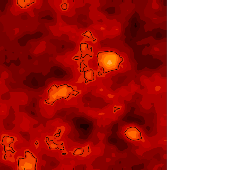
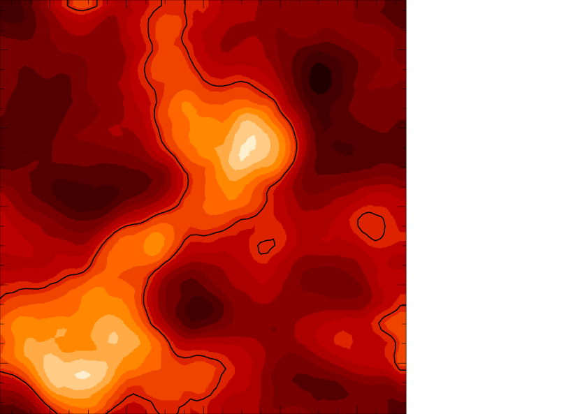
Figure 3: Left: Radio map of redshifted 21–cm emission against the CMB in a tCDM cosmology at $z=8.5$. The linear size of the box is $20h^{-1}$ (comoving) Mpc. The point spread function of the synthesized beam is assumed to be a spherical top–hat with a width of 2 arcmin. The frequency window is 1 MHz around a central frequency of $150$ MHz. The color intensity goes from $1$ to $6\,$ $\mu$Jy per beam. For clarity, the contour levels outline regions with signal greater than $4\,\mu$Jy per beam. Right: Same for OCDM.

Figure 3 show radio maps at $z=8.5$ for tCDM and OCDM, assuming a beamwidth of 2 arcmin and a frequency window of 1 MHz around $150$ MHz. Here a collisionless $N$–body simulation with 64³ particles has been performed with Hydra (Couchman, Thomas, & Pearce 1995). The simulation box size is $20h^{-1}$ comoving Mpc, corresponding to 17 (11) arcmin in tCDM (OCDM). The baryons are assumed to trace the dark matter distribution without any biasing. From a visual inspection of the two simulated images, as well as from Figure 2, it seems possible that observations with a modified (much less spread out) SKA design may be used to reconstruct the matter density field at redshifts between the epoch probed by galaxy surveys and recombination, on scales as small as $0.5-2$ $h^{-1}$ comoving Mpc, i.e. masses in the range between $10^{12}$ and $10^{13}\;h^{-1}M_{\odot}$.

3.2 Observing the epoch of the first stars

In the real universe, the observed radio pattern on the sky depend on a combination of the underlying Gaussian density field and the distribution and luminosities of the sources that cause the preheating and reionization of the IGM. In this and the following sections we shall discuss the detectability of the first radiation sources in the universe through their impact on the surrounding neutral IGM.

In hierarchical clustering theories for the origin of cosmic structure, massive objects grow ‘bottom–up’ – low mass perturbations collapse early, then merge into progressively larger systems. In such a scenario, one naturally expects the high redshift universe to contain small scale substructures, systems with a virial temperature well below $10^{4}\,$K. The resultant virialized systems will remain as neutral gas clouds unless they can cool due to molecular hydrogen, in which case they may form Pop III stars. These stars will produce a background of UV continuum photons near the Ly$\alpha\$frequency which will immediately escape into the IGM, while at the same time ionizing the gas in their vicinity. Ly$\alpha\$photons will propagate into uncollapsed, largely neutral regions of the IGM where the kinetic temperature in the absence of preheating will be

$$T_{K}(z)\approx 26\,{\rm mK}~{}(1+z)^{2}$$ (15)

(Couchman 1985), well below $T_{\rm CMB}$ because of adiabatic cooling during cosmic expansion. If Pop III sources are in sufficient abundance throughout the universe, the Ly$\alpha\$flux will couple the spin temperature to the kinetic temperature, and $T_{S}$ will be pulled below $T_{\rm CMB}$ everywhere. After about $10^{8}$ yr (see eq. 10), the same Ly$\alpha\$photons responsible for the coupling will warm the IGM to a temperature well above that of the CMB. Eventually a sufficient number of photons above 1 Ryd may be able to penetrate all of the surrounding neutral gas in the cloud, reach the external intergalactic gas, and create expanding intergalactic H $\scriptstyle\rm II\$regions.

The crucial assumption we make here is that the Ly$\alpha\$radiation field switches on at a redshift $z>z_{\rm th}$ following the formation of the first stars, and reaches the thermalization value $P_{\rm th}$ at $z_{\rm th}$ on a timescale much shorter than the Hubble time at that epoch. While in hierarchical models of structure formation the spatial number density of halos of a given mass grows initially exponentially (Press & Schechter 1974), the rise time of the UV radiation background will be modulated by gasdynamical processes. In the model of Gnedin & Ostriker (1997), for instance, a Ly$\alpha\$metagalactic flux is rapidly produced in the range $7<z<10$. In this case coupling between $T_{S}$ and $T_{K}\ll T_{\rm CMB}$ is almost instantaneous at $z=z_{\rm th}$, and the IGM is suddenly detectable in absorption. For $z<z_{\rm th}$, Ly$\alpha\$photons begin to heat the IGM and the kinetic temperature increases at the rate

$${dT_{K}\over dz}={{2\mu}\over 3}{\dot{E}_{\rm th}\over k_{B}}{{dt}\over{dz}}+2{{T_{K}}\over{(1+z)}},$$ (16)

until $T_{K}>T_{\rm CMB}$ and the IGM is now detectable in emission. Here, $\mu=16/13$ is the mean molecular weight for a neutral gas with a fractional abundance by mass of hydrogen equal to 0.75. Such a chain of events will leave a strong imprint on the CMB, and mark the epoch of reheating by the first generation of stars. At 150 MHz ($z_{\rm th}=8.5$), the brightness temperature (shown in Figure 4) shows an absorption feature of 40 mK, with a width of about 10 MHz. Such a depression in the CMB is much easier to observe compared with brightness fluctuations, as the isotropic signal may be recorded with a larger beam area. Assuming $\Delta T\simeq 40$ mK as a fiducial estimate, the signal–to–noise ratio for the SKA is

$$\frac{S}{N}\approx 9~{}\Big{(}{{\Delta\nu}\over{1\,\rm MHz}}\Big{)}^{1/2}\Big{(}{\tau\over 100\,{\rm hours}}\Big{)}^{1/2}\,A_{b},$$ (17)

where $\Delta\nu$ is the frequency resolution, $A_{b}$ is the beam area in arcmin², and $\tau$ is the observation time. While the strength of this feature depends mainly on the timescale $t_{\rm th}$ over which the continuum Ly$\alpha$ background field reaches the thermalization value, we have checked that the absorption dip is well above the detection limit for all timescales $t_{\rm th}\mathrel{\hbox to0.0pt{\lower 3.0pt\hbox{$\mathchar 536\relax$}\hss}\raise 2.0pt\hbox{$\mathchar 316\relax$}}0.1t_{H}$, where $t_{H}$ is the then Hubble time. Note that similar sharp signatures in the radio background at meter wavelengths could also be produced at the reionization epoch, as recently discussed by Gnedin & Ostriker (1997) and Shaver et al. (1999).

3.3 Observing the epoch of the first quasars

Very little is actually known observationally about the nature of the first bound objects and the thermal state of the universe at early epochs. If ionizing sources are uniformly distributed, like an abundant population of pregalactic stars, the ionization and thermal state of the IGM will be the same everywhere at any given epoch, with the neutral fraction decreasing rapidly with cosmic time. As discussed above, this may be the case in CDM dominated cosmologies, since bound objects sufficiently massive ($\sim 10^{6}{M_{\odot}}$) to make stars form at high redshift. On the other hand, reionization may also occur in a highly inhomogeneous fashion, as widely separated but very luminous sources of photoionizing radiation such as QSOs, present at the time the IGM is largely neutral, generate expanding H $\scriptstyle\rm II\$regions on Mpc scales: the universe will be divided into an ionized phase whose filling factor increases with time, and an ever shrinking neutral phase. If the ionizing sources are randomly distributed, the H $\scriptstyle\rm II\$regions will be spatially isolated at early epochs.

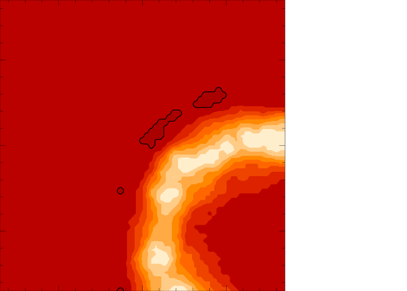
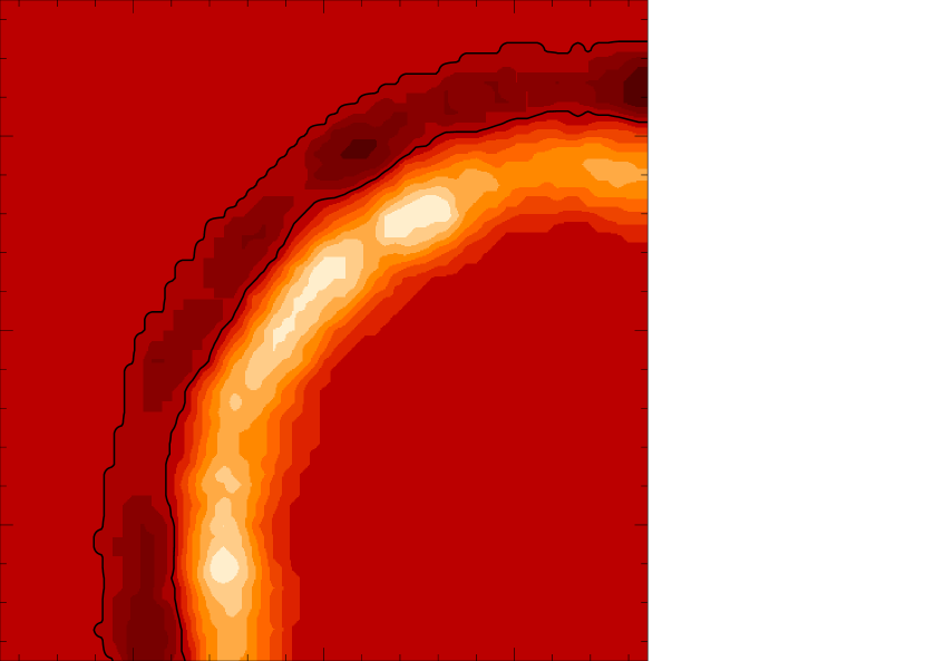
Figure 5: 21–cm emission and absorption against the CMB from the region surrounding a quasar source (lower right corner, in the center of an H $\scriptstyle\rm II\$zone), revealed once the IGM is heated above the CMB by soft X-rays from the quasar. The linear size of the box is of $20h^{-1}$ comoving Mpc (tCDM), the angular resolution is $2$ arcmin, and the bandwidth is 1 MHz. The color levels range from $-3$ $\mu$Jy to $3$ $\mu$Jy per beam. The dark contour demarcates the absorption ring. The quasar turns on at $z=8.5$ with an ionizing photon luminosity of $10^{57}$ photons s^-1, and is observed after $7$ (left) and $10$ (right) Myr. The temperature of the IGM beyond the light radius is assumed to be $T_{K}=26\,{\rm mK}\,(1+z)^{2}\approx 2.3$ K $<T_{\rm CMB}$.

In such a scenario, 21–cm emission on Mpc scales will be produced in the quasar neighborhood as the medium surrounding it is heated by soft X–rays from the QSO itself (MMR). Figure 5 shows the (differential) radio map resulting from a QSO ‘sphere of influence’ soon after it turns on at $z=8.5$ (tCDM). The kinetic temperature profile and radiation field around the quasar were computed including finite light travel time effects and heating by secondary electrons collisionally produced by primary electrons photo–ejected by the soft X–rays (MMR). The specific luminosity of the QSO was taken to be proportional to $\nu^{-1.8}$, normalized to a production rate of H $\scriptstyle\rm I\$ionizing photons of $10^{57}\,{\rm s}^{-1}$. The IGM was assumed uniform with $\Omega_{b}=0.08$ and $H_{0}=50\,{\rm km\,s^{-1}\,Mpc^{-1}}$. The resulting radial temperature profiles were then superimposed on the surrounding density fluctuations as computed using Hydra. The visual effect is due to the convolution of the spin temperature profile with the (linearly) perturbed density field around the quasar. Outside the H $\scriptstyle\rm II\$bubble, there is an inner thin shell of neutral gas where the IGM is heated to $T_{S}=T_{K}>T_{\rm CMB}$ as the hyperfine levels are mixed by Ly$\alpha\$continuum photons from the QSO, and a much larger external shell where $T_{S}=T_{K}<T_{\rm CMB}$ because of adiabatic cooling. At larger distances from the quasar the Ly$\alpha\$coupling strength is weakening as $r^{-2}$, and $T_{S}\rightarrow T_{\rm CMB}$. As the warming front produced by the quasar expands, a growing amount of the surrounding IGM is unveiled both in emission and in absorption. The size and intensity of the detectable 21–cm region depend on the QSO luminosity and age. In the figure the signal ranges from $-3\mu$Jy to $3\mu$Jy per beam.

Note that, although the quasar was placed in a high density region in the corner of the simulation volume, the figure can equally be viewed as the emission due to heating by a beam of soft X–rays from the quasar with an opening angle of $90^{\circ}$. Thus imaging the gas surrounding a quasar in 21–cm emission could provide a direct means of measuring the opening angle of quasar emission.

4 A compact, special purpose, low frequency array

The requirements for observing the epoch of IGM reheating and reionization are a narrow bandwidth ($\Delta\nu\approx$ 1 MHz), to achieve adequate resolution in velocity space at the relevant redshift, and an angular resolution of a few arcminutes, the typical scale of the expected density fluctuations. The straw man proposal for the SKA suggests a large diameter for its central compact array in order to achieve a resolution of $\sim 1-10$ arcsec. While gas density fluctuations would persist to smaller scales in the IGM, Figure 2 shows that the associated signal would drop well below the threshold for a practical detection. For a successful experiment it is necessary to significantly decrease the diameter of the compact array. The current design for the SKA (and the GMRT) has too widely distributed ‘sub–apertures’ for a program oriented toward detecting arcmin scale structures.

An alternative possibility is to build a compact, special purpose radio telescope dedicated to searching for the expected reheating and reionization signals at low frequencies. A single dish with a diameter of 200 m (smaller than Arecibo) would resolve scales of 30 arcminutes, corresponding to $35-50h^{-1}$ comoving Mpc. This is comparable to the largest scale expected for coherent primordial density fluctuations (Pogosyan et al. 1998). Figure 1 shows that the expected brightness temperature fluctuations on this scale will be in excess of 1 mK. The rms brightness temperature is given by the radiometer equation as

$$\Delta T_{B}=(0.33\,{\rm mK})\left(\frac{T_{\rm sys}}{200\,{\rm K}}\right)\left({{1\,\rm MHz}\over{\Delta\nu}}\right)^{1/2}\left({{100\,{\rm hours}}\over{\tau}}\right)^{1/2}$$ (18)

(Burke & Graham–Smith 1997) for a bandwidth $\Delta\nu$ and integration time $\tau$. The system temperature $T_{\rm sys}$ is sky–limited to 200 K in the coldest directions through the Galaxy (Burke & Graham–Smith). If a density fluctuation filled the beam, it would be detectable at the $5\sigma$ level in a 300 hour integration.

Since such structures tend to be filamentary, a more typical covering factor may be $\sim 0.3$, increasing the required integration time by a factor of 10. This may be offset by increasing the bandwidth. The velocity width of a $50h^{-1}$ comoving Mpc filament at $z=8.5$ corresponds to a frequency width at 150 MHz of about 8 MHz. A bandwidth of 5 MHz would then require an integration time of 500 hours. Such a survey operating over several years would enable a substantial range in redshift to be probed.

5 Conclusions

The history of the universe between the epoch of recombination and the birth of bright sources of radiation by $z\mathrel{\hbox to0.0pt{\lower 3.0pt\hbox{$\mathchar 536\relax$}\hss}\raise 2.0pt\hbox{$\mathchar 316\relax$}}5$ is currently shrowded in mystery: the absence of radiation sources leaves this period a “dark age.” Yet spectra of QSOs show not only metal absorption features in their spectra, the signature of ongoing and past star formation, but evidence for non–linear density fluctuations on large scales as well, a “cosmic web” in the form of the Ly$\alpha\$forest.

We have shown that it may be possible to detect both the development of the cosmic web and the epoch of the first radiation sources, whether stars or QSOs, using 21–cm measurements from intergalactic gas. Prior to reionization, the radio signal will display emission and/or absorption structures both in angle across the sky and in redshift. Fluctuations in 21–cm emission will result from non–uniformities in the gas density and from non–uniformities in the distribution of Ly$\alpha\$radiation sources required to decouple the spin temperature from the CMB temperature. With an instrument like the Square Kilometre Array, such fluctuations would be detectable on arminute scales, and so reveal whether the reheating is due to galaxies or QSOs.

Absorption measurements may permit the epoch of the first stellar sources to be determined. The continuum radiation from an early generation of stars, redshifted to Ly$\alpha\$, will couple the spin temperature to the low kinetic temperature of the IGM for a transitory interval before heating the gas above the CMB temperature. The result is a detectable absorption signature against the CMB that would flag the first epoch of massive star formation in the universe. If reheating were due to ultraluminous but sparsely distributed sources (e.g., the first bright QSOs), the resultant patches would have a larger scale than any gravitationally–induced inhomogeneities. Because of the very large scales involved, there is no difficulty in principle in achieving a sufficiently narrow bandwidth and an adequate angular resolution with the SKA or GMRT; the main limitations are the low flux levels and the radio background subtraction. Alternatively, a special purpose telescope dedicated to scanning the sky in frequency along cold lines of sight through the Galaxy may be used to detect the epochs of reheating. Subsequent high resolution measurements with the SKA would provide a means of identifying the nature of the first radiation sources and so shedding new light on the thermal and reionization history of the universe.

Appendix A The Wouthuysen–Field mechanism

Electric dipole radiation (Ly$\alpha\$photons) can induce a spin transition through spin–orbit coupling. The relevant quantum number is the total angular momentum $F=I+J$, where $I$ is the proton spin and $J$ is the total angular momentum of the electron, $J=S+L$. There are six hyperfine states in total that contribute to the Ly$\alpha\$transition. Only four of these, the $n=1$ singlet ${}_{0}S_{1/2}$ and triplet ${}_{1}S_{1/2}$ states (the notation is ${}_{F}L_{J}$), and the two triplet $n=2$ states ${}_{1}P_{1/2}$ and ${}_{1}P_{3/2}$ contribute to the excitation of the 21–cm line by Ly$\alpha\$scattering. The selection rule $\Delta F=0,1$ permits the transitions ${}_{0}S_{1/2}\rightarrow\,_{1}P_{1/2},\,_{1}P_{3/2}$ and ${}_{1}P_{1/2},\,_{1}P_{3/2}\rightarrow\,_{1}S_{1/2}$, and so effectively ${}_{0}S_{1/2}\rightarrow\,_{1}S_{1/2}$ occurs via one of the $n=2$ states. Denoting the occupation number of ${}_{0}S_{1/2}$ by $n_{0}$ and that of ${}_{1}S_{1/2}$ by $n_{1}$, the rate equation for $n_{0}$ is

$$\frac{dn_{0}}{dt}=A_{10}\left(1+\frac{T_{\rm R}}{T_{*}}\right)n_{1}-3A_{10}\frac{T_{\rm R}}{T_{*}}n_{0}+P^{\alpha}_{10}n_{1}-P^{\alpha}_{01}n_{0},$$ (A1)

where the radiation intensity at the 21–cm frequency has been expressed in terms of the antenna temperature $T_{\rm R}$, $I_{10}=2k_{\rm B}T_{\rm R}/\lambda_{10}^{2}$. The ratio $T_{\rm R}/T_{*}$ is the number of 21–cm photons per mode. Here, $P^{\alpha}_{01}$ and $P^{\alpha}_{10}$ are the effective excitation and de–excitation rates due to Ly$\alpha\$scattering. These may be related to the total scattering rate of Ly$\alpha\$photons, $P_{\alpha}$, as shown below.

It is convenient to label the $n=2$ levels as states $2-5$, from lowest energy to highest. Then the external radiation intensity at the frequency $\nu_{ij}$ corresponding to the $i\rightarrow j$ transition may be expressed as the antenna temperature $T_{\rm R}^{ij}$, as above. The temperature corresponding to the energy difference itself, $h\nu_{ij}$, is expressed as $T_{ij}=h\nu_{ij}/k_{\rm B}$. If $A_{ji}$ denotes the spontaneous decay rate for the transition $j\rightarrow i$, then $P^{\alpha}_{01}$ and $P^{\alpha}_{10}$ are given by

$$P^{\alpha}_{01}=3\frac{T^{\rm R}_{03}}{T_{03}}\frac{A_{30}A_{31}}{A_{30}+A_{31}}+3\frac{T^{\rm R}_{04}}{T_{04}}\frac{A_{40}A_{41}}{A_{40}+A_{41}}$$ (A2)

and

$$P^{\alpha}_{10}=\frac{T^{\rm R}_{13}}{T_{13}}\frac{A_{30}A_{31}}{A_{30}+A_{31}}+\frac{T^{\rm R}_{14}}{T_{14}}\frac{A_{40}A_{41}}{A_{40}+A_{41}}.$$ (A3)

The ratios $A_{ji}/A_{\alpha}$, where $A_{\alpha}$ is the total Ly$\alpha\$spontaneous decay rate, may be solved for using a sum rule for the transitions. This states that the sum of all transitions of given $nFJ$ to all the $n^{\prime}J^{\prime}$ levels (summed over $F^{\prime}$ and $m_{F^{\prime}}$) for a given $n^{\prime}J^{\prime}$ is proportional to $2F+1$ (e.g. Bethe & Salpeter 1957). There are four sets of downward transitions to $n^{\prime}=1$, $J^{\prime}=1/2$, corresponding to the decay intensities $I_{51}$, $I_{50}(=0)$, $I_{41}$, $I_{40}$, $I_{31}$, $I_{30}$, $I_{21}$, and $I_{20}(=0)$. These give

$$\frac{I_{51}}{I_{40}+I_{41}}=\frac{5}{3},\quad\frac{I_{40}+I_{41}}{I_{30}+I_{31}}=1,\quad\frac{I_{30}+I_{31}}{I_{21}}=3.$$ (A4)

Similarly, there are four sets of upward transitions to $n^{\prime}=2$, $J^{\prime}=1/2$ or $3/2$, giving the intensities $I_{30}$, $I_{20}(=0)$, $I_{31}$, $I_{21}$, $I_{50}(=0)$, $I_{40}$, $I_{51}$, and $I_{41}$. These ratios are

$$\frac{I_{40}}{I_{41}+I_{51}}=\frac{1}{3},\quad\frac{I_{30}}{I_{21}+I_{31}}=\frac{1}{3}.$$ (A5)

Using $I_{kj}/I_{\alpha}=(g_{k}/g_{\rm tot})(A_{kj}/A_{\alpha})$, where $I_{\alpha}$ is the total Ly$\alpha\$decay intensity summed over all the hyperfine transitions, and $g_{k}=2F+1$ is the statistical weight of level $k$ ($g_{\rm tot}$ is the sum of the weights of the upper levels), gives $A_{20}/A_{\alpha}=A_{50}/A_{\alpha}=0$, $A_{21}/A_{\alpha}=A_{51}/A_{\alpha}=1$, $A_{30}/A_{\alpha}=A_{41}/A_{\alpha}=1/3$, and $A_{31}/A_{\alpha}=A_{40}/A_{\alpha}=2/3$. We then obtain $P_{\alpha}=3A_{\alpha}(T_{\rm R}/T_{\alpha})$ ($T_{\alpha}\equiv h\nu_{\alpha}/k_{\rm B}$), and $P_{10}=(4/27)P_{\alpha}$. Statistical equilibrium for $T_{\rm R}=0$ requires $P_{01}/P_{10}=n_{1}/n_{0}=3\exp(-T_{*}/T_{K})$. Solving the rate equation (A1) for $T_{\rm R}>0$ gives equation (2), where $T_{\rm R}=T_{\rm CMB}$, and where $T_{S}\gg T_{*}$, $T_{K}\gg T_{*}$, and $T_{\rm R}\gg T_{*}$ have been assumed.

Figure 1: Predicted rms brightness temperature fluctuations relative to the average at 150 MHz for the different cosmologies described in the text, as a function of beam size. A neutral medium with spin temperature $T_{S}\gg T_{\rm CMB}$ has been assumed. The bandwidth is 1 MHz (corresponding to a comoving length of 6.5 $h^{-1}$ Mpc for $\Omega_{M}=1$). The data points with error bars show the range of values found in a set of $N$–body simulations for tCDM (squares) and OCDM (triangles).

Figure 2: Detectability of IGM fluctuations in 21–cm flux density per beam (in $\mu$Jy) at 150 MHz ($z=8.5$) by a projected facility like the Square Kilometer Array as a function of beam width and bandwidth. Dashed lines: Size of the rms fluctuations ($0.5\mu{\rm Jy}$, $2\mu{\rm Jy}$, and $5\mu{\rm Jy}$), relative to the mean expected in a beam defined by the angular diameter $\Delta\theta$ and bandwidth $\Delta\nu$. Solid lines: Threshold below which the fluctuations are undetectable ($S/N<5$) with the SKA for integration times of 10, 100, and 500 hours (from top to bottom). Note that this calculation assumes that the array is optimally resized (becoming more compact at coarser angular resolution) in order to match its resolution to the desired angular scale.

Figure 4: Top: Mean $\Delta T=T_{b}-T_{\rm CMB}$ versus frequency for an angular resolution of 1 arcmin and frequency resolution of 1 MHz (solid line), together with the rms fluctuation value (dashed line). The IGM is reheated at $z_{\rm th}=9$. The strong absorption feature in the mean antenna temperature is associated with the fast rise of a Ly$\alpha\$continuum background on a time scale $\approx 10$ Myr (see text), coupling $T_{S}$ with $T_{K}$. Bottom: Corresponding evolution of the kinetic (dashed line), spin (solid line), and CMB temperatures (dotted line).