M4–18: The planetary nebula and its WC10 central star

Abstract

We present a detailed analysis of the planetary nebula M4–18 (G146.7+07.6) and its WC10-type Wolf-Rayet central star, based on high quality optical spectroscopy (WHT/UES, INT/IDS, WIYN/DensPak) and imaging (HST/WFPC2). From a non-LTE model atmosphere analysis of the stellar spectrum, we derive T_eff=31 kK, log($\dot{M}$/$M_{\odot}$ yr^-1)=–6.05, $v_{\infty}$=160 km s^-1 and abundance number ratios of H/He$<$0.5, C/He=0.60 and O/He=0.10. These parameters are remarkably similar to He 2–113 ([WC10]). Assuming an identical stellar mass to that determined by De Marco et al. for He 2–113, we obtain a distance of 6.8 kpc to M4–18 ($E_{\rm B-V}$=0.55 mag from nebular and stellar techniques). This implies that the planetary nebula of M4–18 has a dynamical age of $\sim$3 100 years, in contrast to $\geq$270 years for He 2–113. This is supported by the much higher electron density of the latter. These observations may only be reconciled with evolutionary predictions if [WC]-type stars exhibit a range in stellar masses.

Photo-ionization modelling of M4–18 is carried out using our stellar WR flux distribution, together with blackbody and Kurucz energy distributions obtained from Zanstra analyses. We conclude that the ionizing energy distribution from the Wolf-Rayet model provides the best consistency with the observed nebular properties, although discrepancies remain.

1 Introduction

Low excitation Wolf–Rayet (WR) central stars of planetary nebula (PN; denoted [WR] following van der Hucht et al. 1981) are thought to represent the beginning of hydrogen–deficient central star evolution, just following the ejection of the PN which occurs at the top of the asymptotic giant branch (AGB). However, discrepancies between observed abundances and those predicted by theory, led to the proposal that H-deficient central stars of PN (CSPN) are the result of the re-birth of a white dwarf, after a late helium–shell pulse (Iben et al. 1983). Following this interpretation, the search began for characteristics common to planetary nebulae with WC nuclei, that could be used to distinguish them from those with H-rich central stars, and thus establish that the two classes have followed different evolutions. However, it soon emerged that nebulae associated with [WC] central stars are indistinguishable from those around H-rich CSPN (Gorny & Stasinska 1995) .

To seek a solution to this problem and determine the evolution of WR type nuclei, a flurry of empirical and modelling analyses of WC central stars were carried out by several groups (e.g. Leuenhagen, Hamann & Jeffery 1996, hereafter LHJ). The present study focuses on M4–18 (PN G146.7+07.6, IRAS 04215+6000), a PN with a [WC10] central star (following the classification scheme of Crowther, De Marco & Barlow 1998). One may reasonably ask why is yet another study of a late WC-type CSPN necessary? Recent stellar (LHJ) and nebular (Surendiranath & Rao 1995, hereafter SR) models for M4–18 exist in the literature, together with empirical determinations of its PN properties (e.g. Goodrich & Dahari 1985). The justification is that previous studies considered the star and nebula of M4–18 in isolation, making it impossible to relate nebular and stellar results; additionally a comparison between the nebular properties of M4–18 with other PN associated with spectroscopically similar stars suggests that [WCL] stars can follow different evolutionary paths; this key aspect has never been given due attention. De Marco, Barlow & Storey (1997) and De Marco & Crowther (1998, hereafter DC) carried out a rigorous analysis of the central stars and PNe of the [WC10] central stars CPD–56^∘8032 and He 2–113. We follow these methods for M4–18, so that the relative results can be compared with confidence.

Our analysis of M4–18 also extends the photo-ionization modelling of CPD–56^∘8032 and He 2–113 by DC using flux distributions appropriate for Wolf-Rayet stars. DC identified a major discrepancy between the observed and predicted nebular properties for these PNe; either the lack of heavy element line blanketing in the wind models was to blame, or the geometry and high nebular densities of those PNe meant that they represented poor probes of the Lyman continuum flux of their central stars. As we shall demonstrate, the PN of M4–18, with a significantly lower electron density, provides a more rigorous test of the theoretical flux distribution.

In Section 2 we will describe the observations, while in Section 3 we will discuss basic observational quantities, including reddening. Section 4 discusses the distance towards M4–18, while a quantitative analysis is carried out in Section 5. Archive Hubble Space Telescope (HST) images are presented in Section 6, while we carry out a nebular abundance analysis in Section 7. In Section 8 photo-ionization modelling of the PN is carried out. Finally, we draw our conclusions in Section 9.

2 Observations and data reduction

We have obtained high quality optical spectroscopy of M4–18 using the 4.2 m William Hershell Telescope (WHT), the 2.5 m Isaac Newton Telescope (INT) and the 3.5 m Wisconsin-Indiana-Yale-NOAO telescope (WIYN). Archival International Ultraviolet Explorer (IUE) ultraviolet (UV) spectroscopy and HST optical imaging of M4–18 were obtained from the Uniform Low-Dispersion Archive (Talavera 1988) at the Rutherford Appleton Laboratory, and the HST data archive at the Space Telescope Science Institute, respectively. The HST Wide Field and Planetary Camera 2 (WFPC2) data set is discussed further in Section 6.

2.1 Optical spectroscopy

M4–18 was observed at the INT, using the Intermediate Dispersion Spectrograph (IDS), together with the 235-mm camera and a 1024$\times$1024 pixel Tektronix CCD, between July 17 and 23, 1996. Four settings with the 1200B/Y gratings provided complete wavelength coverage in the range 3800–6800Å, at a spectral resolution of 1.5Å using a 1.5 arcsec slit. Additional observations with the 300V grating and an 8 arcsec slit (including the entire nebula) provided an absolute flux calibration at a spectral resolution of 9.5Å. The data were reduced in a standard manner using the iraf package, with wavelength calibrations achieved using Cu-Ne and Cu-Ar arc lamps and absolute flux calibrated data obtained by comparing our wide slit observations of M4–18 with observations of the Oke (1990) standards B2 iv star BD+33^∘2642 and the Op star BD+28^∘4211.

High spectral resolution ($R\sim$30 000) observations of M4–18 were obtained at the WHT using the Utrecht Echelle Spectrograph (UES) in service mode on November 27, 1996. A 1024$\times$1024 pixel Tektronix CCD provided a complete spectral range of 4200–5850Å; two exposures each of duration 2400 sec achieved a continuum signal–to–noise ratio of 40. The data were reduced in a standard manner using the iraf package, with wavelength calibration achieved relative to a comparison Th-Ar arc. For flux calibration, the Oke (1990) standard G191B2b (DA0) was used. Subsequent data reduction was carried out with the dipso package (Howarth & Murray 1991).

Additional high resolution (R$\sim$19 000) spectroscopy was obtained on November 13, 1998 by D. Sawyer with the WIYN 3.5 m telescope and the DensPak fiber array, in the range 5770-6010Å. Three exposures each lasting 600 s were obtained with a signal–to–noise ratio of 20. The data were reduced with standard iraf routines. Wavelength calibration was with respect to a Th-Ar lamp. These spectra allowed us to measure the radial velocity shifts of the interstellar Na i D lines.

Finally, our high resolution INT and WHT observations were scaled to the continuum level of the wide–slit INT spectra, which were obtained during photometric conditions. By convolving our observed spectrophotometry with suitable synthetic filters (courtesy of J.R. Deacon) we obtained measurements of both wide-band Johnson photometry (V=14.11 and B=14.24 mag) and narrow-band Smith (1968) photometry ($v$=14.14 and $b$=14.16 mag). Our measurements are in reasonable agreement with Shaw & Kaler (1985) who obtained a (nebula corrected) visual brightness of $\sim$14.0 mag.

2.2 Ultraviolet spectroscopy

We utilised four (SWP and LWR/LWP) low resolution IUE large aperture spectroscopic observations of M4–18 obtained between August 1980–August 1991 (LWR8401 was not used because it is affected by a cosmic ray hit at the wavelength of the C ii] line $\lambda$2326, Goodrich & Dahari 1985). Although of poor quality, these provided constraints on the interstellar reddening towards M4–18, and allowed us to obtain estimates of the nebular carbon abundance.

3 Basic observational quantities

3.1 Radial and nebular expansion velocity

The radial velocity was measured from Gaussian fits to the nebular Balmer lines observed in our optical datasets. WHT–UES observations of H$\beta$–$\gamma$ indicated a mean heliocentric radial velocity of –51.6$\pm$1.0 km s^-1 (corresponding to an LSR radial velocity of –50.8$\pm$1.0 km s^-1). These results are supported by our lower resolution INT observations, which indicate a heliocentric radial velocity of –46.1$\pm$5.0 km s^-1.

Figure 1: (Upper panel): observed ultraviolet and optical spectrophotometry of M4–18 (units are erg cm^-2 s^-1) from IUE and INT, together with theoretical energy distributions reddened by E_B-V=0.45 (dashed), 0.55 (dotted), and 0.65 mag (dot-dashed) using a standard Galactic extinction curve (Seaton 1979; Howarth 1983). (Lower panel): As above, except including near and mid-IR photometry from SR and IRAS (filled-in squares), plus a two-component blackbody fit (dotted lines) to the IR excess caused by dust in the PN.

We used the FWHM of nebular profiles (H$\beta$, H$\gamma$ and $\lambda$5755 [N ii]) in our WHT–UES observations (FWHM $\sim$6 km s^-1) to determine the expansion velocity of the PN of M4–18, which was revealed to be $v_{\rm exp}$=19$\pm$0.5 km s^-1. [The value reported on the ESO PN catalogue (Acker et al. 1992) of 12 km s^-1 derives from an average of [O iii] (7.5 km s^-1) and [N ii] (17.0 km s^-1); we note that it is inappropriate to average values obtained from lines belonging to a mixture of ionization stages, since high ionization lines may originate from inner, slower parts of the PN.]

3.2 Interstellar reddening

Reddening determinations towards M4–18 from the literature range from $E_{\rm B-V}$=0.48 (SR) to $E_{\rm B-V}$=0.90 (Goodrich & Dahari 1985). We derive interstellar reddenings using observed Balmer line fluxes, which are listed in Table 1. Our wide-slit INT H$\beta$ nebular flux is in reasonable agreement with the determinations of 1.04$\times$10^-12 erg cm^-2 s^-1 by Goodrich & Dahari (1985), and 1.17$\times$10^-12 erg cm^-2 s^-1 by Carrasco, Serrano & Costero (1983, 1984).

We adopt N_e=10⁴ cm^-3 and T_e=10⁴ K (these are revised slightly in Section 7), and the Galactic extinction law of Howarth (1983) plus hydrogen recombination coefficients from Storey & Hummer (1995). Unfortunately H$\alpha$ is severely blended with [N ii] in our wide slit INT observations, so we have to rely on narrow-slit observations which imply $E_{\rm B-V}$=0.45 mag from H$\alpha$–H$\beta$ (WHT H$\beta$-H$\gamma$ observations imply $E_{\rm B-V}$=0.61).

Table 1: Balmer fluxes (ergs cm^-2 s^-1) measured for the nebular hydrogen lines of M4–18.

Line	WHT–UES	INT–IDS	INT–IDS
	narrow slit	narrow slit	wide slit
H$\alpha$	–	2.69$\times$10-12	–
H$\beta$	6.61$\times$10-13	5.75$\times$10-13	8.95$\times$10-13
H$\gamma$	2.30$\times$10-13	–	–

We can also derive a reddening towards M4–18 following Milne & Aller (1975), using our observed H$\beta$ flux, together with the observed 5GHz flux of 22 mJy from Aaquist & Kwok (1990). This method implies a higher reddening of $E_{\rm B-V}$=0.65 mag.

Therefore, extinctions in the range $E_{\rm B-V}$=0.45–0.65 mag are implied from the nebula, so we can now test which extinction reproduces the observed UV and optical stellar flux distribution, making use of our theoretical energy distribution from Section 5. In Fig. 1, we compare observed UV and optical spectrophotometry of M4–18 with our theoretical model for interstellar extinctions of $E_{\rm B-V}$=0.45, 0.55 and 0.65 mag. We find that 0.55$\pm$0.05 mag, provides the best match to observations. (The only previous reddening determination towards M4–18 from spectrophotometry was by LHJ who obtained $E_{\rm B-V}$=0.70 from a continuum fit to exclusively UV data.) We therefore adopt $E_{\rm B-V}$=0.55 as appropriate to both the nebular and stellar observations of M4–18.

Fig. 1 also includes blackbody fits to the infra-red (IR) excess of M4–18, representing warm dust from its PN, based on near-IR observations from SR, plus colour corrected 12–100$\mu$m photometry from IRAS. We find that a two component blackbody fit is necessary, indicating the presence of hot ($\sim$1800K) and warm ($\sim$300K) dust. DC found somewhat cooler dust properties for CPD–56^∘8032 and He 2–113.

4 The distance to M4–18

Distance estimates to M4–18 range from 1–7 kpc (SR; Cahn, Kaler & Stanghellini 1991). De Marco et al. (1997) obtained estimates of the distances to CPD–56^∘8032 and He 2-113 based on the LSR radial velocities of the interstellar Na i D lines, or following the assumption that the entire bolometric luminosity is re-radiated in the IR by cool circumstellar dust. The electron density of the PN of M4–18 is more than a factor of ten lower than that of CPD–56^∘8032 and He 2-113 (Section 7), with IRAS fluxes about 30 times lower, suggesting that the stellar luminosity is unlikely to be entirely re-radiated in the infrared.

Figure 2: Upper panel: The Na i D lines in the WIYN spectrum of M4–18. The dashed line shows a one-Gaussian fit to the main stellar emission feature. Lower panel: The rectified D2 spectrum in the LSR rest frame, fitted by a three-cloud model (dashed line). D1 is also shown. The vertical line marks the LSR radial velocity of the PN.

In Fig. 2 we present the WIYN/DensPak observations in the spectral region 5880–5900Å, showing the Na i D lines superimposed on a stellar emission blend (C ii M5, C iii M20 and He ii $\lambda$5897, De Marco et al., 1997). To determine the radial velocities of the individual Na i D line components, we used a model that calculates absorption profiles for a variety of interstellar clouds with Gaussian line-of-sight velocity distributions (implemented into the iscalc routine in the dipso package). To rectify the Na i D lines we ‘snipped’ the D2 absorption and neglected the spectrum longward of $\sim$5892Å, thereby approximating the broad emission feature with a single Gaussian (dashed line in the upper panel of Fig. 2).

The three-cloud component fit to the Na i D2 line is presented in Fig. 2 (lower panel), with the corresponding parameters listed in Table 2. Although we were unable to carry out the same procedure for D1, it is clear from Fig. 2 that the positions of the D1 absorption line components match those of the D2 components.

Table 2: Parameters of the three-cloud model shown in Fig.2. The velocity dispersion parameter $b$ is defined in Howarth & Phillips (1986), while $N$ is Na i the column density. The radial velocity (RV) components are in the LSR rest frame, while $D$ is the distance implied by the Brand & Blitz (1993) galactic rotation curve for material near the galactic plane.

Cloud no.	$b$	Log($N$/cm-2)	RV	$D$
	(km s-1)		(km s-1)	(kpc)
1	13.0	13.0	–60.0$\pm$5.0	–
2	20.0	12.8	–37.0$\pm$5.0	$>$1.5
3	12.0	13.6	–10.0$\pm$5.0	$>$1.0

If the –60 km s^-1 radial velocity component is of interstellar origin, the galactic radial velocity map of Brand & Blitz (1993) indicates that M4–18 lies beyond 10 kpc. However, at this distance, M4–18 would lie 1.2 kpc above the galactic plane, where neutral sodium is likely to be scarce (the scale height of neutral hydrogen was determined to be 144$\pm$80 pc by Shull & Van Steenberg 1985), Moreover, the Brand & Blitz (1993) radial velocity curve was obtained from measurements of H ii regions with a scale height of only 67 pc. In the direction of M4–18, it can be considered reasonably accurate up to a distance from the galactic plane of a few times this value ($\approx$200 pc; several measurements of H ii regions at $\sim$400 pc above the galactic plane exist for this line-of-sight). Interstellar material in the direction of M4–18, therefore extends to a distance of $\sim$1.5 kpc, corresponding to a radial velocity of –30 km s^-1. Na i D line components with radial velocity more negative than this value, cannot be interstellar. Considering the uncertainty on the Galactic rotation curve, we identify the observed –37 km s^-1 component to be of interstellar origin. Consequently, Na i D lines simply argue for the distance towards M4-18 being greater than 1.5 kpc.

We attribute the –60 km s^-1 component to nebular material. Although we may expect M4–18 not to have a neutral envelope since it is optically thin (see Section 8), Na i was observed in other PNe by Dinerstein, Sneden & Uglum (1995), some of which are also optically thin. If Na i is present in the PN shell, its expansion velocity can be obtained from the difference between the LSR radial velocity of the PN (–50.8 km s^-1, Section 3) and the radial velocity shift of the Na i D line component at –60 km s^-1. This results in 9 km s^-1, significantly lower than the ionized shell expansion velocity (19 km s^-1). Neutral shells moving considerably slower than the ionized envelopes were detected by Dinerstein et al. (1995) in two other PNe (SwSt 1 and IC3568).

Therefore, we follow the alternative approach of DC for CPD–56^∘8032 and He 2-113 based on assuming a core mass of 0.62 $M_{\odot}$ (obtained by X.-W. Liu [priv. comm.] for five LMC WR CSPN), and applying the helium burning post-AGB evolutionary tracks of Vassiliadis & Wood (1994) to obtain a stellar luminosity of 5250 $L_{\odot}$. Utilising the observed $v$-band magnitude for M4–18 from our spectrophotometry, together with the interstellar extinction of $E_{\rm B-V}$=0.55$\pm$0.05 mag and bolometric correction from our WR model (Section 5.2) we obtain a distance of $\approx$6.8 kpc. This is in excellent agreement with recent statistical distances for M4–18, which range from 6.7–7.1 kpc, as summarised by Zhang (1995) and with the distance implied by the –37 km s^-1 Na i D line component.

Figure 3: Comparison between rectified spectra of M4–18 (WHT–UES, WIYN–DensPak for $\lambda$$>$5845Å) and He 2–113 (DC), demonstrating the striking similarity of their appearances.

Of course, the masses of all WC central stars need not be identical. From Vassiliadis & Wood (1994) and Blöcker (1995), the possible range in luminosity for a CSPN is $\sim$2 500–16 000 L_⊙, corresponding to a possible range in distance of 4.8–12.0 kpc. Consequently, all distances lower than this minimum are excluded. For example, SR adopted a distance of 1 kpc, based on a relationship between the dust temperature and the PN radius (Pottasch et al. 1984). Using our bolometric correction, an unrealistically low stellar luminosity of 110$L_{\odot}$ would be implied for this distance. (Alternatively, an unrealistically high bolometric correction of $-$6 mag would be required assuming the luminosity from SR namely 2 500$L_{\odot}$).

In summary, we adopt a distance of 6.8 kpc to M4–18, assuming a mass and luminosity identical to that obtained by DC for He 2–113. However, although M4–18 and He 2–113 are spectroscopically very similar (Section 5), this assumption could be in error. The existence of massive WC stars and CSPN with very similar spectra, such as He 2–99 ([WC9]) and HD 164270 (WC9) (see Mendez et al. 1991), is a clear indication that spectral similarities do not necessarily indicate similarities in mass. This estimate, on the other hand is in agreement with the limits imposed by stellar evolution.

5 Stellar Analysis

In this Section we will present our stellar spectrum of M4–18, addressing the important question of whether stellar hydrogen is present. We will also obtain stellar parameters using a sophisticated stellar atmosphere model appropriate for Wolf-Rayet stars.

5.1 The stellar spectrum – is hydrogen present?

The stellar spectrum of M4–18 is dominated by emission lines of helium (He i–ii), carbon (C ii–iv) and oxygen (O ii–iii). Our high resolution spectroscopy of M4–18 is presented in Fig. 3 along with a spectrum of the [WC10] central star He 2–113 (from De Marco et al. 1997). It is apparent that their spectral morphologies are remarkably similar, including line widths, suggesting comparable outflow velocities. The nebular lines of the M4–18 PN are much stronger than in He 2–113.

The upper panel of Fig. 4 shows the high resolution rectified UES spectrum, in the rest frame of the H$\beta$ line. This feature appears to broaden at its base; additionally, a blue–shifted absorption (whose minimum intensity is registered at 185 km s^-1 to the blue of the line’s rest wavelength), is apparent from the rectified spectrum in Fig. 4 (upper panel), suggesting that stellar hydrogen is present in the wind. LHJ determined a H/He ratio of $<$10, 0.64 and $<$0.5 by number, for the [WC10] central stars M4–18, He 2–113 and CPD–56^∘8032, respectively. De Marco et al. (1997) noticed the same behaviour in the Balmer lines of CPD–56^∘8032 and He 2–113. However, by comparing these profiles with nebular [O i] lines at 6300 and 6363Å, they demonstrated that the origin of the broad pedestal under the H$\alpha$ and H$\beta$ profiles is more likely to be due to an irregular nebular geometry.

For M4–18, nebular [N ii] $\lambda$5755 and H$\gamma$ are also present in the high resolution UES spectrum, although these are too weak for a comparison to be made. However, we are able to comment on the origin of the P Cygni profile, which cannot be produced by peculiar nebular material. The lower panel of Fig. 4 compares the P Cygni absorption feature in the rest frame of He ii 4859.18Å (transition 8–4), together with the adjacent Pickering members $\lambda$4541.46 (9–4) and $\lambda$5411.37 (7–4). We find that He ii is responsible for this feature.

To summarise, we suspect that H$\beta$ emission wings are solely due to high velocity components in the nebular spectrum, as is the case for the other two [WC10] central stars He 2–113 and CPD–56^∘8032. (De Marco et al. 1997; Sahai, Wotten & Clegg 1993). To verify this, one would need to observe other nebular lines at high spectral resolution.

Figure 4: (upper panel) Base of the rectified H$\beta$ profile in the WHT–UES dataset of M4–18, revealing the presence of (i) broad line wings and (ii) a P Cygni component; (lower panel) Comparison of rectified He ii Pickering series profiles, indicating that the H$\beta$ P Cygni component is due to He ii $\lambda$4859 (8–4).

5.2 Spectroscopic analysis

Hillier (1987, 1990) theoretical model atmospheres are used in our spectroscopic analysis. These calculations employ an iterative technique to solve the transfer equation in the co-moving frame subject to statistical and radiative equilibrium in an expanding, spherically-symmetric, homogeneous and steady-state atmosphere. The stellar radius ($R_{\ast}$) is defined as the inner boundary of the model atmosphere and is located at a Rosseland optical depth of 20. The temperature stratification is determined from the assumption of radiative equilibrium with the temperature parameter ($T_{\ast}$) defined by the usual Stefan-Boltzmann relation. Similarly, the effective temperature ($T_{\rm eff}$) relates to the radius ($R_{\rm 2/3}$) at which the Rosseland optical depth equals 2/3. The spectral synthesis proceeds by fitting line profiles to observed diagnostic He i-ii, C ii-iv, O ii-iii lines, together with the absolute visual magnitude. In the absence of high resolution ultraviolet observations we measured a stellar wind terminal velocity from optical He i P Cygni profiles, resulting in 160$\pm$15 km s^-1.

Table 3: Derived stellar parameters of M4–18, including a comparison with Leuenhagen et al. (1996, LHJ) scaled to our assumed luminosity, and demonstrating its very close similarity with He 2–113 (from De Marco & Crowther 1998, DC). We include the predicted H i and He i continuum ionizing fluxes ($Q_{0}$, $Q_{1}$).

Star	Study	V	$d$	$E_{\rm B-V}$	$T_{\ast}$	$R_{\ast}$	log $L_{\ast}$	log $\dot{M}$	$v_{\infty}$	H/He	C/He	O/He	log $Q_{0}$	log $Q_{1}$	$M_{\rm V}$
		mag	kpc	mag	kK	$R_{\odot}$	$L_{\odot}$	$M_{\odot}$ yr-1	km s-1				s-1	s-1	mag
M4–18	This work	14.1	6.8	0.55	31	2.4	3.72	$-$6.0	160	$<$0.5	0.60	0.10	47.2	36.7	$-$1.8
	LHJ	13.3	3.5	0.70	31	2.3	3.67	$-$6.0	350	$<$10	0.40	0.05			$-$1.6
He 2–113	DC	11.9	1.2	1.00	31	2.5	3.72	$-$6.1	160	0.0	0.55	0.10	47.2	36.7	$-$1.8

Figure 5: A comparison between selected theoretical profiles for M4–18 (dotted lines) with WHT–UES observations (solid lines). Other profile fits are comparable to those shown for He 2–113 in DC.

Fig. 5 presents a comparison of selected observed (WHT–UES) line profiles (solid) with our synthetic spectra (dotted) for M4–18. Overall, the quality of these and other profile fits, covering a wide range in excitation and ionization, is comparable with that achieved for other [WC10] stars by DC, where a more comprehensive explanation of the successes and failures of the model is presented. Overall the fits successfully reproduce the strength and shape of many optical emission line profiles. In particular the helium spectrum is well fitted, although it is clear from the poor fit to the width of He ii $\lambda$4686 (Fig. 5 - top right panel) that the adopted $\beta$=1 velocity law is not ideal for this star. P Cygni absorption components are poorly predicted (e.g. C iv $\lambda\lambda$5801–12), further supporting an inadequate velocity structure.

Table 3 presents a summary of our derived stellar parameters. Overall, as reflected in their spectra, the stellar properties and chemistries derived for M4–18 and He 2–113 are almost identical, except for a marginally stronger stellar wind and higher carbon content in the former. For reasons discussed by DC we consider that derived parameters are not critically dependent on our neglect of heavy element line blanketing. Although we favour a non-stellar origin for the pedestal at the base of the H$\beta$ line, we have determined a strict upper limit for the stellar hydrogen abundance from fitting the wings of the broad H$\beta$ feature, yielding H/He$<$0.5, by number. Our upper limit, imposes a tighter constraint on the hydrogen abundance than the analysis of LHJ; this is solely due to the higher spectral resolution of our observations (10 km s^-1 versus $\sim$150 km s^-1).

LHJ included M4–18 in their quantitative study of [WCL] CSPNe. Although their study used an independent code, the same assumptions of spherical symmetry and homogeneity were made. Table 3 also compares our derived stellar parameters with those from LHJ. Overall agreement is very good, although LHJ adopt a higher terminal velocity, again due to the lower resolution of their data set. LHJ derive somewhat lower carbon and oxygen contents for M4–18.

Note that the distance to M4–18 adopted by LHJ is inconsistent with our value, despite deriving an almost identical stellar luminosity. This is because LHJ obtained an extinction of $E_{\rm B-V}$=0.7 mag on the basis of a spectral fit to exclusively UV data, inconsistent with our stellar and nebular data sets. Their distance estimate of 3.5 kpc (following Cudworth 1974) then led to a visual continuum magnitude of $v$=13.3 mag, which our spectrophotometry does not support (Section 3).

6 The M4–18 nebula

We now discuss the PN associated with M4–18, including archive HST/WFPC2 narrow-H$\alpha$ (F656N) images, obtained on April 18, 1996 by R. Sahai. From previous ground based observations, the PN of M4–18 is known to be extremely small. Radii from optical, mid-IR and radio data sets suggest $\approx$2^′′ (Shaw 1985; Zijlstra, Pottasch & Bignell 1989). Although the HST/WFPC2 H$\alpha$ image has recently been presented by Sahai & Trauger (1998), we show it in Fig. 6 in connection with further measurements of its size which are relevant to our analysis. We will abstain however from discussing its morphology, which is described in detail by Sahai & Trauger (1998). Fig. 6 shows the nebula both as a grey-scale and a contour map, indicating a clear elongated ring which peaks in intensity at a semi-major axis of 1.28^′′ (PA=0) and a semi-minor axis of 0.8^′′ (PA=90). The ring is embedded in a larger, less eccentric shell. From an azimuthal average of the PN, we determine a mean radius of $1.85^{\prime\prime}\pm 0.10^{\prime\prime}$.

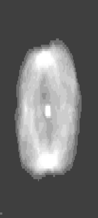
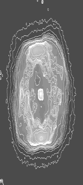
Figure 6: The HST/WFPC2 narrow-band H$\alpha$ (F656N) image of M4–18, shown as a grey–scale plot (left) and a contour plot (right). We present the combined data sets (u35t2401, u35t2402) of R. Sahai, each of 350 sec duration. North is towards the top, east to the left while the field of view is 4.5$\times$4.5^′′.

At a distance of 6.8 kpc, the radius of M4–18 corresponds to a physical radius of 0.06 pc (10⁴ AU). Using the observed nebular expansion velocity we obtain a dynamical age of $\tau_{\rm dyn}$$\sim$3 000 years. Note that this dynamical age should be reasonable since as we will later show, the PN is optically thin (Section 8).

7 Nebular Abundance Analysis

Spectroscopy of the M4–18 PN has previously been carried out by Sabbadin (1980), Goodrich & Dahari (1985) and SR. The latter groups combined low resolution optical and UV spectroscopy to determine PN physical conditions and abundances, while SR also applied their own nebular modelling code. We shall now re-derive the electron density and temperature for the PN of M4–18, together with elemental abundances.

7.1 Nebular line fluxes

Our analysis of the PN associated with M4–18 is based on our INT spectrum, in which stellar and nebular features are blended. (Since the nebular diameter is $\sim$3.7^′′, ground-based long-slit spectroscopy do not allow off-star nebular extraction). We present observed and de-reddened line fluxes in Table 4.

The [O ii] doublet at 3726 and 3729Å may be contaminated by a component of the stellar O ii M2 triplet $\lambda$3727.3. This was judged to be negligible since the un-blended components of this triplet (at 3712.7 and 3749.5Å) were weak. However, this doublet was located close to the end of our spectral range, where the sensitivity of the instrument drops sharply. We therefore assign a 30% error to our measurements. Inspection of our UES data set reveals that both the [Oiii] lines at 5007 and 4959Å are present, though extremely weak.

Following the approach discussed in De Marco et al. (1997) for the C iii] $\lambda$1909 line, we consider this to be entirely of stellar origin. Instead, we rely on C ii] $\lambda$2326 for the determination of the nebular carbon abundance. Its observed equivalent width is 15$\pm$4Å from our dereddened IUE spectrum, of which $\sim$4Å is of stellar origin according to our stellar analysis (Section 5). Since the continuum flux at 2326Å is in good agreement with our reddened theoretical model distribution (Fig. 1), we are able to obtain a nebular $\lambda$2326 flux of 5.34$\times$10^-12 erg cm^-2 s^-1.

For sulphur, only [S ii] $\lambda$$\lambda$6713,31 were available. The [S iii] $\lambda$3722 line is extremely weak (and blended with [O ii] $\lambda$$\lambda$3726,29), while the $\lambda$$\lambda$9069,9532 lines were outside our observed spectral range. SR derived the abundance of S²⁺/H⁺, although they derived fluxes for $\lambda$$\lambda$9069,9532. from indirect techniques. Finally, for nitrogen we used lines at 5755 and 6548Å, excluding [N ii] $\lambda$6584 which is blended with the stellar C ii line at 6578Å.

Table 4: Observed (F) and dereddened (I; $E_{B-V}$=0.55 mag) nebular line intensities for M4–18 from our INT/IDS spectrum ($\ast$: WHT/UES). The dereddened H$\beta$ flux is 3.62$\times$10^-12 erg cm^-2 s^-1. Errors are indicated.

Ion	$\lambda$	F	100$\times$I	Errors
	(Å)	(ergs cm-2 s-1)	/I(H$\beta$)	%
$[$O ii]	3726.0	5.69$\times$10-13	158	30
$[$O ii]	3728.8	3.01$\times$10-13	83.7	30
H$\beta$	4861.3	5.75$\times$10-13	100	10
$[$O iii]	5006.8∗	$\leq$3.6$\times$10-15	0.06	50
$[$N ii]	5754.6	1.11$\times$10-14	1.35	10
$[$O i]	6300.3	2.15$\times$10-14	2.2	10
$[$O i]	6363.8	9.73$\times$10-15	1.0	10
$[$N ii]	6548.0	4.44$\times$10-13	43.1	10
H$\alpha$	6562.8	2.69$\times$10-12	260	10
$[$N ii]	6583.4	1.54$\times$10-12	147	20
$[$S ii]	6716.5	7.19$\times$10-14	6.7	10
$[$S ii]	6730.8	1.41$\times$10-13	13.0	20

7.2 Nebular temperatures, densities and abundances

Figure 7: Nebular Diagnostic diagram for M4–18.

We can now proceed to obtaining estimates of the nebular conditions and chemistry. From the usual diagnostic diagram relating H$\alpha$/[S ii] to [S ii] $\lambda$6717/$\lambda$6731 (see Sabbadin, Minello & Bianchini 1977) we find that M4–18 falls in the photo-ionization dominated region, rather than being ionized by shock waves. Therefore the usual nebular diagnostic techniques may be applied here.

We have constructed a nebular diagnostic diagram for M4–18 using [N ii], [S ii] and [O ii] line ratios. These are generated using the ratio program, written by I.D. Howarth and S. Adams which solves the equations of statistical equilibrium allowing a determination of $N_{e}$ as a function of $T_{e}$ for each ratio. From Fig. 7 we determine $N_{e}$ =10^3.7±0.2 cm^-3 and $T_{e}$=8 200$\pm$200 K for M4–18. The electron density is adopted as a compromise between the [O ii] and [S ii] doublets. Our results are in reasonable agreement with Sabbadin (1980) and SR , though Goodrich & Dahari (1985) derived a somewhat lower electron temperature ($T_{e}$=5600$\pm$1600 K, $N_{e}$=10^4.0±0.1 cm^-3).

Table 5: Nebular abundances for M4–18 (on the usual scale where $\log$N(H)=12.0). The C/O number ratio is on a linear scale. The [Ne ii] line flux is taken from Aitken & Roche (1982).

Ratio	$\log$(X/H)+12.0	Diagnostic Lines
C	9.08$\pm$0.03	C ii] $\lambda$2326
N	7.60$\pm$0.04	[N ii] $\lambda$5755,$\lambda$6548
O	8.62$\pm$0.01	[O ii] $\lambda\lambda$3726,29
Ne	6.73$\pm$0.05	[Ne ii] 12.8 $\mu$m
S	6.16$\pm$0.06	[S ii] $\lambda\lambda$6713,31
C/O	2.9$\pm$0.6

We now utilise our derived nebular parameters to obtain estimates of elemental abundances, which are listed in Table 5. For oxygen, nitrogen and carbon we believe the abundances derived from the singly ionized ions to be representative of the whole ionized populations since [O iii] $\lambda$5007 and C iii] $\lambda$1909 are extremely weak or absent. In the case of oxygen, from the upper limit of $\lambda$5007, we derive O²⁺/H⁺$<$4.4$\times$10^-7, corresponding to O²⁺/O⁺$<$1.0$\times$10^-3.

Equally for sulphur, S⁺/H⁺ should be representative of S/H since SR obtained S²⁺/S⁺$\sim$0.1. Our C/O ratio is much lower than found by De Marco et al. (1997) for CPD–56^∘8032 and He 2–113, which suggests that the carbon abundance in the PNe of WC central stars is not always higher than average.

Overall, agreement with the abundances obtained by SR is good, except for oxygen (they derived log(O/H)+12=8.1) since their de-reddened [O ii] $\lambda$$\lambda$3727,29 flux was almost 10 times lower than our measurement. Abundances derived by Goodrich & Dahari (1985) are also in reasonable agreement once the different reddening and electron properties are taken into account.

8 Nebular Modelling

In this Section we derive Zanstra temperatures for M4–18 using blackbody and Kurucz (1991) model atmosphere flux distributions, which are compared to WR flux distribution resulting from the analysis of the CSPN (Section 5). The nebular radial density profile is derived from the HST H$\alpha$ image surface brightness distribution following the formalism of Harrington & Feibelman (1983). We will finally carry out photo-ionization modelling of the PN of M4–18 using all available atmosphere flux distributions and we will finally compare the modeled parameters with those derived empirically in Section 8.

8.1 Zanstra temperatures

We derive a flux of hydrogen–ionizing photons corresponding to log $Q_{0}$=46.81 s^-1 from our H$\beta$ flux (Table 1), de-reddened by $E_{\rm B-V}$=0.55 at a distance of 6.8 kpc. We derive a blackbody H i Zanstra temperature of 29 500$\pm$500 K, while Kurucz ATLAS9 (Kurucz 1991) model atmospheres yield an effective temperature of 33 000$\pm$500 K, using log $g$=4.0 models (the minimum gravity tabulated at the required effective temperature). The inferred bolometric luminosities are 4000 $L_{\odot}$ and 5600 $L_{\odot}$, respectively. For comparison, Goodrich & Dahari (1985) derived a temperature of 22 000 K using the Stoy (1933) energy–balance method. SR derived a blackbody H i Zanstra temperature of 26 000K. (They also fitted a blackbody to the optical and UV energy distribution implying 23 000 K.)

Our WR stellar model for M4–18 predicts log $Q_{0}$=47.23 s^-1. This is 2.6 times greater than that inferred from the nebular H$\beta$ flux. In contrast, DC showed how the WR model atmosphere ionizing flux of He 2–113 was 85 times larger than that predicted by H$\beta$, suggesting that for high density PN, gas–dust competition might play a role. Our results for M4–18 confirm their suspicion.

8.2 Nebular surface brightness and density distributions

We have obtained the radial density distribution for M4–18, necessary for photo-ionization modelling, from the archival HST/WFPC2 image (Section 6). For this PN the contribution from nebular continuum emission is negligible.

The azimuthally averaged surface brightness distribution in the H$\alpha$ image was derived using an algorithm implementation in the surfphot package of midas. The centre of the image was chosen to coincide with the position of the central star. The integrated flux within a radius $r$ was then determined. The central star was contained within a radius of 5 pixels and the contribution of its continuum flux was subtracted from the nebular flux. The nebular flux, integrated over the entire PN, was then normalised to the de-reddened H$\beta$ flux, differentiated with respect to $r$ and divided by 2$\pi r$ to obtain the required azimuthally averaged H$\beta$ surface brightness distribution. The result is plotted in Fig. 8 (solid line).

Figure 8: H$\beta$ surface brightness profile (in units of erg cm^-2 s^-1 arcsec^-2) derived from the HST H$\alpha$ image of M4–18 from an azimuthal average centred on the star (solid line; the central star’s continuum is responsible for the intensity peaking near the centre of the nebula). The dashed line is the intrinsic surface brightness distribution predicted by our photo-ionization model.

For optically thin PNe, the formalism of Harrington & Feibelman (1983) allows one to derive a density distribution from a surface brightness distribution (see Liu et al. 1995 for an implementation of this method). Photo-ionization models based on density distributions derived with this formalism, however, tend to give an average density which is too low to reproduce density-sensitive line ratios such as the [O ii] $\lambda$3726/$\lambda$3729 ratio. This deficiency is overcome by introducing a filling factor, $\epsilon$, such that within any small region of material a fraction $\epsilon$ is filled with gas, while the complementary fraction (1–$\epsilon$) is empty. In our case all density sensitive line ratios were well reproduced with a filling factor of unity (i.e. a completely filled nebula).

The density distribution which reproduces the H$\beta$ surface brightness distribution, absolute H$\beta$ value and density sensitive line ratios is shown in Fig. 9 (upper panel). To reproduce the surface brightness shown in Fig. 8 we used $N=12$ and $K=1$ in equation A2 of Harrington & Feibelman (1983). The upper panel of Fig.9 shows that M4–18 has a central cavity surrounded by a thick shell whose density declines fairly symmetrically as the radius increases.

Figure 9: (Upper panel): Electron density distribution for M4–18 obtained from our analysis of the HST/WFPC2 image; (Lower panel): Electron temperature resulting from our photo-ionization modelling with the WR flux distribution (assuming a distance of 6.8kpc).

8.3 The photo-ionization modelling

The photo-ionization code used to model M4–18 (Harrington et al. 1982) assumes that the nebula can be represented by a hollow, spherical shell which is ionized and heated solely by the radiation of the central star. This shell is sampled by a network of grid points at each of which the density is supplied. We used 60 grid points and the electron density derived from the H$\beta$ surface brightness (Section 8.2).

Once a distance is adopted, and the de-reddened V magnitude of the central star established, the effective temperature of the central star (from the WR stellar analyis or derived by a Zanstra analysis as described in Section 8.1) determines all the other stellar parameters. These parameters are listed in the first three rows of Table 6. The inner nebular radius was fixed at the value derived from the HST/WFPC2 observations, scaled to the adopted distance. Elemental abundances are initially set at empirical values, and later adjusted to fit the observed line fluxes if necessary.

Final photo-ionization models for each flux distribution are compared to observation in Table 6. Overall, very good agreement is reached between observations and model calculations for all diagnostic line ratios (O ii, N ii and S ii) as well as absolute line fluxes. This is an indication of the success of our density distribution, recalling the discrepancy between different diagnostics in Fig. 7.

It is apparent that the WR and Kurucz (1991) stellar flux distributions perform better than the blackbody. Overall, the WR stellar atmosphere is most appropriate to reproduce the line intensities, in spite of the other distributions resulting from Zanstra nebular analyses. In Fig. 9, we present the predicted electron temperature as a function of radius for our WR model. Hydrogen is completely ionized throughout, as is appropriate for an optically thin PN, with a predicted nebular mass of 0.08$M_{\odot}$.

A major failure of each model flux distribution is the overestimate of the sulphur ionization balance, and consequent underestimate of the [S ii] 6717,31Å line strengths. (The ratio S²⁺/S⁺ was estimated to be 0.1 by SR, although a value of $<$1 is probably more secure.) The poor reproduction of the sulfur ionization balance can be appreciated by inspecting the shape of the ionizing flux distributions in Fig. 10. Metal line blanketing in our WR model atmospheres may help to solve the sulphur problem by reducing the hard UV flux (for the effect of blanketing in late-type WR stars see Crowther, Bohannan & Pasquali 1998).

Figure 10: Comparison of Lyman ionizing flux distribution obtained from our stellar analysis of M4–18 (Wolf-Rayet, solid), with black-body (dashed) and Kurucz (1991, dotted) distributions obtained from our nebular Zanstra analysis. Clearly the WR distribution differs dramatically from the other distributions shortward of the He i edge at $\lambda$504, especially at the O ii edge at $\lambda$353.

In the case of the oxygen ionization balance, only the WR model predicts the appropriate ratio, with Kurucz (1991) and blackbody atmospheres overestimating the strength of [O iii] $\lambda$5007. This is illustrated in Fig. 10 where only the WR energy distribution has negligible zero flux below the He i edge at $\lambda$504.

Table 6: Comparison of results from photo-ionization models for M4–18 with observations (I(H$\beta$)=100), using WR non–LTE, blackbody and Kurucz (1991) plain–parallel energy distributions. Elemental abundances are by number. Filling factors of $\epsilon$=1 are assumed throughout.

Parameter	Empirical	WR	Blackbody	Kurucz
$T_{\em eff}$(kK)	–	31.0	29.5	33.0
log($L_{\ast}/L_{\odot})$	–	3.72	3.60	3.75
log $Q_{0}$(s-1)	46.81	47.23	46.81	46.81
$N_{e}(r)$(cm-3)	See Figure 9 (upper panel)
He/H	–	0.1	0.1	0.1
C/H$\times$103	1.2	1.2	1.2	1.2
N/H$\times$105	4.0	4.8	5.5	4.0
O/H$\times$104	4.2	4.2	4.2	4.2
Ne/H$\times$105	5.0	4.1	4.1	4.0
S/H$\times$106	1.4	1.4	1.4	1.4
$[$O ii]$\lambda$3726/$\lambda$3729	1.88	1.82	1.85	1.80
$[$S ii]$\lambda$6716/$\lambda$6731	0.52	0.60	0.60	0.62
$[$N ii]$\lambda$5755/$\lambda$6548	0.032	0.027	0.029	0.032
C iii] $\lambda$1909	0	0.0	11	2.6
C ii] $\lambda$2326	148	128	96	197
$[$O ii] $\lambda$3726	158	155	154	213
$[$O ii] $\lambda$3729	84	85	83	118
$[$O iii] $\lambda$5007	0	0.0	39	1.0
$[$N ii] $\lambda$5755	1.4	1.13	1.14	1.35
$[$O i] $\lambda$6300	2.2	0.049	0.067	0.23
$[$O i] $\lambda$6363	1.0	0.016	0.022	0.075
$[$N ii] $\lambda$6548	43	42	41	42
$[$S ii] $\lambda$6717	6.7	0.64	0.87	1.29
$[$S ii] $\lambda$6731	13	1.73	1.85	2.08
$[$Ne ii] 12.8$\mu$m	32	32	32	32
S2+/S+	$<$1	12	15	17
O2+/O+	$<$1.0$\times$10-3	$\sim$0	77$\times$10-3	1.6$\times$10-3
$T_{e}$(N+)(K)	8200	7900	8000	8400
$\tau$(H i)	–	1.1	1.6	4.2

Our study supersedes the photo-ionization modelling of M4–18 by SR. They adopted a distance of 0.9kpc, and a 22 000 K blackbody, implying a luminosity of 134$L_{\odot}$ for the central star. As discussed in Section 4, these quantities are inconsistent with theoretical predictions for CSPNe. Note also that SR also adopted a constant electron density of 6620 cm^-3, implying $T_{e}$=6 600 K (their empirical value was 8 500 K).

9 Discussion

We have derived consistent stellar and nebular parameters for the [WC10] central star M4–18 and its PN. Although stellar and nebular analyses have previously been carried out (LHJ; SR) such studies revealed inconsistent parameters (e.g. LHJ disregarded its visual magnitude while SR adopted an unrealistically low luminosity).

While the stellar parameters of M4–18 are almost identical to those of He 2–113, their PNe differ greatly. For M4–18, a dynamical age of 3 100 years is implied for a distance of 6.8 Kpc, while the well determined distance to He 2–113 (De Marco et al. 1997), implies a dynamical age for this PN of $\approx$270 yr. Since He 2–113 is optically thick, its dynamical age is probably only a lower limit, although there can be little doubt that the PN of He 2–113 is younger, when we consider the respective optical depths and electron densities. How can such spectroscopically similar CSPN have such different PN ages? This difference is hard to reconcile, if M4–18 and He 2–113 have similar masses.

Were we to relax our assumption that all [WC]-type stars have an identical mass, distances in the range 4.2–12 kpc are consistent with our spectrophotometry and the luminosity from theoretical He-burning tracks. Table 7 shows the properties of M4–18 for this range of distances compared to those of He 2–113 (De Marco et al. 1997; DC). We include the ages predicted by the evolutionary tracks of Blöcker (1995) and Vassiliadis & Wood (1994). (Note that these agree well where comparisons may be carried out). Ages are predicted to be extremely sensitive to core mass. From Figures 15 and 16 of Blöcker (1995), a helium-burning central star of mass 0.52 M_⊙ reaches 30 000 K in 8 000 years, while a star of 0.84 M_⊙ takes only 150 years.

Comparisons between dynamical and evolutionary ages should be treated qualitatively (both dynamical and evolutionary ages of the PNe are subject to large uncertainties). Nevertheless, assuming a lower mass for M4–18 than He 2–113 resolves the differences in their PNe. In addition, it resolves the discrepancy between the dynamical and evolutionary ages of M4–18. For a mass of $\sim$0.55 M_⊙, the dynamical and evolutionary time-scales are both $\sim$2500 yr (corresponding to a distance of 5.5 kpc). We note that for He 2–113 the comparison between dynamical and evolutionary time-scales is reasonable if we take into consideration that the dynamical time-scale is merely a lower limit.

Table 7: Summary of stellar and nebular parameters for M4–18, compared with those for its spectroscopic twin He 2–113 (De Marco et al. 1997; DC). Evolutionary time-scales ($\tau_{\rm evol}$) are from Blöcker (1995) and Vassiliadis & Wood (1994).

$D$	$N_{e}$	$v_{\rm exp}$	Radius	$\tau_{\rm dyn}$	$L_{\ast}$	$M$	$\tau_{\rm evol}$
kpc	cm-3	km s-1	10-3pc	yr	$L_{\odot}$	$M_{\odot}$	yr
M4–18
4.8	3300	19	43	2200	2600	0.52	8 000
6.8	3300	19	61	3100	5250	0.62	500
12	3300	19	111	5600	16000	0.84	150
He 2–113
1.2	63 000	21	6	$\geq$270	5250	0.62	500

If the masses of M4–18 and He 2–113 are different, then masses of WR central stars may span the whole range of possible post AGB masses, opening the possibility that WR central stars follow a variety of evolutionary paths. It has been suggested (e.g. Rao 1987; SR) that [WC10] central stars are approaching the AGB in a born–again type evolution (Iben et al. 1983). This claim was based on the apparent inverse correlation between PNe diameters and CSPN temperatures. Incorporating the results from DC, this is no longer established. Consequently, there is no evidence that [WC10] CSPN are approaching the AGB. However, our comparison provides evidence that WC central stars are not a homogeneous group, with a range of masses and individual evolutionary patterns. It remains to be confirmed whether WC-type stars can result from a ‘born–again’ evolution, although the potentially related stars Abell 30 and Abell 78 are associated with well established born–again PNe (Jacoby & Ford 1983).

10 Acknowledgments

We would like to thank John Hillier for kindly providing us with his atmospheric code and greatly appreciate discussions with Mike Barlow. John Deacon is thanked for providing filter profiles and calibrations. Dave Sawyer of the National Optical Astronomy Observatories is gratefully acknowledged for providing the WIYN/DensPak spectrum of the Na i D lines. OD acknowledges financial support from the Perren Fund during the period of her Ph.D. and the Swiss Research Council jointly with the Institute of Astronomy at the ETHZ–Zürich for the time and resources used in the final stages of this research. PAC gratefully acknowledges financial support from PPARC and the Royal Society.

The WHT and INT are operated on the island of La Palma by the Isaac Newton Group in the Spanish Observatorio del Roque de los Muchachos of the Instituto de Astrofisica de Canarias. We particularly thank Don Pollacco for obtaining the WHT/UES spectrum as part of a service programme. This research has made use of observations made with the NASA/ESA Hubble Space Telescope, obtained from the data archive at the Space Telescope Science Institute. STScI is operated by the Association of Universities for Research in Astronomy, Inc. under the NASA contract NAS5-26555. IRAF was written and supported by NOAO. MIDAS is developed and distributed by the European Southern Observatory. Calculations have been performed at the CRAY J90 of the RAL Atlas centre and at the UCL node of the U.K. STARLINK facility.

References

- [1] Acker A., Ochsenbein F., Stenholm B., Tylenda R., Marcout J., Schohn C., 1992, Strasbourg–ESO Catalogue of Galactic Planetary Nebulae, ESO, Munich
- [2] Aaquist O.B., Kwok S. 1990, ApJ, 262, 183
- [3] Aitken D.K., Roche P.F., 1982, MNRAS, 200, 217
- [4] Blöcker T., 1995, A&A 299, 755
- [5] Brand J., Blitz L., 1993, A&A, 275, 67
- [6] Cahn J.H., Kaler J.B., Stanghellini L., 1991, A&AS, 94, 399
- [7] Carrasco L., Serrano A., Costero R., 1983, Rev. Mex. A&A, 8, 187
- [8] Carrasco L., Serrano A., Costero R., 1984, Rev. Mex. A&A, 9, 111
- [9] Crowther P.A., De Marco O., Barlow M.J., 1998, MNRAS, 296, 367
- [10] Crowther P.A., Bohannan B., Pasquali A. 1998, in: Howarth I.D. ed., Boulder-Munich II: Properties of Hot, Luminous Stars, Astron. Soc. Pac. Conf. Series, Vol. 131, San Francisco, p.38
- [11] Cudworth K.M, 1974, AJ, 79, 1384
- [12] De Marco O., Crowther P.A., 1998, MNRAS, 296, 419 (DC)
- [13] De Marco O., Barlow M.J., Storey P.J., 1997, MNRAS, 292, 86
- [14] De Marco O., Storey P.J., Barlow M.J., 1998, MNRAS, 297, 999
- [15] Dinerstein H.L., Sneden C., Uglum J., 1995, ApJ 447, 262
- [16] Goodrich R.W., Dahari O., 1985, ApJ, 289, 342
- [17] Gorny S.K., Stasinska G., 1995, A&A, 303, 893
- [18] Harrington J.P., Feibelman W.A., 1983, ApJ, 265, 258
- [19] Harrington J.P., Seaton M.J., Adams, S., Lutz, J.H., 1982, MNRAS 199, 517
- [20] Hillier D.J., 1987, ApJS 68, 947
- [21] Hillier D.J., 1990, A&A 231, 111
- [22] Howarth I.D., 1983, MNRAS, 203, 301
- [23] Howarth I.D., Phillips A.P., 1986, MNRAS, 222, 809
- [24] Howarth I.D., Murray J., 1991, Starlink User Note, Rutherford Appleton Laboratory, 50.13
- [25] van der Hucht K.A., Conti P.S., Lundström I., Stenholm B., 1981, Space Sci. Rev., 28, 227
- [26] Iben I. Jr., Kaler J.B., Truran J.W., Renzini A., 1983, ApJ, 264, 605
- [27] Jacoby G., Ford H., 1983, ApJ, 266, 298
- [28] Kurucz R.L., 1991, in: Philips, A.G.D., Upgren A.R., James, K.A., eds. Precision Photometry: Astrophysics of the Galaxy, L. Davis Press, Schenectady, p.27
- [29] Leuenhagen U., Hamann W.-R., Jeffery C.S., 1996, A&A, 312, 167 (LHJ)
- [30] Liu X.-W., Barlow M.J., Blades J.C., Osmer S., Clegg R.E.S., 1995, MNRAS, 276, 167
- [31] Mendez R.H., Herrero A., Manchado A., Kudritzki R.-P., 1991, A&A, 252, 265
- [32] Milne D.K., Aller L.H., 1975, A&A, 38, 183
- [33] Oke J.B., 1990, AJ 99, 1621
- [34] Pottasch S.R., Baud B., Beintema D., Emerson J., Harris S., Habing H.J., Houck J., Jennings R., Marsden P., 1984, A&A, 138, 10
- [35] Rao N.K., 1995, QJRAS, 28, 261
- [36] Sabbadin F., 1980, A&A, 84, 216
- [37] Sabbadin F., Minello S., Bianchini A., 1977, A&A, 60, 147
- [38] Sahai R., Trauger J.T., 1998, AJ, 116, 135
- [39] Sahai R., Wotten A., Clegg R.E.S., 1993 in: Weinberger, R. Acker, A., eds. Planetary Nebulae, IAU Symposium 155, Kluwer, Dordrecht, p. 229
- [40] Seaton M.J., 1979, MNRAS, 187, 73P
- [41] Shaw R.A., 1985, PhD Thesis, University of Illinois at Urbana-Champaign
- [42] Shaw R.A., Kaler J.B., 1985, ApJ, 295, 537
- [43] Shull J.M., Van Steenberg M.E., 1985, ApJ, 294, 559
- [44] Smith L.F., 1968, MNRAS, 140, 409
- [45] Storey P.J., Hummer D.G., 1995, MNRAS, 272, 41
- [46] Stoy R.H., 1933, MNRAS, 93, 588
- [47] Surendiranath R., Rao N.K., 1995, MNRAS, 275, 685 (SR)
- [48] Vassiliadis E., Wood P.R., 1994, ApJS, 92, 125
- [49] Zhang C.Y., 1995, ApJS 98, 650
- [50] Zijlstra A.A., Pottasch S.R., Bignell C., 1989, A&AS, 79, 329