Outflows from magnetic rotators

Abstract

A simplified model for the stationary, axisymmetric structure of magnetized winds with a polytropic equation of state is presented. The shape of the magnetic surfaces is assumed to be known (conical in this paper) within the fast magnetosonic surface. The model is non-self-similar. Rather than solving the equilibrium perpendicular to the flux surfaces everywhere, solutions are found at the Alfvèn surface where it takes the form of the Alfvèn regularity condition and at the base of the flow. This constraints the Transfield equilibrium in that the Alfvèn regularity condition is imposed and the regularity of the magnetic surfaces at the Alfvèn critical surface is ensured. The model imposes criticality conditions at the slow and fast magnetosonic critical points using the Bernoulli equation. These Alfvén regularity and criticality conditions are used to evaluate three constants of motion, the total energy, angular momentum, and the ratio of mass to magnetic flux $\alpha$, as well as the shape of the critical surfaces. The rotation rate $\Omega$ and the polytropic constant $Q$ as a function of the magnetic surfaces, together with the mass-to-magnetic flux ratio on the axis $\alpha_{0}$ entirely specify the model. Analytic results are given for limiting cases, and parameter studies are performed by numerical means. The model accepts any boundary conditions. Numerical calculations yield the value of the rotation parameter $\omega$. Rotators can be defined as slow, intermediate or fast according to whether $\omega$ is much less or close to unity or near its maximum value for fast rotators, $(\frac{3}{2})^{\frac{3}{2}}$. Given the properties of astrophysical objects with outflows, the model allows their classification in terms of the rotation parameter. Critical surfaces are nearly spherical for slow rotators, but become strongly distorted for rapid rotators. The fast point remains at a finite distance for finite entropy flows, in contrast to cold flows.It is found that for a given mass loss rate, the rotation rate is limited.

1 Introduction

Outflows are observed in a large class of astrophysical objects, from winds emanating from stars of all spectral types, to well collimated jets originating from young stars, compact objects and active galactic nuclei. Magnetically driven models are among those considered most promising for describing the generation of jets. In this case a large fraction of the stellar or accretion disc’s rotational energy is converted into electromagnetic energy, and subsequently into kinetic energy. The influence of the magnetic field, and of the rotation on the flow, has to be assessed even for other types of objects in which the magnetic field plays a secondary role in the acceleration of the flow. The aim of this paper is to analyze the structure of outflows from rotating magnetized objects.

Magnetized outflows start close to the central object. The mass loss rate is determined by the magnetic field configuration in this region and by the boundary conditions. After a major acceleration phase, the collimation phase roughly starts at about the Alfvén surface where the flow is deflected towards the axis by the so-called hoop stress. The problem of determining the stationary two-dimensional structure of the collimation region of magnetohydrodynamical outflows has not been solved. It requires the solution of the equilibrium of forces perpendicular and parallel to the magnetic surfaces. One can describe the former by using the transfield or Grad-Shafranov equation and the later using the Bernoulli equation for a polytropic equation of state. This situation is complicated by the existence of three critical surfaces which determine three constants of motion. Their position is only obtained as part of the global solution.

Various approaches have been applied to address this problem. One approach assumes the shape of the field lines to be given, thus ignoring the transverse equilibrium (Weber & Davis (wd (1967)), Mestel (mestel (1968)), Belcher & Mc Gregor (belcher (1976)), Hartmann & Mc Gregor (hart (1982)), Pudritz & Norman (PN (1986)), Mestel & Spruit (ms (1987)), Cassinelli (cassi (1989))). The Bernoulli equation is then solved, together with two constants of motion, giving the mass to magnetic flux ratio and the total energy, which are obtained from the slow and fast magnetosonic critical surfaces. This allows the asymptotic speeds of the outflow to be determined, but it does not give any information on the collimation. A variation of this approach are perturbative treatments of a spherically symmetric solution used for numerical simulations (Suess & Nerney (suess (1973))). For example, the treatment of an extended version of the Weber-Davies model in the space surrounding an axisymmetric system Sakurai(saku1 (1985)),(saku2 (1987)) and Uchida & Shibata (uchida (1985)) used a fully iterative numerical method to solve the Bernoulli equation together with the transversal force balance.

Another approach uses the assumption of self-similarity where some specific dependence of the flow variables on the independent variables is assumed (Chan & Henriksen (chan (1980)), Blandford & Payne (bp (1982)), Pelletier & Pudritz (pellpud (1992)), Tsinganos & Sauty (tsin1 (1992)), Sauty (sauty1 (1993)), Sauty & Tsinganos (sautyt (1994)), Ouyed & Pudritz (ouyedp (1997)), Contopoulos & Lovelace (conto (1994)), Henriksen & Valls-Gabaud (henrik (1994)), Tsinganos et Trussoni (tsin2 (1991)), Fiege & Henriksen (fiege (1996))). These models account for the force balance, but usually are not regular or valid in all space, and do not properly account for the fast magnetosonic critical surface. The axis of symmetry often appears as a singularity for the electrical current (Blandford & Payne (bp (1982)), Pelletier & Pudritz (pellpud (1992))), though Pelletier & Pudritz found a solution where the poloidal current did not diverge along the pole and at infinity. These solutions correspond to a current free plasma, where all the necessary poloidal current is concentrated along the polar axis. One should also mention the variational approach presented by Rosso & Pelletier (rosso (1994)), and the slender jet approximation developed by Koupelis & Van Horn (koupe (1989)) and Koupelis (koupe2 (1990)).

The disk-wind connection has also been central in many explanations of the origin of outflows. In some the engine responsible for the emission of the wind is a keplerian disk threaded by a magnetic field that is either generated in situ or advected-in from larger scales (Blandford & Payne (bp (1982)), Königl (ko (1989)), Pelletier & Pudritz (pellpud (1992)), Wardle & Königl (wk (1993)), Li (li (1995)), Ferreira & Pelletier (ferr1 (1993)),(ferr2 (1993)), Ferreira (ferr3 (1997))). In another type of model, a X-wind is postulated; the interaction of a protostar’s magnetosphere with its surrounding disk opens some of the magnetospheric field lines to create the magnetized stellar wind (Shu et al.(shul (1988)), Shu et al. (shu94 (1994)), Najita & Shu (naji (1994))). Another method consists in studying numerically time dependent evolution of the interaction between the source and the flow (Ouyed (ouyed (1995)), Ouyed & Pudritz (ouyedp (1997))).

A more general approach is concerned with rigorous theorems on the asymptotic structure of magnetized winds (Heyvaerts & Norman (HN (1989))), where it has been shown that outflows either become cylindrical at large distances from the source or parabolic, depending on whether they carry an electric current to infinity or not.

This is intended to be the first of a series of papers on the structure of MHD outflows. We propose a simplified model based on the assumption that the magnetic surfaces possess a shape in the collimation zone which is known a priori. But unlike the Weber-Davis type models, the balance of forces perpendicular to the magnetic surfaces is taken into account on the Alfvén surface, where it takes the form of the Alfvèn regularity condition, and at the base of the flow. This constraints the transfield equilibrium in that the Alfvèn regularity condition is imposed and the regularity of the magnetic surfaces at the Alfvèn critical surface is ensured. Once given two constants of the motion describing the rotation and the thermodynamics close to the source as boundary conditions, the system of equations allows the determination of the three last constants of motion for otherwise general conditions. In the second paper, we examine collimated outflows using these integrals of motion to determine the asymptotic structure of the flows. The third paper will address the question of jet stability with respect to magnetic instabilities which are formed in this model.

This particular paper has a component devoted to our model and its astrophysical applications, and a second part which examines this model in context of other studies of outflow from magnetic rotators. The first part formulates the problem (§2), the assumptions and discuss the governing equations and relevant boundary conditions. We derive the new set of equations describing our model and obtain their solution analytically and numerically for slow (§3), fast (§4) and intermediate rotators (§5) and suggest astrophysical applications. The second part provides a comparison between studies and assesses the ability of this model to allow the classification of rotators (§6) in terms of suitable dimensionless parameters. It concludes with a summary which highlights the inner structure of magnetic rotator outflows (§7).

2 Properties of MHD winds

This paper deals with stationary and axisymmetric magnetized rotating winds described in the framework of ideal MHD.

Basic relations and notations

Throughout the paper, ($r$,$\theta$,$z$) denotes cylindrical coordinates around the rotation axis while $R$ stands for the spherical distance centered on the wind source. The vectors ${\bf e}_{r}$,${\bf e}_{\theta}$, ${\bf e}_{z}$ are the orthogonal unit vectors associated with these coordinates. It is convenient to split the magnetic field and the velocity into a poloidal part, which is in the meridional ($r$,$z$) plane, and a toroidal part. The former is denoted by a subscript p while the latter is just the azimuthal component, so that

$${\bf B}={\bf B}_{p}+B_{\theta}{\bf e}_{\theta}$$ (1)

The poloidal part can be expressed in terms of a flux function $a(r,z)$ proportional to the magnetic flux through a circle centered on the axis passing at point $r$, $z$, as:

$${\bf B}_{p}=-\frac{1}{r}\frac{\partial a}{\partial z}{\bf e}_{r}+\frac{1}{r}\frac{\partial a}{\partial r}{\bf e}_{z}.$$ (2)

From this it follows that field lines of the poloidal field are lines of constant $a$, and so are the magnetic surfaces which are the surfaces generated by rotating them about the polar axis.

The acceleration of gravity, ${\bf g}$ derives from a gravitational potential $G(r,z)$ by ${\bf g}=-$ $\nabla$ $G$. The fluid velocity is denoted by ${\bf v}$. We assume the density $\rho$ to be related to the pressure $P$ by a polytropic equation of state. This assumption replaces consideration of energy balance and is meant to represent simply some more complex heating and cooling processes. Then, we have:

$$P=Q\rho^{\gamma}$$ (3)

where $Q$ is a factor related to the entropy of the flow and $\gamma$ is the polytropic index. $Q$ is constant following the fluid motion, but it can vary from one flow line to the next. From the stationary induction equation it results that flow lines follow magnetic surfaces. Therefore $Q$ is constant on them and is therefore a function of $a$.

A number of equations of stationary axisymmetric ideal MHD can be integrated to a set of equations expressing the conservation of first integrals following the motion, namely the magnetic surface rotation rate $\Omega$, the mass flux to magnetic flux ratio $\alpha$ on a magnetic surface, the specific energy $E$ and the specific angular momentum of escaping matter, $L$. By the isorotation law and the specific angular momentum conservation law, the toroidal components of the velocity and of the magnetic field can be expressed in terms of the density and radius as

$$v_{\theta}=\frac{L}{r}+\frac{\rho}{r}\frac{L-r^{2}\Omega}{\mu_{o}\alpha^{2}-\rho}$$ (4)

$$B_{\theta}=\mu_{0}\alpha\frac{\rho}{r}\frac{L-r^{2}\Omega}{\mu_{o}\alpha^{2}-\rho}.$$ (5)

These quantities would be singular when the denominators vanish, when $\rho=\mu_{0}\alpha^{2}$, unless $r^{2}$ becomes equal to $\frac{L}{\Omega}$ when this happens. It can easily be checked that the poloidal velocity becomes in this case equal to the local Alfvèn velocity, calculated with the poloidal component of the magnetic field, $v_{PA}$. For this reason $\mu_{0}\alpha^{2}$ is named the Alfvèn density

$$\rho_{A}\equiv\mu_{0}\alpha^{2}$$ (6)

and ${L}/{\Omega}$ is the square of the so-called cylindrical Alfvén radius at this Alfvèn point,

$$r_{A}^{2}\equiv{{L}\over{\Omega}}.$$ (7)

More generally the subscript $A$ will refer to values at the Alfvén point and it can be shown that the alfvènic Mach number, $M_{A}={v_{P}}/{v_{PA}}$, is given by

$$M_{A}^{2}={{\rho_{A}}\over{\rho}}.$$ (8)

The Alfvénic poloidal speed at the Alfvén point can be expressed as

$$v_{PA}\equiv\left({{\alpha|\nabla{\bf a}|}\over{\rho r}}\right)_{A}.$$ (9)

Basic equations

The projection of the equation of motion on ${\bf B}_{P}$ yields by integration an equation, the Bernoulli equation,

$$E(a)={{v^{2}}\over{2}}+{{\gamma}\over{\gamma-1}}Q\rho^{\gamma-1}+G(r,z)-{{r\Omega B_{\theta}}\over{\mu_{0}\alpha}}.$$ (10)

This equation can be also expressed, using equations (4) and (5) as

$${{1}\over{2}}{{\alpha|\nabla{\bf a}|^{2}}\over{\rho^{2}r^{2}}} = E-G-\frac{\gamma}{\gamma-1}Q\rho^{\gamma-1}+\rho\Omega^{2}{{r_{A}^{2}-r^{2}}\over{\rho_{A}-\rho}}$$ (11)

$$-{{1}\over{2}}{{\Omega^{2}r_{A}^{4}}\over{r^{2}}}\left(1+{{\rho}\over{r_{A}^{2}}}{{r_{A}^{2}-r^{2}}\over{\rho_{A}-\rho}}\right)^{2}.$$

In the absence of MHD forces, this first integral would express the well known Bernoulli’s theorem, i.e. the constancy of the sum of the kinetic, enthalpy and gravitational energy fluxes. The presence of the magnetic field introduces another energy flux, the Poynting flux, the fourth term in the equation.

We introduce the following dimensionless quantities that depend on the particular fieldline defined by the magnetic flux $a$:

• The rotation parameter

  $$\omega(a)\equiv{{\Omega r_{A}}\over{v_{PA}}}$$ (12)

• The thermal parameter, closely related to the usual $\beta$ parameter at the Alfvén point

  $$\beta(a)\equiv{{2\gamma}\over{\left(\gamma-1\right)}}{{Q\rho_{A}^{\gamma-1}}\over{v_{PA}}^{2}}$$ (13)

• The wind energy parameter

  $$\epsilon(a)\equiv{{2E}\over{v_{PA}}^{2}}$$ (14)

• The gravity parameter

  $$g(a)\equiv{{2GM}\over{R_{A}v_{PA}}^{2}}.$$ (15)

These parameters weight the importance of associated effects in terms of the magnetic energy at the Alfvén point. $\beta$ is a measure of the importance of thermal effects in driving the outflow.

The rotation parameter will play a crucial role in this problem and need to be clearly defined and explained. First one should take care about the difference between the definition given above and a different one used for example by Sakurai (saku1 (1985), saku2 (1987)) or Spruit (spruit (1994)) which is given by $\omega={{\Omega r_{A}}\over\sqrt{GM/r_{A}}}$. The limiting value $\left(\frac{3}{2}\right)^{3/2}$ for $\omega$ corresponds in both cases to the fast rotator limiting case. It is the minimum energy solution found by Michel (michel (1969)) for the classical approach of the Weber & Davies (wd (1967)) problem and gives a fast critical point rejected to infinity. With the latter definition omega will always be larger than this limiting value. The range of variations of $\omega$ is rather different with our definition and need some explanations. For fast magnetic rotators, it can be easily shown in the frame of the Weber & Davies (wd (1967)) study that, neglecting the thermal effects, i.e. $Q\sim 0$, with respect to rotational and magnetic effects, two solutions exist only for $\omega$ larger or equal to the fast rotator limiting value $\left(\frac{3}{2}\right)^{3/2}$. If the thermal component of the flow is not neglected, the rotation parameter $\omega$ still has the same limiting value but can become smaller than $\left(\frac{3}{2}\right)^{3/2}$ and even reach zero in the case of vanishing rotation. This agrees with the results given by Ferreira (ferr3 (1997)). Moreover in our model the rotation parameter $\omega$ increases for a given non-vanishing entropy as a function of the angular velocity and still has the same limiting value of $\left(\frac{3}{2}\right)^{3/2}$ corresponding to the very fast rotator limit. There is actually no contradiction between these results and the cold wind theory since our limiting value is compatible with the inequality imposed by $Q=0$.

The projection of the stationary axisymmetric equation of motion perpendicular to the magnetic surfaces expresses cross-field force balance in meridional planes. It is called the Grad-Schlüter-Shafranov equation or transfield equation (Okamoto (oka (1978)), Heyvaerts & Norman (HN (1989))) and can be written as:

$${{\alpha}\over{\rho r}}\left({{\partial}\over{\partial z}}{{\alpha}\over{\rho r}}{{\partial a}\over{\partial z}}+{{\partial}\over{\partial r}}{{\alpha}\over{\rho r}}{{\partial a}\over{\partial r}}\right)-{{1}\over{\mu_{0}\rho r}}\left({{\partial}\over{\partial z}}{{1}\over{r}}{{\partial a}\over{\partial z}}+{{\partial}\over{\partial r}}{{1}\over{r}}{{\partial a}\over{\partial r}}\right)$$ (16)

$$= E^{\prime}-{{Q^{\prime}\rho^{\gamma-1}}\over{\gamma-1}}+{{\alpha^{\prime}}\over{\alpha}}\ \ {{\mu_{0}\alpha^{2}\rho}\over{r^{2}}}\ \ {{(L-r^{2}\Omega)^{2}}\over{(\mu_{0}\alpha^{2}-\rho)^{2}}}$$

$$-{{\rho}\over{r^{2}}}\ \ {{(L^{\prime}-r^{2}\Omega^{\prime})(L-r^{2}\Omega)}\over{\mu_{0}\alpha^{2}-\rho}}-{{LL^{\prime}}\over{r^{2}}}.$$

It determines the shape of magnetic surfaces. Primes denote derivatives with respect to $a$, i.e. $E^{\prime}=dE/da$. This is a quasi-linear partial differential equation for the magnetic flux function $a(r,z)$. Eq. (16) becomes critical at the Alfvèn surface (Sakurai (saku1 (1985)), Heyvaerts & Norman (HN (1989))) where it looses all its highest order derivative terms. The condition for its solution to be regular at this point is the so-called the Alfvén regularity condition, which is the particular form assumed by the transfield equation at the Alfvén point. It can be written as (see Heyvaerts & Norman (HN (1989)) for details)

$${{\alpha^{\prime}}\over{\alpha}}+2(1-p){{r^{\prime}_{A}}\over{r_{A}}}-2(1-p){{sin\theta_{A}}\over{r_{A}|\nabla a|_{A}}}-{{Q\rho_{A}^{\gamma-1}}\over{(\gamma-1)v_{PA}^{2}}}{{Q^{\prime}}\over{Q}}$$

$$+{{E^{\prime}}\over{v_{PA}^{2}}}+{{\Omega^{2}r_{A}^{2}}\over{v_{PA}^{2}}}\left({{\alpha^{\prime}}\over{\alpha}}{{1}\over{(1-p)^{2}}}+2{{r^{\prime}_{A}}\over{r_{A}}}{{p}\over{1-p}}-{{\Omega^{\prime}}\over{\Omega}}\right) = 0.$$ (17)

In this equation, $p$ is the slope of the solution of the Bernoulli equation at the Alfvèn point, hereafter called the Alfvén slope

$$p\equiv 1+\frac{1}{2}\left({{\partial\log\rho}\over{\partial\log r}}\right)_{A}$$ (18)

that can be expressed as

$$p=1-{\frac{\omega}{\sqrt{\epsilon+g-\omega^{2}-\beta-1}}}.$$ (19)

MHD flows have two other critical points which are brought about by the Bernoulli equation, the slow and fast magneto-sonic points which are located where the poloidal velocity equals one of the two magneto-sonic mode speeds. Any regular solution of the Bernoulli equation must pass these points. Quantities referring to the slow or fast magneto-sonic critical point will be indicated by subscripts s or f respectively. Let the Bernoulli function ${\mathcal{B}}(r,\rho)$ be the function defined by Eq. (10), that has a constant value $E(a)$ following the flow on this magnetic surface. The slow and fast critical points on a given magnetic surface of flux parameter $a$ are located where the differential of ${\mathcal{B}}(r,\rho)$ vanishes. The vanishing of the differential form of the Bernoulli equation at constant $a$ with respect to $\rho$ and $r$ stands as the criticality conditions

$$r\frac{\partial{\mathcal{B}}}{\partial r}=0$$ (20)

$$\rho\frac{\partial{\mathcal{B}}}{\partial\rho}=0.$$ (21)

So the set of equations is composed of the Bernoulli equation and the Alfvén regularity condition together with four criticality conditions, two defined at the slow point and two at the fast magnetosonic point.

2.1 A model for the structure of rotating MHD winds

The main idea of our simplified model is to sacrifice exactness for simplicity, while retaining a high degree of generality. Our model does not impose cross-field force balance everywhere but only at a few important places. First at the Alfvén surface, where it takes the form of the Alfvén regularity condition. Second at the basis of the flow, which in the case of a low gas to magnetic pressure plasma amounts to assuming a uniform flux distribution on a small sphere surrounding the wind source. Finally transfield force balance can be imposed at infinity. This last point will be done in the second paper, allowing the problem to be more self-consistent. We solve the criticality conditions at the slow and fast mode critical points. Three first integrals of the motion are then determined from these conditions, and the Alfvén regularity condition. The boundary conditions determine the other two.

We moreover simplify by assuming the shape of poloidal field lines to be known up to the fast magnetosonic point. We postulate, as a first approximation and for analytical convenience, that the deviation from conical shape is small enough in the region closer to the wind source than the fast critical point to consider that the three critical points are aligned on conical magnetic surfaces. The shape of magnetic surfaces can indeed be regarded as conical at distances much smaller than the Alfvén radius since the kinetic energy of the wind is insufficient to distort the magnetic field. In reality the magnetic and kinetic energy start to become comparable at the Alfvén point and the flow shapes the field at the fast point, especially if the fast point happens to be distant from the Alfvén point. We do not assume, though, that the magnetic surfaces remain conical beyond the fast critical point. It is of course a first order approximation as can be seen in Sakurai (saku2 (1987)) where realistic magnetic field lines are obtained self-consistently by iterative method starting from a conical geometry. However this strong assumption will be relaxed in future works where more general forms of magnetic surfaces will be considered. One should consider this approximation as a first step in the study of the problem.

Figure 1: A schematic representation of the structure of the model showing the conical shape of magnetic surfaces in the poloidal plane as light solid lines. The locus of each of the three critical points defines the corresponding critical surfaces. S, A and F refer to the slow magneto-sonic, the alfvén and the fast magneto-sonic critical surfaces respectively.

Consequently a given magnetic surface is represented in this region by the equation $z=r\tan\theta(a)$ and then

$$r|\nabla{\bf a}|=\frac{\cos\theta(a)}{|\theta^{\prime}(a)|}.$$ (22)

For a uniform distribution of the flux, the relation between the angle of a magnetic surface to the equator and the flux function $a$ becomes

$$cos^{2}\theta=\frac{a}{A}\left(2-\frac{a}{A}\right).$$ (23)

Then one can derive all the quantities referring to a magnetic surface $a$ defined in Eq. (9),(12), (13) and (15), only in terms of the functions $\Omega$, $Q$, $\alpha$, and of the distance to the origin and of the density at the Alfvén point, $R_{A}$ and $\rho_{A}$.

$$v_{PA}=\frac{A}{\mu_{0}\alpha R_{A}^{2}}$$ (24)

$$\omega^{2}=\frac{\Omega^{2}\mu_{0}^{2}\alpha^{2}R_{A}^{6}cos^{2}\theta}{A^{2}}$$ (25)

$$\beta=\left(\frac{2\gamma}{\gamma-1}\right)\frac{QR_{A}^{4}\mu_{0}^{\gamma+1}\alpha^{2\gamma}}{A^{2}}$$ (26)

$$g=\frac{2GM\mu_{0}^{2}\alpha^{2}R_{A}^{3}}{A^{2}}.$$ (27)

Our set of equations consists of seven equations namely the Alfvén regularity condition, the four criticality conditions defined at the slow and fast magneto-sonic points, and the Bernoulli equation written at the fast and slow critical points. The model is completely determined by the specification of the functions $\Omega(a)$, $Q(a)$ and $\alpha$ on the axis ($\alpha_{0}$). The latter variable $\alpha_{0}$ is directly related and almost proportional to the total mass loss rate, and $Q$ and $\Omega$ are given by the boundary conditions.

The seven variables which appear in the system of equations are $R_{s,A,f}$, $\rho_{s,A,f}$ and $E$. The positions and densities at the two critical magnetosonic points $R_{s}$, $R_{f}$, $\rho_{s}$, and $\rho_{f}$ are given by the four criticality equations. The energy $E$ can be eliminated between the two Bernoulli equations at the fast and slow point. The resulting equation and the Alfvén regularity equation determine together $\rho_{A}$ and $R_{A}$. The energy $E$ can be calculated in terms of quantities defined at the critical points thanks to the remaining Bernoulli equation which takes the following form

$$E = \frac{1}{2}\frac{\rho_{A}A^{2}}{\mu_{0}\rho_{c}R_{c}^{4}}-\frac{GM}{R_{c}}+\frac{\gamma}{\gamma-1}Q\rho_{c}^{\gamma-1}$$ (28)

$$+\frac{1}{2}\Omega^{2}\cos^{2}\theta\frac{R_{A}^{4}}{R_{c}^{2}}\left(1+2\frac{\rho_{c}}{\rho_{A}-\rho_{c}}\left(1-\frac{R_{c}^{2}}{R_{A}^{2}}\right)+\frac{\rho_{c}^{2}}{(\rho_{A}-\rho_{c})^{2}}\left(1-\frac{R_{c}^{2}}{R_{A}^{2}}\right)^{2}\right)$$

where the $R_{c}$ and $\rho_{c}$ are the positions and densities given at the fast or slow critical points. The positions and densities at the Alfvén point are equivalent to $L$ and $\alpha$ via Eq.(6) and Eq.(7) and can be associated to the last two equations of the system. Thus the three first integrals $E$, $\alpha$ and $L$ are obtained.

2.2 Analytical method

2.2.1 General procedure

We can obtain in important limit cases analytical expressions for the dimensionless specific energy, $\epsilon$ and for the gravity parameter $g$ as functions of the parameters $\Omega$, $Q$ and $\alpha_{0}$. We deduce the expressions for the positions and densities of critical points. As $\epsilon$ and $g$ have definite values on a given field line, the expression of these quantities as obtained from the slow point criticality relations and from the fast point criticality relations must be the same. These constants are functions of $R_{s}$, $R_{f}$, $\rho_{s}$, $\rho_{f}$ and, of course, of $L$ and $\alpha$ on magnetic surface $a$. We use the following dimensionless variables

$$x_{s}=\frac{r_{s}}{r_{A}}\quad,\quad x_{f}=\frac{r_{f}}{r_{A}}$$ (29)

$$y_{s}=\frac{\rho_{s}}{\rho_{A}}\quad,\quad y_{f}=\frac{\rho_{f}}{\rho_{A}}.$$ (30)

In the set of equations given in the previous part and defining the model, one can calculate the Bernoulli equation at the critical points. First at the slow point. From Eq.(10) this gives:

$${\rm\epsilon} = \beta\,y_{s}^{\gamma-1}+\omega^{2}\left(2-3\,x_{s}^{2}\right)$$ (31)

$$-{\frac{3}{\left(y_{s}{x_{s}}^{2}\right)^{2}}}-\omega^{2}{\frac{\left(3x_{s}^{2}+1\right)\left(1-x_{s}^{2}\right)}{x_{s}^{2}\left(1-y_{s}\right)^{2}}}.$$

Then at the fast point (in this case index $s$ is replaced by $f$).

$${\rm\epsilon} = \beta\,y_{f}^{\gamma-1}+\omega^{2}\left(2-3\,x_{f}^{2}\right)$$ (32)

$$-{\frac{3}{\left(y_{f}{x_{f}}^{2}\right)^{2}}}-\omega^{2}{\frac{\left(3x_{f}^{2}+1\right)\left(1-x_{f}^{2}\right)}{x_{f}^{2}\left(1-y_{f}\right)^{2}}}.$$

The positions and densities at the critical points are obtained from the vanishing of the differential of the Bernoulli equation (cf. Eq.20 and Eq.21). This gives the following four equations

$$\frac{\rm g}{2}=\frac{2}{y_{s}^{2}x_{s}^{3}}+\omega^{2}x_{s}^{3}+\omega^{2}{\frac{\left(1+x_{s}^{2}\right)\left(1-x_{s}^{2}\right)}{x_{s}{\left(1-y_{s}\right)^{2}}}}$$ (33)

$$\frac{\rm g}{2}=\frac{2}{y_{f}^{2}x_{f}^{3}}+\omega^{2}x_{f}^{3}+\omega^{2}{\frac{\left(1+x_{f}^{2}\right)\left(1-x_{f}^{2}\right)}{x_{f}{\left(1-y_{f}\right)^{2}}}}$$ (34)

$$\omega^{2}x_{s}^{2}\left(1-x_{s}^{2}\right)^{2}$$ (35)

$$= \left({1-\frac{\beta}{2}}\left(\gamma-1\right)x_{s}^{4}y_{s}^{\gamma+1}\right)\left(\frac{1-y_{s}}{ys}\right)^{3}.$$

$$\omega^{2}x_{f}^{2}\left(1-x_{f}^{2}\right)^{2}$$ (36)

$$= \left({1-\frac{\beta}{2}}\left(\gamma-1\right)x_{f}^{4}y_{f}^{\gamma+1}\right)\left(\frac{1-y_{f}}{y_{f}}\right)^{3}.$$

For the isothermal case, the equations (33),(34) for $g$ remains the same and only the first term on the right hand side of the equations (31),(32) for $\epsilon$ are different. $\beta\,y_{s}^{\gamma-1}$ and $\beta\,y_{f}^{\gamma-1}$ become respectively $\beta\ln y_{s}$ and $\beta\ln y_{f}$. And the last two criticality equations are given by

$$\omega^{2}x_{s}^{2}\left(1-x_{s}^{2}\right)^{2}$$ (37)

$$= \left({1-\frac{\beta}{2}}x_{s}^{4}y_{s}^{2}\right)\left(\frac{1-y_{s}}{ys}\right)^{3}.$$

$$\omega^{2}x_{f}^{2}\left(1-x_{f}^{2}\right)^{2}$$ (38)

$$= \left({1-\frac{\beta}{2}}x_{f}^{4}y_{f}^{2}\right)\left(\frac{1-y_{f}}{y_{f}}\right)^{3}.$$

2.2.2 A general constraint

A condition that every solution has to fulfill can be derived from Eq.(35), where all the terms must be positive. Since $(1-y_{f})$ is positive whereas $(1-y_{s})$ is negative this implies that

$${\frac{\beta}{2}}\left(\gamma-1\right)x_{s}^{4}y_{s}^{\gamma+1}\geq 1\geq{\frac{\beta}{2}}\left(\gamma-1\right)x_{f}^{4}y_{f}^{\gamma+1}.$$ (39)

From this we derive the constraint

$$r_{s}^{4}\rho_{s}^{\gamma+1}\geq r_{f}^{4}\rho_{f}^{\gamma+1}$$ (40)

(For the isothermal case the constraint is given by $r_{s}^{4}\rho_{s}^{2}\geq r_{f}^{4}\rho_{f}^{2}$). This inequality can also be written in terms of physically significant quantities as

$$\left[\frac{\Omega^{2}\rho_{s}r_{s}^{2}}{\rho_{A}}\right]^{2}\left[\frac{\gamma}{\gamma-1}Q\rho_{s}^{\gamma-1}\right]\geq\left[\frac{\Omega^{2}\rho_{f}r_{f}^{2}}{\rho_{A}}\right]^{2}\left[\frac{\gamma}{\gamma-1}Q\rho_{f}^{\gamma-1}\right].$$ (41)

that is

$$\left[S^{2}H\right]_{slow}\geq\left[S^{2}H\right]_{fast}.$$ (42)

where $S$ is the Poynting specific energy and H the enthalpy. Conditions are thus found on the energies and on the positions and densities of the fast and slow magnetic point. The product of the square of the Poynting flux energy by the enthalpy at the slow point has to be larger than the one calculated at the fast point. On the other hand, given the position and the density at the slow point, the possible values at the fast point are restricted by this inequality.

2.3 Numerical method

Numerical investigations can study all ranges of parameters. The variables selected to describe the system remain $r_{s}$, $r_{f}$, $r_{A}$, and $\rho_{s}$, $\rho_{f}$ and $\rho_{A}$ with two free functions, $Q(a)$, $\Omega(a)$ and a free parameter, $\alpha_{0}$, the value taken by $\alpha(a)$ on the polar axis. The different forms of $Q(a)$ and $\Omega(a)$ that have been considered are given in Appendix B. It is convenient to convert the algebraic magnetosonic criticality conditions into differential equations. The critical points can be followed from one magnetic surface to the next by differentiating these criticality equations with respect to $a$.

$$\frac{d}{da}\biggl{(}\frac{\partial{\mathcal{B}}}{\partial r}\biggr{)}_{s}=0\qquad,\qquad\frac{d}{da}\biggl{(}\frac{\partial{\mathcal{B}}}{\partial\rho}\biggr{)}_{s}=0$$ (43)

$$\frac{d}{da}\biggl{(}\frac{\partial{\mathcal{B}}}{\partial r}\biggr{)}_{f}=0\qquad,\qquad\frac{d}{da}\biggl{(}\frac{\partial{\mathcal{B}}}{\partial\rho}\biggr{)}_{f}=0.$$ (44)

Two more equations close the set, namely the Alfvèn regularity condition Eq.(17) and an equation which expresses the fact that the specific energy has a given value on a magnetic surface, so that $E(a)={\mathcal{B}}(r_{s},\rho_{s})={\mathcal{B}}(r_{f},\rho_{f})$ which can be expressed in differential form as

$$\frac{d}{da}({\mathcal{B}}(r_{s},\rho_{s})-{\mathcal{B}}(r_{f},\rho_{f}))=0.$$ (45)

The system then consists of six differential equations for six variables. In practice, equations (44) have been multiplied by a factor $(1-\frac{\rho_{f}}{\rho_{A}})$ to prevent singularities near the axis where $\rho_{f}$ is almost equal to $\rho_{A}$, since this factor appears in the denominators. A similar problem arises close to the axis and on the axis in the calculation of the Alfvénic slope defined by Eq.(18). We use the definitions given by Eq.(54) and Eq.(55) to compute this slope given a $\omega$ almost equal to zero near the axis.

The resulting system of equations is then of the form

$${\mathcal{A}}_{ij}\frac{dy_{j}}{da}=f_{i}\qquad,\qquad i,j=1..6$$ (46)

where ${\mathcal{A}}$ is its matrix. We use standard integrators for stiff systems of initial value problems of first order ordinary differential equations. We have chosen to study the problem with initial conditions on the polar axis for simplicity. Other ways of numerically solving the problem could have been chosen. For example different boundary conditions could have been imposed for solutions that do not fill all space, arguing that thick disks would block some part of the available space. A pressure balance condition at the external boundary of the outflow could have been introduced. Another possibility would have been to prescribe densities or positions of the critical surfaces on the equator. The solution on the equator would induce the solution on the polar axis. We have chosen to study systematically problems with initial conditions for numerical convenience but all the other possibilities have been tried and indeed converge to the same solution for similar parameters. This study of other boundary conditions for numerical integration of the system has allowed us to check the numerical accuracy of the solutions.

The first difficulty in solving this system consists in evaluating the initial values of the unknown functions on the axis. We return to this aspect later. We integrate this system for different values of the adjustable functions $\Omega(a)$, $Q(a)$ and of the parameter $\alpha_{0}$, the mass to magnetic flux ratio on the axis, which will be related a-posteriori to the total mass loss rate. The function $Q(a)$, related to the entropy, is given by boundary conditions and depends on the object to be modeled. The rotation rate $\Omega(a)$ of a magnetic surface is very similar to that of the wind-emitting object at the base of the magnetic surface if this object is treated as a point source of wind. Once the positions and densities are computed at the three critical points it is possible to deduce all the other relevant variables such as the first integrals $E$, $\alpha$, $L$ or $\beta$, $\omega$ and the components of the magnetic field and of the velocity.

Dimensional quantities

The input parameters of the model can be selected so as to reproduce, at least qualitatively, observed situations. Once given the mass $M_{\ast}$ of the wind-emitting object, star or disk, the radius $R_{\ast}$, the temperature $T_{\ast}$, the density $n_{p}$, the total mass loss rate $\dot{M}_{\ast}$, the magnetic field $B_{\ast}$, the factor $Q_{\ast}$ and $\gamma$, the dimensionless parameters $\overline{\Omega}$, $\overline{Q}$, $\overline{\alpha}_{0}$ can be deduced. The parameter $\overline{\alpha}_{0}$ can be a posteriori related to the mass loss rate $\dot{M}_{\ast}$, $R_{\ast}$, and the magnetic field $B_{\ast}$. So we define :

$$Q_{\ast}\equiv\frac{2kT_{\ast}n_{p_{\ast}}}{(m_{p}n_{p_{\ast}})^{\gamma}}$$ (47)

$$\alpha_{\ast}\equiv\frac{\dot{M}_{\ast}}{4\pi R_{\ast}^{2}B_{\ast}}$$ (48)

$$\Omega_{\ast}\equiv\sqrt{\frac{GM_{\ast}}{R_{\ast}^{3}}}.$$ (49)

All those quantities are nondimensionalized to reference values by setting $\overline{Q}\equiv Q_{\ast}/Q_{ref}$, $\overline{\alpha}_{0}\equiv\alpha_{\ast}/\alpha_{ref}$ and $\overline{\Omega}\equiv\Omega_{\ast}/\Omega_{ref}$. Major quantities of reference are given by

$$R_{ref}=8.7\times 10^{10}m$$ (50)

$$\rho_{ref}=3.4\times 10^{-18}kg.m^{-3}$$ (51)

$$P_{ref}=5.2\times 10^{-9}Pa.$$ (52)

It has been found convenient to start by simply considering constant values of $\Omega(a)$ and $Q(a)$. In the following subsection the results of our model will be illustrated by considering the specific examples of the Sun and of a normal TTauri star. We shall discuss in the next subsections the effects of varying rotation, mass loss rate and base temperature. Finally we shall show solutions for non-constant $\Omega$ and $Q$.

3 The Solar wind $\left(\omega\ll 1,\Omega=cste\right)$

Let us consider slow magnetic rotators, like the Solar wind, which we define as winds for which $\omega\ll 1$. For slow rotators analytical solutions of the criticality equations can be found. We want to calculate the three first integrals which result from the imposition of regularity conditions. In particular, the specific energy is expressed as

$$E(a) = {{\alpha^{2}A^{2}}\over{2\rho^{2}R^{4}}}-{{GM}\over R}+{\gamma\over{\gamma-1}}Q\rho^{\gamma-1}$$ (53)

$$+{{\Omega^{2}cos^{2}\theta R_{A}^{4}}\over{2R^{2}}}\left(1+{{(1-\frac{R^{2}}{R_{A}^{2}})^{2}}\over{(1-\frac{\rho}{\rho_{A}})^{2}}}{{\rho(2-\frac{\rho}{\rho_{A}})}\over{\rho_{A}}}\right).$$

When $R_{A}$ is close to $R_{f}$ we need to evaluate the ratios in this expression in a limit sense. Therefore to calculate $E$, we need to obtain the slope $p$ at the Alfvèn point which is also a quantity of interest in the context of the Alfvén regularity condition, Eq.(17). This slope (see Eq. (18)) can be expressed as

$$p\equiv 1-1/\varpi.$$ (54)

with

$$\varpi=2{{{A^{2}\over{R_{A}^{4}\mu_{0}\rho_{A}}}-\gamma Q\rho_{A}^{\gamma-1}}\over{{{GM}\over{R_{A}}}-{{2A^{2}}\over{R_{A}^{4}\mu_{0}\rho_{A}}}-\Omega^{2}cos^{2}\theta R_{A}^{2}}}.$$ (55)

The specific energy can be evaluated only in terms of variables defined at the Alfvèn point thanks to this variable $\varpi$. Then we get

$$E(a) = {{A^{2}}\over{2\mu_{0}\rho_{A}R_{A}^{4}}}-{{GM}\over R_{A}}+{\gamma\over{\gamma-1}}Q\rho_{A}^{\gamma-1}$$ (56)

$$+\frac{\Omega^{2}cos^{2}\theta R_{A}^{2}}{2}(1+\varpi^{2})$$

The specific energy is then fully determined in terms of the input parameters.

Assuming a small value for the thermal parameter $\beta$ and eliminating $\epsilon$ and $g$ between equations (31),(32), (33) and (34), we obtain equations for the positions and densities of the slow and fast magneto-sonic critical points relatively to the positions and densities of the Alfvèn point. The position and density of the slow point exhibits interesting behaviors with respect to the different input parameters. They are given in the $\omega\ll 1$ limit by

$${\it{\frac{r_{s}}{r_{A}}}}=\left({\frac{\beta\left(5-3{\it\gamma}\right)}{2\left(1+\beta-\omega^{2}\right)}}\right)^{\frac{\gamma+1}{4(\gamma-1)}}\left({\frac{2}{\beta\left(\gamma-1\right)}}\right)^{1/4}$$ (57)

$${\it{\frac{\rho_{s}}{\rho_{A}}}}=\left(\frac{2(1+\beta-\omega^{2})}{\beta\left(5-3{\it\gamma}\right)}\right)^{\frac{1}{{\it\gamma}-1}}.$$ (58)

In those equations the polytropic index $\gamma$ has two critical values, namely $\gamma=1$ , the isothermal case, that does not create any problem and can be studied apart, and $\gamma=5/3$. The latter value is never considered since $\gamma$ must be smaller than $3/2$ for accelerated winds (Parker(parker (1963)) ). When the thermal parameter $\beta$ decreases, the slow point moves away from the Alfvén point, approaching the source while the density at this point increases. The dependence on $\omega$ is weak, so the slow point is not much affected by the rotation. The fast point parameters present an opposite behavior. We have

$$\left({\it{\frac{r_{f}}{r_{A}}}}\right)^{-1}=1-\frac{4\omega^{2}\left(1-\frac{\beta\left({\it\gamma}-1\right)}{2}\right)^{2}}{\left(2+\omega^{2}-2\left(\frac{\beta\left(5-3{\gamma}\right)}{2\left(1+\beta-\omega^{2}\right)}\right)^{\frac{5-3{\gamma}}{4{\gamma}-4}}\left(\frac{\beta\left({\gamma}-1\right)}{2}\right)^{3/4}\right)^{3}}$$ (59)

$${\it{\frac{\rho_{f}}{\rho_{A}}}}=1-\frac{4\omega^{2}\left(1-\frac{\beta\left({\it\gamma}-1\right)}{2}\right)}{\left(2+\omega^{2}-2\left(\frac{\beta\left(5-3{\gamma}\right)}{2\left(1+\beta-\omega^{2}\right)}\right)^{\frac{5-3{\gamma}}{4{\gamma}-4}}\left(\frac{\beta\left({\gamma}-1\right)}{2}\right)^{3/4}\right)^{2}}.$$ (60)

They depend much more on $\omega$ than on $\beta$. As $\omega$ increases, the fast point separates more and more from the Alfvèn point. When the rotation vanishes, the fast point approaches the Alfvén point and both densities tend to become equal. Thanks to those results, analytical expressions can be derived for the dimensionless specific energy, $\epsilon$, and for the gravity parameter, $g$, namely

$$\epsilon=1+\beta+3\omega^{2}-{\it g}$$ (61)

$${\it g}=2^{5/4}\left(\gamma-1\right)^{3/4}\left({\frac{5-3\gamma}{2\left(1+\beta-\omega^{2}\right)}}\right)^{{\frac{5-3\gamma}{4\left(\gamma-1\right)}}}\beta^{{\frac{1}{2\left(\gamma-1\right)}}}.$$ (62)

While the relative specific energy $\epsilon$ is almost unity and depends weakly on $\beta$ and on $\omega$, the parameter $g$ shows a clear relation with $\beta$. Neglecting the effects of rotation and taking the cold limit, the specific energy becomes

$$E={\frac{A^{2}}{2\mu_{0}\rho_{A}R_{A}^{4}}}.$$ (63)

The gravitation parameter tends to vanish as

$$g\simeq{2}^{5/4}\left(\gamma-1\right)^{3/4}\left({\frac{5-3\,\gamma}{2}}\right)^{{\frac{5-3\,\gamma}{4\left(\gamma-1\right)}}}\beta^{{\frac{1}{2\left(\gamma-1\right)}}}\ll 1.$$ (64)

We need to compute the Alfvén slope. We use Eq.(61) in Eq.(19). We find a simple expression for the Alfvén slope, valid in this low-rotation limit

$$p=1-\frac{1}{\sqrt{2}}.$$ (65)

All the previous results are expressed in terms of the position and the density at the Alfvén point. We now can calculate them. Using Eq. (65) and Eq. (55), we find a simple relation between the position and the density at the Alfvén point

$$\rho_{A}=\biggl{(}\frac{(1+\sqrt{2})A^{2}}{\gamma QR_{A}^{4}}\biggr{)}^{1/\gamma}.$$ (66)

The position of the Alfvén point $R_{A}$ can be obtained by integrating the Alfvén regularity condition, Eq. (17) which introduces a constant of integration $C_{1}$ related to boundary conditions such as the total mass loss rate. We have

$$R_{A}=({\mu_{0}C_{1}}{\rho_{A}E})^{\frac{1}{2\sqrt{2}}}.$$ (67)

From Eq.(6), Eq.(63) and Eq.(67) we can express $R_{A}$ as

$$R_{A}=\Bigl{(}\frac{C_{1}\mu_{0}A^{2}}{2}\Bigr{)}^{\frac{1}{2(\sqrt{2}+2)}}.$$ (68)

Thus in the cold limit it is possible to derive, from the initial conditions, all the relevant quantities, namely the positions and densities at the critical points, and the three first integrals of the motion, with the fast point almost coinciding with the Alfvén point in the cold limit. So, the problem is fully solved. For slow rotators, we have found simple expressions for $\epsilon$, $g$, and for the Alfvén radius and density with the introduction of a constant of integration given by initial conditions.

3.1 Limit of vanishing rotation

When the rotation vanishes the solution for $Q(a)$ independent of $a$ and a uniform flux distribution on the source must be spherically symmetric. Moreover the positions of the fast magnetosonic and Alfvén points merge in the cold limit. We calculate the remaining four unknowns by making use of the slow point criticality equations. After some simple calculations, $\rho_{s}$ and $R_{s}$ are obtained as

$$\rho_{s}=\biggl{(}\frac{16\alpha^{2}A^{2}\gamma^{3}Q^{3}}{G^{4}M^{4}}\biggr{)}^{\frac{1}{5-3\gamma}}$$ (69)

$$R_{s}=\biggl{(}\frac{(GM)^{\gamma+1}}{(2\alpha^{2}A^{2})^{\gamma-1}(2\alpha Q)^{2}}\biggr{)}^{\frac{1}{5-3\gamma}}$$ (70)

The Bernoulli equation written at the Alfvén point gives an equation for $R_{A}$

$$R_{A}^{4}(E-Q\frac{\gamma}{\gamma-1}\rho_{A}^{\gamma-1}+\frac{GM}{R_{A}})=\frac{A^{2}}{2{\mu_{0}}^{2}\alpha^{2}}.$$ (71)

where E can be found from the position and density at the slow point

$$E=\frac{\alpha^{2}A^{2}}{2R_{s}^{4}\rho_{s}^{2}}-\frac{GM}{R_{s}}+Q\frac{\gamma}{\gamma-1}\rho_{s}^{\gamma-1}.$$ (72)

When $\beta$ is small compared to unity, we get

$$R_{A}\approx\frac{A^{2}}{2{\mu_{0}}^{2}\alpha^{2}E}\approx\frac{R_{s}^{4}\rho_{s}^{2}}{\mu_{0}^{2}\alpha^{4}}.$$ (73)

Using Eq.(68), we can express in terms of the input parameters the constant $C_{1}$ which appeared in the integration of the Alfvén regularity relation

$$C_{1}=\frac{2}{\mu_{0}A^{2}}\biggl{(}\frac{R_{s}^{4}\rho_{s}^{2}}{\mu_{0}^{2}\alpha^{4}}\biggr{)}^{2(\sqrt{2}+2)}.$$ (74)

Using the expressions of $R_{s}$ and $\rho_{s}$ given by Eq.(70) and Eq.(69), this can be also expressed as

$$C_{1}=\frac{2}{A^{2}\mu_{0}^{9+4\sqrt{2}}\alpha^{8\left(\sqrt{2}+2\right)}}\biggl{(}\frac{\gamma^{\frac{3}{2}}(GM)^{\gamma-1}A^{3-2\gamma}}{2^{\gamma-1}Q^{\frac{1}{2}}\alpha^{2\gamma-1}}\biggr{)}^{\frac{8(\sqrt{2}+2)}{5-3\gamma}}.$$ (75)

In the case of vanishing rotation, it has thus been possible to obtain an analytical solution. We got simple expressions for the positions and densities at the critical points and the constant of integration in terms of the input parameters only, this including the wind mass loss rate, represented by parameter $\alpha_{0}$. This solution is important because it gives initial conditions on the axis for the numerical integration of the equations of our model of rotating MHD winds.

3.2 Slow cold rotator

Ignoring $\beta$ in Eq. (59) and Eq. (60) we calculate the solution for the fast point parameters

$$\rho_{f}=\rho_{A}\biggl{(}1-\frac{4\omega^{2}}{(2+\omega^{2})^{2}}\biggr{)}\sim\rho_{A}(1-\omega^{2})$$ (76)

$$r_{f}=r_{A}\biggl{(}1-{\frac{4\omega^{2}}{(2+\omega^{2})^{3}}}\biggr{)}^{-1}\sim r_{A}\left(1-\frac{\omega^{2}}{2}\right)^{-1}.$$ (77)

For $\omega\ll 1$, the relation gives rise to finite values of the quantities. The fast point remains close to the Alfvén point and depends on $\omega^{2}$.

3.3 A numerical solution for the Solar wind

Taking into account realistic values for the sun it has been found that $\omega$ was equal to $0.55$ with $Q=2.1$, $\Omega=3.1$ and $\alpha=1.7$ as input parameters. Thus the Sun can be considered as a slow rotator with respect to our classification, or at least at the border between slow and intermediate rotators. The numerical solution shows clearly that the critical surfaces do not differ much from spherical shape, particularly for the slow surface. The fast magnetosonic point is close to the Alfvén point even near the equator, where the effect of the rotation is more important as expected. We have also plotted the various densities in Fig. 2. The fluid near the polar axis is denser than near the equatorial part and one should keep in mind the large values of the densities for later comparison with fast rotators.

Figure 2: results obtained for defined by $Q=2.1$, $\Omega=3.1$ and $\alpha=1.7$ as input parameters. Quantities referring to the Alfvèn point are plotted with solid line while dashed lines correspond to the fast point and long dashed line to the slow point.

4 Jets from YSOs $\left(\left(\frac{3}{2}\right)^{\frac{3}{2}}-\omega\ll 1\right)$

4.1 Stellar winds ($\Omega=cste$)

Now, we focus on the case of fast rigid rotators. Fast rotators are defined here as having a rotation parameter $\omega$ close to $\left(\frac{3}{2}\right)^{\frac{3}{2}}$. This value is a maximum for $\omega$ in this conical model and must be regarded as an asymptotic value for plasmas rotating at a very large physical rotation rate $\Omega$. Similarly to the case of the slow rotator we can derive analytically in this limit the positions and densities at the critical points relative to those at the Alfvén point. Assuming that $r_{s}\ll r_{A}$ and $\rho_{s}\gg\rho_{A}$ they are given by

$${\frac{r_{s}}{r_{A}}}=\left(\frac{\beta\left(\gamma-1\right)}{2}\right)^{\frac{1}{2\left(\gamma-1\right)}}\left(\left(\frac{5-3\gamma}{\gamma-1}\right)\left({3\omega^{\frac{4}{3}}-2\omega^{2}}\right)\right)^{\frac{\gamma+1}{4\left(\gamma-1\right)}}$$ (78)

$${\frac{\rho_{s}}{\rho_{A}}}=\left(\frac{\beta\left(5-3\gamma\right)}{2}\left(3\omega^{\frac{4}{3}}-2\omega^{2}\right)\right)^{-\frac{1}{\gamma-1}}.$$ (79)

The slow point parameters depend both on $\omega$ and $\beta$. When $\beta$ decreases, if the Alfvènic point remains approximately at the same position and density, the slow point approaches the source and the corresponding density increases. At the fast point assuming that $r_{f}\gg r_{A}$ and $\rho_{f}\ll\rho_{A}$ we have similarly

$${\frac{r_{f}}{r_{A}}} = \frac{1+\frac{3}{\omega^{\frac{4}{3}}}-\frac{4}{3\omega^{\frac{2}{3}}}}{\left(\frac{\beta\left(\gamma-1\right)}{2}\right)^{\frac{3}{2\left(\gamma-1\right)}}}$$ (80)

$$\left(\left(\frac{5-3\gamma}{\gamma-1}\right)^{\left(\frac{\gamma+1}{4\left(\gamma-1\right)}\right)}\left(3\omega^{\frac{4}{3}}-2\omega^{2}\right)^{\left(\frac{\gamma+1}{4\left(\gamma-1\right)}\right)}\right)^{-3}$$

$${\frac{\rho_{f}}{\rho_{A}}}=\left(1+\frac{\omega^{2/3}}{(\frac{r_{A}}{r_{f}})^{2}}\left(1-(\frac{r_{A}}{r_{f}})^{2}\right)^{2/3}\right)^{-1}.$$ (81)

If $\beta$ approaches zero, the fast point is rejected to infinity, a well known result in the cold plasma limit (Kennel et al. (kennel (1989))) The dimensionless specific energy $\epsilon$ can be derived by substituting these expressions for the positions and densities at the critical points in the Bernoulli equation. We obtain:

$$\epsilon=3\omega^{4\over 3}-\frac{r_{A}}{r_{f}}\left(\omega^{2}\left(1+\frac{4}{\omega^{{2}/{3}}}-\frac{3}{\omega^{{4}/{3}}}\right)+6\omega^{{2}/{3}}\right)$$ (82)

and if $r_{f}\gg r_{A}$ it can be reduced to

$$\epsilon=3\omega^{4\over 3}.$$ (83)

This gives the specific energy $E$ as a function of the density and position of the Alfvén point as:

$$E={\frac{3^{3}A^{2}}{2^{4}\rho_{A}r_{A}^{4}}}.$$ (84)

Using the definitions of $\omega$ and $g$ which in the fast rotator limit can be written as $g=2\omega^{2}({{r_{s}}/{r_{A}}})^{3}$, the position of the slow and the fast points are found to be given by

$$r_{s}=\left(\frac{GM}{\Omega^{2}\cos{\theta}^{2}}\right)^{1/3}.$$ (85)

As the rotation increases, the slow point gets closer to the source in proportion to $\Omega^{-2/3}$. The fast point position is

$$r_{f}=\frac{\Omega^{2}r_{A}^{4}\cos{\theta}^{2}}{GM}.$$ (86)

since $r_{A}$ will be found to increase with the rotation rate, this expression shows that since $r_{A}$ will be found to increase with the rotation rate, the fast point is rejected far from the Alfvén point when the rotation grows very large. Interesting physical consequences will be given in the final discussion part.

4.1.1 Fast cold rotator

If moreover the wind is cold, the fast point goes to infinity, in the limit of vanishing entropy.

$$\lim_{\beta\to 0}{\rho_{f}}=0$$ (87)

$$\lim_{\beta\to 0}{r_{f}}=\infty$$ (88)

It could be feared that the geometry of magnetic surfaces upstream from the fast point might not be conical at very high rotation rates. Numerical exploration of the positions of critical points in models with non-conical geometry having a cylindrical asymptotic shape has however shown that, provided the rotation does not grow to extreme values, the fast point still remains in the quasi-conical region surrounding the source and does not shift to the asymptotically cylindrical region. Therefore our simple assumption may have a somewhat broader domain of validity than would be anticipated. This is why we felt that it is still worth pursuing the study of the approximate model even in this limit where its validity becomes disputable. When $\beta$ and $g$ are small compared to unity, we find

$$\omega\rightarrow\left(\frac{3}{2}\right)^{\frac{3}{2}}.$$ (89)

The Alfvén slope, for the fast rotator regime, approaches a constant value

$$p\rightarrow 1-\sqrt{\frac{27}{19}}.$$ (90)

We can also deduce the radius and the velocity at the Alfvén point as well as the specific energy and angular momentum

$$R_{A}=\left(\frac{3}{2}\right)^{1/2}\left(\frac{A}{\mu_{0}\alpha\Omega cos\theta}\right)^{1/3}$$ (91)

$$v_{PA}=\frac{A}{\mu_{0}\alpha R_{A}^{2}}=\frac{2}{3}\left(\frac{A\Omega^{2}\cos^{2}\theta}{\mu_{0}\alpha}\right)^{1/3}$$ (92)

$$E=\frac{27}{8}v_{PA}^{2}=\frac{3}{2}\left(\frac{A\Omega^{2}\cos^{2}\theta}{\mu_{0}\alpha}\right)^{2/3}$$ (93)

$$L=\frac{3}{2}\left(\frac{A\Omega^{1/2}\cos^{2}\theta}{\mu_{0}\alpha}\right)^{2/3}.$$ (94)

we thus obtain expressions of the integrals of the motion $E$ and $L$ relevant to this case. Inserting these results in the Alfvén regularity condition and integrating it, we find

$$R_{A}^{\frac{16}{27}\sqrt{\frac{27}{19}}}\left(\frac{cos\theta}{R_{A}}\right)^{2(1-\sqrt{\frac{19}{27}})}\frac{E\alpha}{\Omega}=C_{2}$$ (95)

where $C_{2}$ is an integration constant. This gives the Alfvén radius in the form

$$R_{A}=\biggl{(}\frac{C_{2}\Omega}{E\alpha(\cos\theta)^{2(1-\sqrt{\frac{19}{17}})}}\biggr{)}^{\frac{\sqrt{513}}{24-2\sqrt{513}}}.$$ (96)

Comparing Eq.(91) and Eq.(96), we find that the constant $C_{2}$ is related to other quantities by

$$C_{2}=\alpha\Omega\biggl{(}\left(\frac{3}{2}\right)^{3/2}\frac{A}{\mu_{0}\alpha\Omega cos\theta}\biggr{)}^{\frac{6}{\sqrt{57}}}\cos\theta^{4(2-\sqrt{\frac{19}{17}})}.$$ (97)

When $\theta=0$, it becomes

$$C_{2}=\alpha_{0}\Omega_{0}\biggl{(}\left(\frac{3}{2}\right)^{3/2}\frac{A}{\mu_{0}\alpha_{0}\Omega_{0}}\biggr{)}^{\frac{6}{\sqrt{57}}}$$ (98)

and

$$\frac{E\alpha}{\Omega}=\frac{3}{2}\left(\frac{\alpha\Omega A^{2}}{\mu_{0}^{2}}\right)^{1/3}.$$ (99)

This last relation is directly related to the escaping poloidal electric current. So we have obtained a simple expression for the net current. We have postulated that $\beta\ll 1$ in this part. This is express by the following inequality :

$$\alpha\ll\biggl{(}\left(\frac{2}{3}\right)^{2}\frac{\gamma-1}{2\gamma Q}\frac{(A\Omega^{2}\cos\theta^{2})^{2/3}}{\mu_{0}^{{3\gamma-1}/3}}\biggr{)}^{\frac{3}{2(3\gamma-2)}}.$$ (100)

It shows that in the limit of our assumptions $\alpha$ is restricted for given value of all the other input parameters. We will come to this result later in the section dealing with numerical results.

For very fast rotators, i.e. $\omega\sim\left(\frac{3}{2}\right)^{\frac{3}{2}}$, we can easily express this constant of integration, which then allows to calculate all the variables and integrals of motion of the system. In this case the Eq.(97) closes the set of equations that define the solutions, as did Eq.(75) in the case of no rotation.

4.1.2 An example of TTauri star: BP Tau

This section is designed to show by an example the behavior of the six variables for which our model gives solutions in terms of boundary conditions and of the deduced quantities. As typical, we present the results for a typical TTauri star, BP Tau.

Figure 3: Example of the results obtained for a typical TTauri star defined by $\bar{Q}=0.05$, $\bar{\Omega}=1.8$ and $\bar{\alpha}=0.1$ as input parameters ($\gamma=1.2$). In the upper graph, the densities at the three critical points are represented with respect to the magnetic flux a in linear-logarithmic frame. The lower graph shows the corresponding critical surfaces in dimension-less quantities. The Alfvèn surface is the solid line curve and the fast point surface the dashed line one, while the slow surface has a heavy solid line and is situated close to the origin. Note that, on the whole, the slow surface is almost circular while others are not at all.

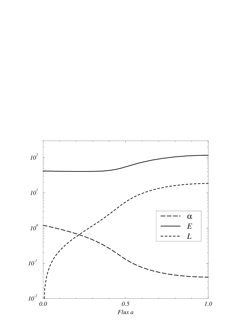
Figure 4: Example of variations of the three first integrals of the motion for a typical TTauri star (BP TAU, Bertout et al. (bertout (1988))) with respect to the magnetic flux a. they are deduced from the positions and densities of the critical points. The solid line represents the specific energy $E$, the dashed line the angular momentum $L$ and the long-dashed line the mass loss to magnetic flux ratio $\alpha$.

From Bertout et al. (bertout (1988)), we take the reference values as $\dot{M}_{\ast}=2\times 10^{-7}M_{\odot}yr^{-1}$, $M_{\ast}=0.8M_{\odot}$, $R_{\ast}=3R_{\odot}$, $T_{\ast}=9\times 10^{3}$, $n_{p}=10^{4}cm^{-3}$, and $B{\ast}=1000G$. We deduce the dimensionless input parameters ${\overline{Q}}=0.05$, ${\overline{\Omega}}=1.8$ and ${\overline{\alpha}_{0}}=0.1$. The three critical surfaces (upper panel) and corresponding densities (lower panel) are represented on Fig. 3. The lower part of the figure shows clearly the decreasing trend of the densities from the axis to the equator and stresses the differences in magnitude of the densities at the different critical points, the density at the slow point being one hundred times larger than the others. This reflects the position of the critical surfaces. On the upper part of figure 2, it can be seen that the fast and Alfvén critical surfaces definitely exhibit shapes different from spherical, particularly the fast one. One can notice that the further we go away from the axis the more the fast and the Alfvén surfaces get apart. As seen in Sakurai (saku2 (1987)) and Belcher & McGregor (belcher (1976)), as one gets closer to the equator the critical surfaces get more and more elongated along the equator. However a difference appears near the axis of rotation. In the latter cases, the critical surfaces get elongated along the pole. This is mainly due to the constancy of the angular velocity $\Omega(a)$ and of the entropy $Q(a)$. When this assumption is relaxed, equivalent behaviors have be obtained. On the other hand rotation has little effect on the slow mode critical surface which almost keeps a spherical shape. In fact the slow surface gets closer as the velocity increases, as one would expect for such a type of wave considering the increase of centrifugal acceleration near the equator. The behavior of this surface will be studied in more details in next sections. From the positions and densities of the critical points we deduce the other interesting variables of the problem, such as the first integrals of the motion $E$, $L$ and $\alpha$ as represented on Fig. 4. The specific energy seems to vary little as compared to the other quantities. Its variation is less than one percent of the mean value. Thereafter the amount of energy is slowly increasing from the value on the axis, given by Eq.(72), to an higher value on the equator. The specific angular momentum increases from the axis and then reduces its growth to level off at a value close to unity. The behavior of $\alpha$ is identical to that of the Alfvénic density as seen in Eq.(6). One should keep in mind that the value of $\alpha$ on the axis is prescribed as an input parameter.

In this subsection, we have shown a particular set of numerical solutions of the equations of this model. In the following sections we comment on the influences of the input parameters on the solutions.

4.1.3 Effects of the amplitude of the Mass Loss

Figure 5: The Alfvén surfaces for increasing $\alpha_{0}$ are shown with solid lines. Circular shapes are represented with dashed lines for comparisons with the solutions. Smaller surfaces correspond to higher values of $\alpha_{0}$ while most distorted surfaces have smaller $\alpha_{0}$. The smaller $\alpha_{0}$, the bigger the distortion and the higher the height of the Alfvèn surface on the polar axis. Small $\alpha_{0}$ can either correspond to low mass loss rate, or to high magnetic flux.

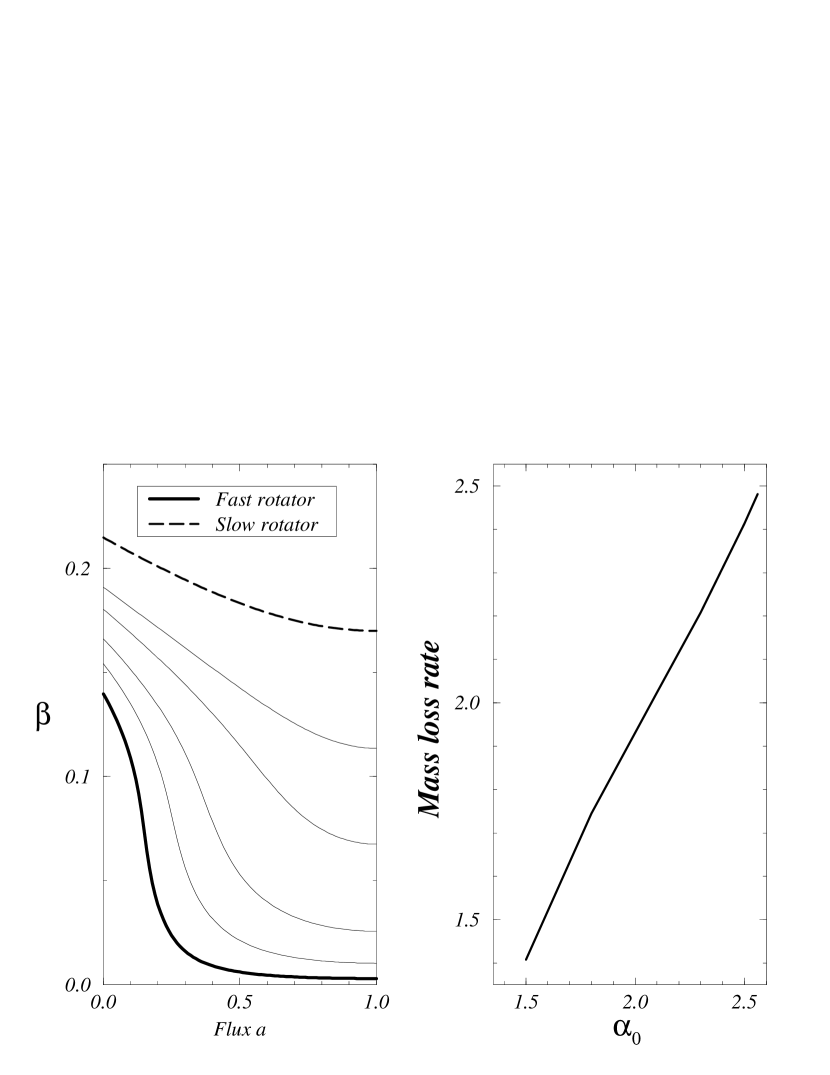
Figure 6: As shown on the left panel, $\beta$ is small compared to one for various values of $\alpha_{0}$. The upper long-dashed curve corresponds to high $\alpha_{0}$ while going down the curves, one finds solutions for smaller ratios. Those curves strengthen the assumption for our analytical calculations where $\beta$ is considered small compared to one. On the right panel, the curve indicates the total mass loss rate against $\alpha_{0}$. Notice that the slope of the curve is almost unity.

The mass loss rate $\dot{M}$ is a quantity that can be deduced from observations. In our model, it is represented by the parameter $\alpha_{0}$, the mass flux to magnetic flux ratio on the polar axis. The relation between $\alpha_{0}$ and $\dot{M}$ can be worked out a posteriori. We have calculated solutions for different $\alpha_{0}$’s, keeping for the other parameters the same value as in the previous calculations. The corresponding Alfvènic surfaces are presented in Fig. 5. Smaller surfaces correspond to high $\alpha_{0}$’s while the distorted ones correspond to smaller values. This variation is similar for all the critical surfaces. The critical surfaces strongly inflate for decreasing $\alpha_{0}$ and lose the initially spherical shape that they have at high mass loss rates. It shows that for strongly magnetized systems, the structure of the zone of acceleration gets complex.

Fig. 6 shows the evolution of $\beta$ as a function of the magnetic flux for different $\alpha_{0}$’s. Fig. 6 shows the simple relation which exists between $\alpha_{0}$ and the mass loss rate with the other input parameters fixed. In Fig. 6 the values of $\beta$, given by Eq.(13), are represented against the relative magnetic flux for a series of decreasing values of $\alpha_{0}$. When $\alpha_{0}$ is large, the behavior of $\beta$ is nearly linear but for lower values the curves start to decrease steeply and reach a low equatorial value. This strengthens one of the assumptions made to derive our analytical results, namely that the value of $\beta$ is small compared to unity. The value of $\beta$ on the axis depends directly on $Q$. If the entropy is large enough, $\beta$ can become large too and even reach unity. This would be the case for very hot outflows. The smaller $\alpha_{0}$ , the better the assumption of smallness of $\beta$ is justified. Note that the critical surfaces for magnetized rotators with small mass loss rates are strongly inflated equator-wards and are in no way similar to the quasi-spherical shape they have for rotators with large $\dot{M}$. In this section we have shown that fast and slow rotators developed different shapes of the critical surfaces. It does not seem possible to infer the solution for the fast rotator from the one obtained for a slow rotator by simple scaling scaling arguments as attempted by Shu et al. (shu94 (1994)).

4.1.4 Rotational effects

Figure 7: Effects of the angular velocity $\Omega$ on fast surfaces with parameters of a typical TTauri star. Circles are shown to visualize the distortions of the critical surfaces. These curves indicates that the faster the rotation, the bigger the distortion with respect to sphericity is. The position of the critical points on the polar axis is of course independent of the rotation.

Figure 8: The variation of the rotation parameter $\omega$ with to the magnetic flux $a$ is plotted for different values of the rotation rate $\Omega$ . The asymptotic limit of $(\frac{3}{2})^{\frac{3}{2}}$ is represented with an heavy dashed line. Lower curves represent slow rotators while upper curves stand for fast rotators. An arbitrary limit separate the two type of rotators at $\omega\sim 1$. Close to the axis, a slow rotator type behavior always remain whatever the rotation rate.

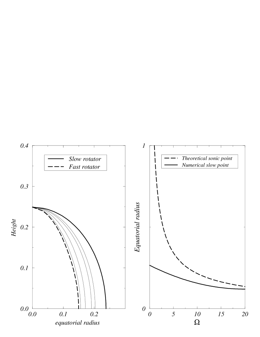
Figure 9: The shapes of the slow magneto-sonic surfaces for increasing rotation rates $\Omega$ are shown on the left panel. The slow surface has a opposite behavior compared to the fast and the Alfvèn surfaces. It deflates while $\Omega$ increases. On the right panel of the figure, the numerical solution for the magnetosonic slow point is represented with the variations of the pure sonic point with respect to the rotation rate. This shows that the slow magnetosonic point tends to the trend of the sonic point for increasing rotations.

The value of the angular velocity has a major influence on the behaviors of the solution. In Fig. 7 several Alfvénic surfaces are represented for different $\Omega$. One should notice that the central emitting object is reduced to a point and does not coincide with the first circular surface. This innermost surface corresponds to the smallest rotation rate and the other surfaces expand off the central part for larger and larger rotation rates. The faster the rotator, the larger the change in the shape of alfvénic surfaces. The effect of the rotation is strongest at the equator. The Alfvén surface remains at a finite distance from the source for finite rotation rates. The Alfvén point only goes asymptotically to infinity for ultra-fast rotators.

In Fig. 8 we present a plot of $\omega(a)$ for different rotation speeds with the same previous input parameters $Q$ and $\alpha_{0}$. The lower curves illustrates slow rotation rates and those above them correspond to increasingly larger rotation. The horizontal dashed lines represents the asymptotic limit for ultra-fast rotators where $\omega={3/2}^{3/2}\approx 1.837$. The curves pass smoothly from the region of slow to fast rotation. Once the asymptotic value for $\omega$ is nearly reached on the equator, the asymptotic region extends towards the axis for larger rotation reducing the extent of the region where the rotation parameter stays small. This region region never disappears completely, though, because obviously the polar axis itself is necessarily in the slow rotation regime.

For fast rotators the Alfvèn point is at a large distance. In this case, we see that the alfvén speed is large compared to the sound speed. At the equator the slow magneto-sonic surface as seen in Fig. 9 gets closer to the source as the rotation rate increases. The effect of the centrifugal acceleration is more and more pronounced as one reaches the equator. The slow mode speed gets closer to the sound speed, and the slow mode acquires the character of a sound wave guided along the field line. For this reason we can see the slow point on the equator moving to the source. The radius of the slow mode surface on the equator approaches the radius where the sound speed corotates with the Keplerian speed, given by:

$$r_{s}=\biggl{(}\frac{GM}{\Omega^{2}}\biggr{)}^{1/3}$$ (101)

We have represented the radius at the slow point situated on the equatorial plane as a function of increasing rotation speeds on the right panel of Fig. 9 together with the pure sonic point. It is clear that the slow magneto-sonic point tends to the sonic point. We now have a view of how all the critical surfaces behave as the rotation rate vary. Fast magneto-sonic and Alfvèn surfaces strongly inflate when rotation increases while the slow surface gets narrower to converge to a nearly cylindrical shape. It seems that an increase of $\Omega$ has almost the same effects as a decrease of $\alpha$, except that the positions of the critical points do not change on the polar axis when the rotation rate varies.

4.1.5 Thermal effects

Figure 10: Some of the thermal effects are represented on this figure. The upper panels show the variations with Q and $\gamma$ of the distance to the origin of the critical points in the equatorial plan. Below we show how $\omega$ and $\alpha$ vary. smaller entropies make the rotation parameter smaller while they produce larger ratios of mass loss rate to magnetic flux (Note that the entropy decreases from left to right). An increase of $\gamma$ have the same properties. The isothermal case produces the larger mass loss rate and as $\gamma$ increases the rotator turns to be faster.

We have assumed a polytropic equation of state. Thus the two parameters that we can vary to illustrate the thermal effects are the entropy and the polytropic index. We consider these parameters as constants as a function of flux variable $a$. In these calculations, $\Omega$ and $\alpha_{0}$ are fixed. When Q, the factor related to the entropy, decreases, the critical surfaces inflate, the rotation parameter $\omega$ increases and $\alpha$ reduces. This can be understood as follows: the more the plasma is heated, the lesser is the influence of the rotation. When the polytropic index is varied and the thermodynamics turns progressively from isothermal to adiabatic, the influence of rotation becomes more and more important. This is because the effect of gas pressure on the dynamics is maximized by an infinite thermal conduction. For most solutions the ratio of the fast mode radius to the Alfvèn radius is not very large. Thus the variations of $Q$ and $\gamma$ have a non-negligible influence but nevertheless weaker than that of varying $\Omega$ and $\alpha_{0}$. A reduction of the entropy has a similar effect to that of an increase of the polytropic index $\gamma$. The smaller the entropy, the closer the flow becomes to that of a fast rotator.

4.1.6 Limit cases

In the previous section, we have seen that the fast rotator regime is achieved before $Q$ vanishes. Similarly, all the other parameters vary in a restricted range. For example,as the rotation $\Omega$ increases, the rotation parameter $\omega$ reaches the maximum value $(\frac{3}{2})^{\frac{3}{2}}$. Numerically we find that there is an lower limit to $\alpha_{0}$ for given $\Omega$ and other parameters. To understand it, let us recall the equation $g=2GM\mu_{0}^{2}\alpha^{2}R_{A}^{3}A^{-2}$.

It has been found that

$$\omega=\frac{\Omega cos\theta\mu_{0}\alpha R_{A}^{3}}{A}.$$ (102)

So for fast rotators the Alfvènic radius tends to be almost equal to

$$R_{A}=\left(\frac{3}{2}\right)^{1/2}\left(\frac{A}{\mu_{0}cos\theta}\right)^{1/3}(\alpha\Omega)^{1/3}$$ (103)

The gravity parameter the becomes

$$g=\frac{2GM}{r_{A}vp_{A}}=\left(\frac{3}{2}\right)^{3/2}\left(\frac{2GM\mu_{0}}{Acos\theta^{2}}\right)\frac{\alpha}{\Omega}$$ (104)

Meanwhile we have found that this parameter could be expressed as

$$g=2\omega^{2}x_{s}^{3}=\frac{27}{4}x_{s}^{3}.$$ (105)

It shows that $g$ is small with respect to unity and that it does not vary much since $x_{s}$ mainly depends on the thermal parameters and not on much on the mass loss rate or the rotation rate in the case of fast rotators. It also shows that in the case of very fast rotators either the angular velocity must be very important or the mass loss rate must be small to insure that $g$ is small. One can also deduce that there is a maximum $\Omega$ for a given such as $\alpha$

$$\Omega_{max}=\omega_{max}f(\alpha_{0},Q)$$ (106)

The fitting of the numerical limits of our model where $\omega=\left(\frac{3}{2}\right)^{\frac{3}{2}}$ agrees with this result and gives

$$\Omega_{max}=\left(\frac{3}{2}\right)^{\frac{3}{2}}\left(1+\frac{Q}{2}\right)\alpha_{0}^{\frac{2}{3}}$$ (107)

Thus this shows that if the outflow is to support a given mass loss rate, it cannot rotate at any large rate. The converse is also true: if the magnetic field lines turn at a given rotation rate $\Omega$, there is a minimum mass loss rate from the central object.

4.1.7 Discussion

We have presented an extended set of solutions of the model, for constant $\Omega$ and $Q$ across the magnetic field lines. We obtain the first integrals of the motion, the components of the velocity, of the magnetic field and all the variables characterizing the flow. This study revealed some interesting properties. We have shown that an increase of $\Omega$ up to the fast rotator regime has a similar effect to a decrease of $\alpha_{0}$, or $Q$, and to an increase of $\gamma$. Fast rotators display critical surfaces which are strongly inflated equator-wards, that drastically differ from their quasi-spherical shape in the slow rotator regime. The faster the rotator, the more valid the assumption that $\beta$ is small. The influence of thermal parameters is smaller than that of rotation or mass loss rate but not negligible. Finally we have also found that a given rotation rate rate compels the mass loss rate of the outflow to have an inferior limit.

4.2 Other variations of $\Omega$ and $Q$

Figure 11: The variations of the rotation rate $\Omega$ with $a$ for the differential rotators. considered in this work. The dot-dashed line represents a Keplerian rotation. After from the bottom, one find a step-shape rotation with $\Omega$ varying from 1 to 0, a step-shape rotation from 1 to 0.5, a decreasing stellar type rotation,a constant one, a normal stellar type differential rotation and finally a step-shape rotation from 1 to 1.5.

The distribution of outflowing material in space and velocity is not well determined observationally, but some properties of such flows have still be recognized. The relatively wide spectral lines which have been measured at most places in such outflows indicate that material with a range of velocities is present on the line of sight. However, in a number of well-collimated outflows, such as NGC2024 and NGC2264G, there appears to be a shear flow, with higher velocities near the polar axis, and lower velocities at the sides of the flow (Margulis et al. (margu (1990)); Richer et al. (RHP (1992))). These observations motivated us to look for outflows with rotation rates and entropy varying with the flux variable $a$, that could reproduce such behaviors.

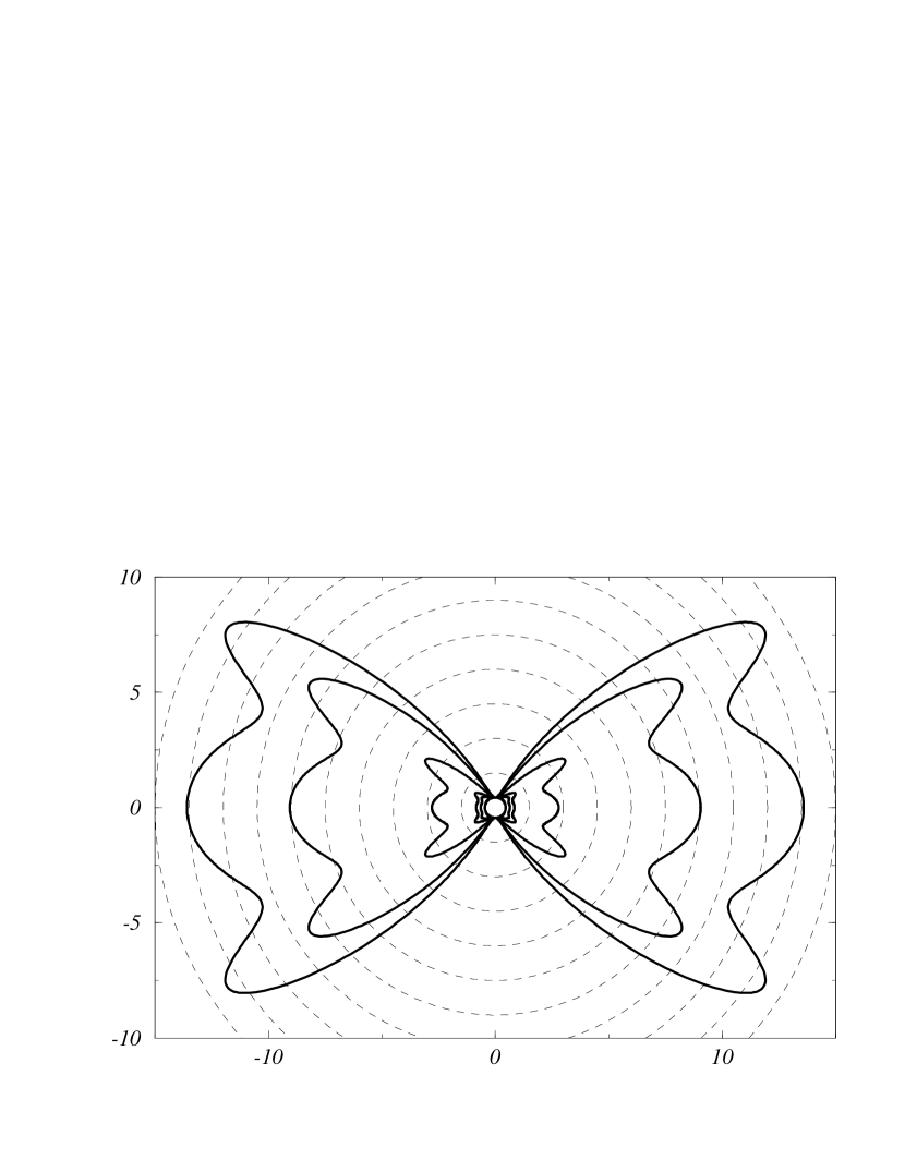
Figure 12: Fast critical surfaces for a differential rotator. In this example the rotation rate starts with a fast rotation on the axis and then reduces to a smaller rotation rate on the equator. The surfaces start just like fast rotators shown on Fig.(7) but change drastically their shapes afterwards giving this butterfly shape.

4.2.1 Non-constant $\Omega$

We now describe some specific forms of the rotation rates and discuss trends and properties that can be identified. For the rigid body rotation, the angular velocity is constant with flux $a$. The stellar-type rotation is inspired by the equation of differential rotation of the sun. We have modeled a stellar-type rotation with angular velocities larger at the equator than at the pole. We have also formulated variations of the rotation rate that could account for two components outflows such as the models of Shu et al (shu94 (1994)). A central fast flow is surrounded by a slower wind. We present two different differential rotators with this characteristics. We call them two-velocities outflows with a step-shape rotation. The analytical expressions of all these differential rotation rates can be found in appendix C. We have plotted them as functions of the magnetic flux on Fig. 11. Solutions of the problem with such profiles of rotation differ from previous ones. Critical surfaces, densities, and all the other variables, strongly vary with $a$. Fig. 12 is an illustration of of the fast critical surfaces for a two-velocities outflow. This produces “butterfly” shapes showing the possibility for two kinds of outflow with different characteristic to live side by side.

We have also plotted the solution for a central rigid rotator surrounded by a keplerian disk in Fig. 13. The central part near the axis of rotation has got a constant rotation velocity up to $a=0.3$, then $\Omega$ follows a keplerian variation. This kind of model could apply to Young Stellars Objects where the central object is launching an O-wind and the accretion disk an X-wind (see Shu et al. (shu94 (1994))).

Figure 13: Positions and densities of the the slow, Alfvénic and fast magnetosonic critical points for a fast rigid rotator surrounded by a keplerian disk.

4.2.2 Non-constant $Q$

The variation of the entropy with magnetic flux $a$ seems to have little influence on the solution in our computations, presumably because $\beta$ remained small either due to small $Q$ values or to the rapid rotator regime we imposed in several cases. Nevertheless we have studied different possibilities and only in in limit cases of the value of $Q$ and $\gamma$ the results change. In previous sections we have presented solutions for constant entropy with different values. We have also tested different variations with $a$ of the function $Q(a)$, with increasing or decreasing entropies from pole to equator and a step-shape profile. Details can be found in appendix C. The general trend is in line with the results obtained in our study of thermal effects. For either increasing or decreasing entropies, critical surfaces respectively get closer to the source or inflate outwards. For step shape variations the critical surfaces are similar to surfaces represented in Fig. 12.

5 Intermediate rotator

5.1 Analytical results

Considering $\omega$ close to unity and neglecting $\beta$ with respect to unity it is again possible to obtain analytical results for the energy and gravitation parameters. At the slow point we get

$$\epsilon=\beta y_{s}^{\gamma-1}-\frac{3}{x_{s}^{4}y_{s}^{2}}+2\omega^{2}$$ (108)

and

$$g=2\omega^{2}x_{s}^{3}.$$ (109)

At the fast point the solution for these two parameters is given by

$$\epsilon=3\omega^{4/3}$$ (110)

and

$$g=\frac{2}{x_{f}}\left(\omega^{2}+3\omega^{2/3}-\frac{4}{3}\omega^{4/3}\right).$$ (111)

It is possible to deduce equations for the positions and densities at the slow point if one considers that $y_{s}\gg y_{A}$ and $x_{s}\ll x_{A}$ and gets

$$y_{s}=\left(\frac{\beta(\gamma-1)x_{s}^{4}}{2(1+\omega^{2}x_{s}^{2})}\right)^{\frac{1}{1+\gamma}}$$ (112)

$$\frac{r_{s}}{r_{A}}=\left(\frac{\beta(\gamma-1)}{2}\right)^{\frac{1}{2(\gamma-1)}}\left(\frac{5-3\gamma}{(\gamma-1)(3\omega^{4/3}-2\omega^{2})}\right)^{\frac{\gamma+1}{4(\gamma-1)}}$$ (113)

Using the last two equations one gets a better equation for the density

$$\frac{\rho_{s}}{\rho_{A}}=\left(\frac{\beta(5-3\gamma)}{2(3\omega^{4/3}-2\omega^{2})}\right)^{\frac{1}{\gamma-1}}$$ (114)

It is also possible to get the variations of the position and density at the fast critical point. In the intermediate rotator regime, no direct simplification can be done on the positions of the critical surface, so the full set of solutions is hard to find analytically but nevertheless the solution is fully determined. Only numerical studies can help to understand the behavior of such solutions in this regime. This is what the next part intends to do with comparisons of the numerical and analytical results.

5.2 Analytical vs numerical results

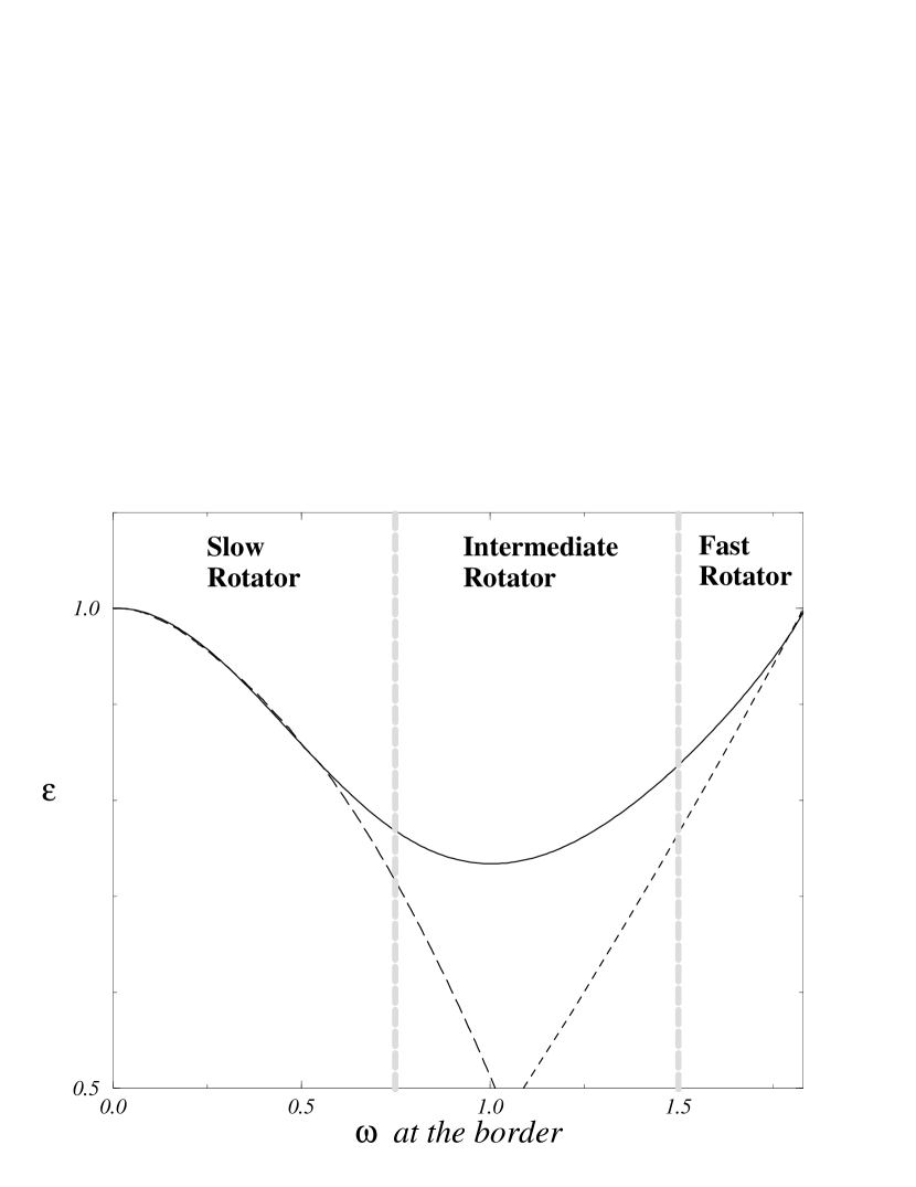
Figure 14: Comparisons of numerical results and analytical calculations of the specific energy. On the left, $\epsilon$ is represented as a function of the magnetic rotator energy $\omega$. There are good agreements for slow and very fast rotators. This is not the case of the intermediate region around $\omega=1$ that has no analytical solution. But this region is really narrow with respect to the magnetic flux a as shown on the plot on the right hand side.

The analytical solutions and the numerical results obtained for the specific energy and presented in the previous parts have been plotted in Fig.(14) for comparison. The figure shows the specific energy against the rotation parameter $\omega$. The results agree in the slow regime and in the very fast regime, as expected. The intermediate zone that we have arbitrarily situated between $\omega=0.75$ and $\omega=1.5$ shows clearly the limit of validity of the solutions for the slow and fast rotators. It shows a smooth transition between the different categories of rotators. In fact, this region is narrow in the physical space for a fast rotator since it is the transition between the central slow part of the jet close the axis of rotation and its fast part. So the analytical results are a good approximation of the numerical solution. Similar comparisons have been made for the positions and densities of the critical points with similarly positive conclusions.

6 Discussions

6.1 Comparison with other models

In a review of the theory of magnetically accelerated outflows and jets from accretion disks, Spruit (spruit (1994)) discusses how the wind structure should depend on mass flux (see also Cao & Spruit (cao (1994)) ). Using the model of Weber & Davis (wd (1967)) he concludes that when the mass flux is small, the Alfvèn radius extends far away from the origin. Our analytical and numerical results agree with these conclusions, with even more generality, since our model fills all space and does not assume any a-priori variations of the different variables. We find, using the conditions of vanishing of the differential form of the Bernoulli equation, that, if $\beta$ is small compared to unity, the Alfvèn radius on the equator can be approximated by

$$\frac{R_{A}}{R_{*}}=\frac{5}{9}\left(\frac{\alpha}{\alpha_{*}}\right)^{-1/3}.$$ (115)

For large mass loss rate, Spruit finds that the Alfvèn point does not recede arbitrarily close to the origin but reaches a minimum value. In our model when $\alpha$ becomes large the fast point can be as close as possible to the source. Following the formalism described by Spruit (spruit (1994)) and used by Sakurai (saku1 (1985)) we can deduce the relation between $\omega$ and $\alpha$ that is relevant to fast rotators, which is

$$\omega=\left(\frac{3}{2}\right)^{3/2}\left(1-\left(\frac{\alpha}{\alpha_{*}}\right)^{2/3}\right)^{3/2}$$ (116)

This solution is represented in Fig.(15) together with our numerical solutions on the equator. When $\alpha$ decreases, the two curves get closer while rotation parameter grows larger and reaches $({3}/{2})^{3/2}$ when $\alpha=0$. The ultra-fast rotator limit is clear in this case. Again we find that the larger the mass loss rate the smaller the rotation parameter. A disagreement arises with the previous formula, since it does not allow $\alpha$ to be larger than unity. This shows the limited region of validity of this analytical approximation, which nevertheless describes quite well the very fast rotator. Our analytical solutions tend to Sakurai’s results in the cold limit. In our case the slow point is defined by

$$x_{s}=\left(\frac{g}{4\omega^{2}}\right)^{1/3}.$$ (117)

This is equivalent to

$$\frac{\Omega^{2}r_{s}^{3}}{GM}=\left(\frac{v_{pA}^{2}}{2}\right)^{2}=\tilde{\omega}_{Sakurai}$$ (118)

and the specific energy is

$$\epsilon=\left(\frac{3}{2}\right)(2\omega g)^{2/3}.$$ (119)

Moreover, we can express those quantities as functions of our input variables for very fast rotators and we get

$$r_{s}^{3}=\frac{GM}{6}\left(\frac{Acos\theta^{2}}{\omega\mu_{0}\alpha}\right)^{2/3}$$ (120)

and

$$\epsilon=\left(\frac{3}{2}\right)^{5/3}\left(2GM\left(\frac{\mu_{0}\Omega\alpha}{A\cos\theta^{2}}\right)^{1/3}\right)^{2/3}.$$ (121)

Thus we find the same results as those described by Spruit in the cold limit, with more generality since we solve the transversal force balance equation on the Alfvén surface.

Figure 15: Comparisons of numerical results and analytical calculations of the relation between $\omega$ and $\alpha$ on the equator. The upper curve (solid line) represents the numerical result while the lower one (dashed line) the analytical solution as derive following the formalism of Spruit (spruit (1994)). The entropy is taken as constant. The two curves converge to each other when the rotation parameters becomes larger, which happens when $\alpha$ decreases. We find again that the bigger the mass loss rate the slower the rotation parameter.

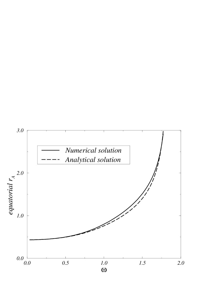
Figure 16: Comparisons of numerical results and analytical calculations of the relation between the Alfvèn radius on the equator and $\omega$. The upper curve (solid line) represents the numerical result while the lower one (dashed line) the analytical solution. The two curves are similar almost everywhere and particularly for very slow and very fast rotators.

The shapes that we have found for the critical surfaces differ from those obtained or assumed in many other models. For example, Sakurai (saku2 (1987)) found ellipsoidal shapes with his numerical studies. Blandford & Payne (bp (1982)) have chosen conical Alfvénic surfaces in their self-similar model. Chan and Henriksen (chan (1980)) and Sauty (sauty1 (1993)) used flat surfaces perpendicular to the axis of rotation. Our solutions show rather different shapes. It appears to be difficult to capture realistic behaviors by modeling the critical surfaces with simple functions.

Further developments within the framework of our model could be done to investigate the evolution of the angular momentum of solar-mass stars during pre-main and main sequence phases. Charbonneau (charbo (1992)) recently derived a braking rate from a Weber & Davis (wd (1967)) model of the solar-wind assuming a dynamo relationship where the stellar magnetic field scales linearly with the stellar angular velocity $\Omega_{\ast}$. He finds that the braking rate, $d\Omega/dt$, asymptotically scales as $\Omega_{\ast}^{3}$ at low $\Omega_{\ast}$, and as $\Omega_{\ast}^{2}$ at high $\Omega_{\ast}$. In the Weber & Davis model, the flatter $\Omega_{\ast}$-dependency of the braking rate for rapid rotators results from the change of the magnetic wind structure (Mestel (mestel (1968)), Belcher & MacGregor (belcher (1976))). That distinct braking laws apply to slow and fast rotators is further supported by observations: Skumanich’s (skuma (1972)) relationship ($\Omega_{\ast}\simeq t^{-1/2}$), which follows from an $\Omega_{\ast}^{3}$ braking law, is valid for slowly rotating dwarfs but fails for younger, more rapidly rotating zero-age main sequence star whose angular evolution is more appropriately described by an $\Omega_{\ast}^{2}$ braking law (Mermilliod & Mayor (mermi (1990))). Thus our work takes place in a context of interesting studies and some further investigations should be done in this direction.

6.2 A criterion for the classification of rotators

With respect to the previous results, it has been interesting to neglect the effects of the thermal parameters and only to look at those of the rotation, of the magnetic field and of the mass loss rate. It has been shown that an increase of $\Omega$ has effects similar to those of a decrease of $\alpha_{0}$, all the other parameters being fixed. This suggests that the ratio $\frac{\Omega}{\alpha_{0}}$ might be relevant for a study of magnetized rotators. That is the reason why we have plotted the relation between the ratio ${\Omega}/{\alpha_{0}}$ and $\omega$. First this gives a global relation between the input parameters of the model that can be related to physical parameters given by observations (See appendix C) and the variable $\omega$ that is a result of the calculation.

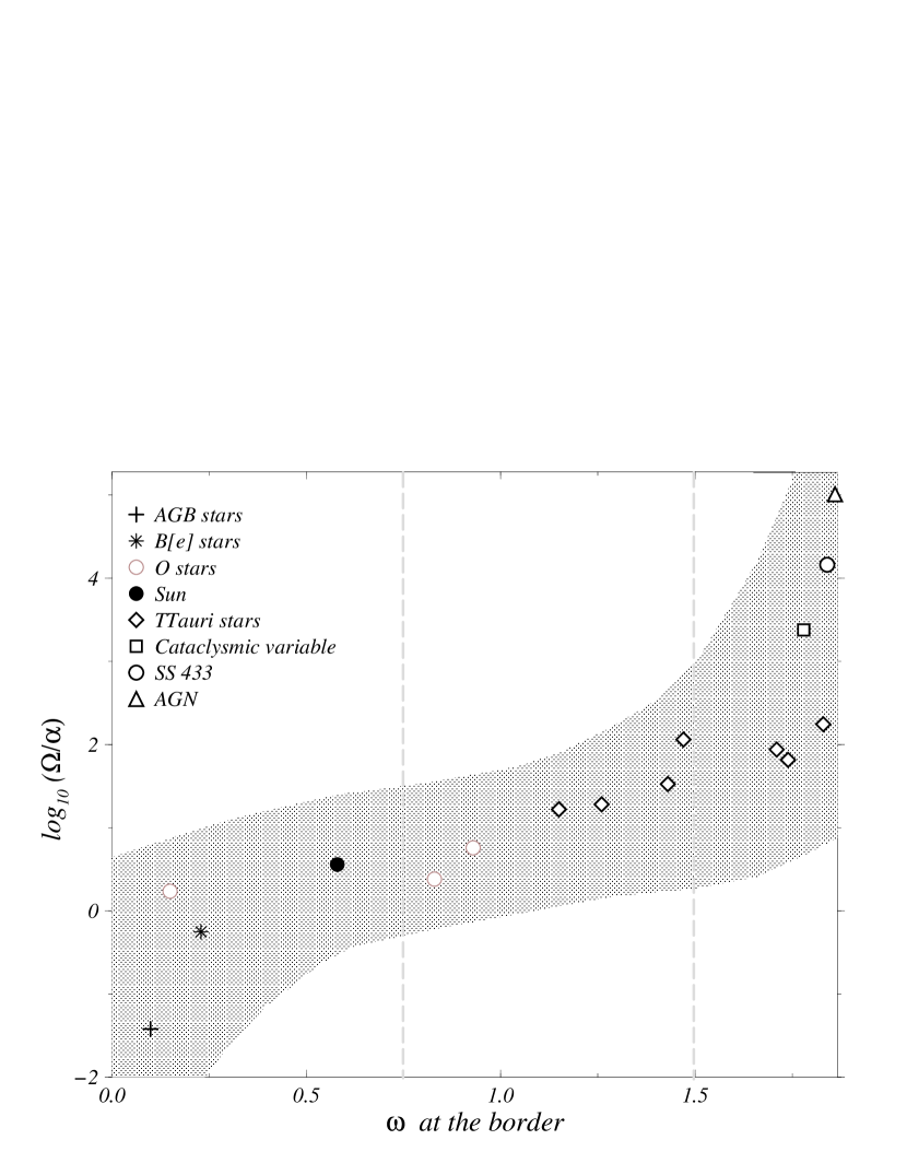
Figure 17: Classification of the magnetic rotators. the logarithm of the ratio $\frac{\Omega}{\alpha_{0}}$ given by the observational literature is plotted against the rotation parameter $\omega$ obtained by the calculation for several astrophysical objects. The grey zone represents the region of uncertainty over the input parameters. The two vertical thin dashed line shows the approximate limits between slow, intermediate and fast rotators. The limit for ultra-fast rotators is at $\omega=(\frac{3}{2})^{3/2}\approx 1.837$.

We find a continuity between slow and fast rotators. Slow rotators correspond to $\omega\ll 1$. Since this class contains the Solar wind, winds of of B[e] stars, AGB stars, it can be identified with winds in general. In the intermediate regime that arbitrarily corresponds to $0.75<\omega<1.5$ we find both O stars and TTauri stars. This region clearly shows a smooth transition between slow and fast rotators. In the fast rotator zone where $\omega$ is close to $\left(\frac{3}{2}\right)^{3/2}$ only object with jets, i.e. outflows of TTauri stars, of cataclysmic variable, of microquasars such as SS433 and of active galactic nuclei, are to be found. This shows two main types of objects, winds and jets with a transition in between. One should notice an important difference between the TTauri stars belonging to the intermediate zone and those in the fast rotator regime. They have larger mass loss rate ($>10^{-7}M_{\odot}yr^{-1}$) compared to the other ones (¡$10^{-7}M_{\odot}yr^{-1}$). This could be due to a difference of ages for these TTauri stars. This suggests that $\dot{M}$ and $\omega$ are closely related. Then our model could provide a tool to see the evolution of this type of object and to classify them.

From the input parameters related to astrophysical quantities given by observations and with the results of the model, we can classify outflows of magnetized rotators into slow, intermediate and fast rotators. We have also computed solutions for planetary nebulae and Wolf-Rayet stars but, since the origin of their wind is mainly radiative, they should not be compared with the other objects. Nevertheless the numerical results obtained for these types of astronomical objects shows that they are definitely slow rotators following our classification.

6.3 Limits of the model

Our model possesses several advantages. First it is not self-similar and secondly it can accept any boundary conditions. Moreover the simplifications allows us to find fully analytical solutions in limit cases and systems of equations which are easy to solve numerically in all cases. The model is not simply a continuous set of closely packed Weber-Davies solutions but it is made coherent with the Alfvén regularity condition on the Alfvén surface, which retains part of the cross-field balance. It also gives the possibility to solve the Bernoulli equation from the source to the fast point and finally the asymptotic resolution of the outflow is possible (See Lery et al. (1998b )) giving the possibility to relate the properties of the source to the asymptotic behavior of the outflow.

The main weaknesses however are the following. First our model does not give an exact solution to the system of coupled Bernoulli and transfield equations. Secondly the geometry of the magnetic field lines is idealized. This latter difficulty could be avoided by iterating on the field geometry.

7 Conclusions

In this Paper, we have proposed a simplified set of the equations for rotating magnetized outflows by assuming the shape of the poloidal magnetic field lines up to the fast magneto-sonic point. Rather than solving the equilibrium perpendicular to the flux surfaces everywhere, solutions are found at the Alfvèn point where it takes the form of the Alfvèn regularity condition and at the base of the flow. This constrains the transfield equilibrium in that the Alfvèn regularity condition is imposed and the regularity of the magnetic surfaces at the Alfvèn critical surface is ensured. In our model, the outflow is parameterized by $\Omega(a)$, $Q(a)$ and $\alpha_{0}$ which is related to the mass loss rate. We deduce three first integrals of the motion, the specific angular momentum, the specific energy and the mass flux to magnetic flux ratio on a magnetic surface from criticality and Alfvèn regularity conditions. Different profiles for the variation of the entropy and the rotation rate with respect to the magnetic flux have been considered. The simplifications of the model allow to find analytical behaviors of the first integrals as well as the shape of the critical surfaces in limiting cases. We found good agreement between analytical and numerical solutions. For a given entropy, magnetic rotators can be characterized by the ratio of the rotation rate and the magnetic to mass flux ratio on the polar axis, i.e. $\Omega/\alpha_{0}$. This latter ratio is given by the boundary conditions.

Given the properties of the central emitting object, the model allows us to compute its corresponding dimensionless rotation parameter $\omega$. Rotators can be defined as slow, intermediate or fast according to whether $\omega$ is much less or close to unity or near its maximum value for fast rotators, $(\frac{3}{2})^{\frac{3}{2}}$.

Slow rotators have quasi-spherical critical surfaces and a fast surface close to the Alfvén surface, their properties strongly depend on the heating.

Fast rotators have distorted critical surfaces and a fast surface far from the Alfvén surface (approaching infinity only in the zero temperature limit). Their properties strongly depend on the magnetic flux and the rotation rate yet always retain a slow rotator behavior near the axis of rotation. They display a slow mode that acquires the character of a sound wave as the rotation rate increases and are limited, in the present conical model, by $\omega=\frac{3}{2}^{\frac{3}{2}}$.

For all types of rotators, it is found using conical shapes that the mass loss rate has a lower limit for a given rotation rate. The strongest effects on solutions are due to the rotation with respect the thermal and mass loss rate effects for typical astrophysical values. Given the angular velocity $\Omega(a)$ and the specific entropy $Q(a)$, the solutions for the last first integrals of the motion, namely the specific energy $E$, the specific angular momentum $L$ and the mass to magnetic flux ratio $\alpha$ can be determined numerically and in some limiting cases analytically. Non-constant rotation cases allow two-velocities outflow types, with possibly more complex solutions for different profiles of angular velocity and entropy.

This simplified model makes it possible to investigate the structure of outflows far from the magnetized rotator source, unconstrained by type of boundary conditions, and without the need for self-similar assumptions. How outflows extend into the asymptotic region constitutes the subject of the study of Paper II (Lery et al.(1998b ). Paper III (Lery et al.(1998c ) will deal with a linear stability analysis of the asymptotic equilibria.

Appendix A Cold rotators

In the conical case it useful to have the simplified equations for $\beta\ll 1$ since numerically we have seen that this assumption is quite acceptable as long as Q(a) is not to big. These equations allow easy analytical works. Particularly for fast and slow rotators, one just have to study the limit of variation of $\omega$ to get the equations for positions and densities for the critical points. Thus we have

$$y_{s}=\left({\frac{\beta\left(\gamma-1\right)x_{s}^{4}}{2\left(1+\omega^{2}x_{s}^{2}\left(1-x_{s}^{2}\right)^{2}\right)}}\right)^{\frac{-1}{\gamma+1}}$$ (122)

$$y_{f}={\frac{1}{1+\left(\omega x_{f}\left(x_{f}^{2}-1\right)\right)^{\frac{2}{3}}}}$$ (123)

One can deduce a reduced form for the relative energy and the relative gravity that only depend on $x_{s}$, $x_{f}$ and on two parameters $\omega,\beta$

$$\epsilon = \beta\left(1+\omega^{\frac{2}{3}}x_{f}^{2}(1-x_{f}^{-2})^{\frac{2}{3}}\right)^{1-\gamma}$$ (124)

$$+\frac{6\omega^{\frac{4}{3}}}{\left(1-x_{f}^{-2}\right)^{\frac{2}{3}}}-3\omega^{\frac{4}{3}}\left(1-x_{f}^{-2}\right)^{\frac{4}{3}}$$

$$+x_{f}^{-2}\{-\omega^{2}-6\omega^{\frac{2}{3}}\left(1-x_{f}^{-2}\right)^{\frac{2}{3}}$$

$$+\frac{3\omega^{\frac{2}{3}}}{\left(1-x_{f}^{-2}\right)^{\frac{4}{3}}}-\frac{4\omega^{\frac{4}{3}}}{\left(1-x_{f}^{-2}\right)^{\frac{2}{3}}}\}$$

$$+x_{f}^{-4}\{-3-\frac{2\omega^{\frac{2}{3}}}{\left(1-x_{f}^{-2}\right)^{\frac{4}{3}}}-\frac{2\omega^{\frac{4}{3}}}{\left(1-x_{f}^{-2}\right)^{\frac{2}{3}}}\}$$

$$+x_{f}^{-6}\{\frac{-\omega^{\frac{2}{3}}}{\left(1-x_{f}^{-2}\right)^{\frac{4}{3}}}\}$$

$$\epsilon = \omega^{2}(2-3x_{s}^{2})$$ (125)

$$+\left(\frac{\beta\left(\gamma-1\right)x_{s}^{4}}{2\left(1+\omega^{2}x_{s}^{2}(1-x_{s}^{2})^{2}\right)}\right)^{\frac{2}{\gamma+1}}$$

$$\left(\frac{5-3\gamma}{(\gamma-1)x_{s}^{4}}\right)$$

$$+\left(\frac{\beta\left(\gamma-1\right)x_{s}^{4}}{2\left(1+\omega^{2}x_{s}^{2}(1-x_{s}^{2})^{2}\right)}\right)^{\frac{2}{\gamma+1}}$$

$$\left(\frac{\omega^{2}x_{s}^{2}(1-x_{s}^{2})\{2(1-x_{s}^{2})-(\gamma-1)(3x_{s}^{2}+1)\}}{(\gamma-1)x_{s}^{4}}\right)$$

$${\frac{g}{2}} = \frac{2\omega^{\frac{4}{3}}}{({\frac{r_{A}}{r_{f}}})}\left(1-\frac{1}{\left(1-({\frac{r_{A}}{r_{f}}})^{2}\right)^{\frac{2}{3}}}\right)$$ (126)

$$+({\frac{r_{A}}{r_{f}}})\left(\omega^{2}-\frac{\omega^{\frac{2}{3}}}{\left(1-({\frac{r_{A}}{r_{f}}})^{2}\right)^{\frac{4}{3}}}+\frac{4\omega^{\frac{2}{3}}}{\left(1-({\frac{r_{A}}{r_{f}}})^{2}\right)^{\frac{2}{3}}}\right)$$

$$+({\frac{r_{A}}{r_{f}}})^{3}\left(\frac{2}{\left(1-({\frac{r_{A}}{r_{f}}})^{2}\right)^{\frac{4}{3}}}+\frac{2\omega^{\frac{4}{3}}}{\left(1-({\frac{r_{A}}{r_{f}}})^{2}\right)^{\frac{2}{3}}}\right)$$

$$+({\frac{r_{A}}{r_{f}}})^{5}\left(\frac{\omega^{\frac{2}{3}}}{\left(1-({\frac{r_{A}}{r_{f}}})^{2}\right)^{\frac{4}{3}}}\right)$$

$$\frac{g}{2} = \omega^{2}x_{s}^{3}+\left(\frac{\beta\left(\gamma-1\right)x_{s}^{4}}{2\left(1+\omega^{2}x_{s}^{2}(1-x_{s}^{2})^{2}\right)}\right)^{(\frac{2}{\gamma+1})}$$ (127)

$$\left(\frac{2+\omega^{2}x_{s}^{2}(1-x_{s}^{2})(1+x_{s}^{2})}{x_{s}^{3}}\right)$$

Appendix B Profiles of $\Omega(a)$ and $Q(a)$

Definitions of parameters:

• $\Omega_{0}$: angular velocity

• $a$: magnetic flux

• $N$: large integer

• $B$ and $C$: constants

• $C_{1}$ and $C_{2}$: constants with $C_{1}+C_{2}\leq 1$

Differential rotators

• Rigid body rotation

  $$\Omega=\Omega_{0}$$ (128)

• Keplerian rotation

  $$\Omega = \Omega_{0}(\frac{({1-a}{\sqrt{a(2-a)}})^{3/2}}{1+\exp(-Na+N/10)}$$ (129)

  $$+\frac{1}{(1+\exp(-Na+N/10))})$$

• Stellar type rotation

  $$\Omega=\Omega_{0}(1-B\sin^{2}\theta-C\sin^{4}\theta)$$ (130)

  with

  $$\theta=\arccos\left(\sqrt{a(2-a)}\right)$$ (131)

• Decreasing stellar type rotation

  $$\Omega=\Omega_{0}(1-B\cos^{2}\theta-C\cos^{4}\theta)$$ (132)

• Two velocities rotation ($\Omega_{0}$-0)

  $$\Omega=\frac{\Omega_{0}}{\exp(N(a-\frac{1}{2}))+1-\exp(-\frac{N}{2})}$$ (133)

• Two velocities rotation ($\Omega_{0}$-$\Omega_{1}$)

  $$\Omega=\Omega_{0}\left(C_{1}+\frac{C_{2}}{\exp(N(a-\frac{1}{2}))+1-\exp(-\frac{N}{2})}\right)$$ (134)

Variations of $Q(a)$

• Constant entropy

  $$Q=Q_{0}$$ (135)

• Two entropies $(Q_{0}-\frac{Q_{0}}{2})$

  $$Q=Q_{0}\left(0.5+\frac{0.5}{\exp(N(a-\frac{1}{2}))+1-\exp(-\frac{N}{2})}\right)$$ (136)

• Increasing entropy

  $$Q=Q_{0}(1-B\sin^{2}\theta-C\sin^{4}\theta)$$ (137)

  with

  $$\theta=\arccos\left(\sqrt{(2-a)}\right)$$ (138)

• Decreasing entropy

  $$\Omega=\Omega_{0}(1-B\cos^{2}\theta-C\cos^{4}\theta)$$ (139)

Appendix C Examples of input parameters for astrophysical objects

Table 1: Examples of input parameters for astrophysical objects

Object type	$log{(\frac{\Omega}{\alpha})}$	$\omega$	${\overline{\Omega}}$	${\overline{\alpha}}$	${\overline{Q}}$	$\dot{M}$	$M$	$R$	$T$	$n$	$B$
						$(M_{\odot}yr^{-1})$	$(M_{\odot})$	$(R_{\odot})$	(K)	$(cm^{-3})$	(G)
AGB a	-1.70	0.07	0.001	0.05	0.26	$2\times 10^{-6}$	5	500	2800	$10^{10}$	0.1
B[e] b	-0.53	0.20	0.5	1.7	0.2	$2\times 10^{-6}$	37	86	$2\times 10^{4}$	$10^{10}$	1
O5 V c	-0.05	0.12	7.0	7.85	20.4	$2\times 10^{-10}$	1	1	$2\times 10^{6}$	$10^{8}$	1
O3 IIIc	0.10	0.80	0.56	0.44	0.8	$6.2\times 10^{-6}$	50	19.7	$6.5\times 10^{4}$	$10^{10}$	$2\times 10^{2}$
O3 IIIc	0.48	0.91	0.56	0.18	0.8	$6.2\times 10^{-6}$	50	19.7	$6.5\times 10^{4}$	$10^{10}$	$1.6\times 10^{3}$
Sun d	0.26	0.55	3.1	1.7	2.1	$10^{-14}$	1	1	$10^{6}$	$10^{10}$	$10^{3}$
DF Taue,h	0.94	1.12	0.8	0.09	0.07	$1.3\times 10^{-7}$	2	2.5	$4\times 10^{3}$	$10^{4}$	$2\times 10^{3}$
GG Taue	1.00	1.23	1.0	0.1	0.03	$4\times 10^{-7}$	0.8	3.5	$10^{4}$	$10^{8}$	$2\times 10^{3}$
BP Taue	1.24	1.41	1.8	0.1	0.05	$2\times 10^{-7}$	0.8	3.0	$9\times 10^{3}$	$10^{4}$	$1\times 10^{3}$
RY Taue	1.53	1.71	2.2	0.065	0.02	$7.5\times 10^{-8}$	2	2.7	$8\times 10^{3}$	$10^{4}$	$1\times 10^{3}$
DS Taue	1.66	1.68	2.9	0.022	0.05	$6.5\times 10^{-8}$	1	1.8	$9\times 10^{3}$	$10^{6}$	$2\times 10^{3}$
T Tau e	1.78	1.44	1.23	0.02	0.07	$1.1\times 10^{-7}$	2	4	$7\times 10^{3}$	$10^{10}$	$2\times 10^{3}$
SU Aure	1.96	1.80	50	0.05	3.0	$2\times 10^{-8}$	2.25	3.6	$2\times 10^{5}$	$10^{8}$	300
C.V. f	3.10	1.75	11	0.008	1.4	$2\times 10^{-10}$	1	1.2	$10^{6}$	$7\times 10^{13}$	$10^{6}$
SS 433g	3.88	1.81	65	0.009	0.1	$10^{-4}$	10	0.2	$10^{5}$	$10^{10}$	$10^{9}$
A.G.N.g	4.73	1.83	160	0.003	0.7	$10^{-4}$	$10^{9}$	150	$2\times 10^{5}$	$2\times 10^{6}$	$10^{4}$
a Livio (livio (1994)).
b Cassinelli et al. (cassi (1989)).
c Mc Gregor (mcgregor (1996)).
d Priest (priest (1987)).
e Bertout et al. (bertout (1988)).
f Murray & Chiang (murray (1996)).
g Bremer (bremer (1996)).
h Thiébaut et al. (thieb (1995)).

References

- (1) Belcher, J.W., MacGregor, K.B., 1976, ApJ 210, 498.
- (2) Bertout, C., et al., 1988, ApJ, 330, 350.
- (3) Blandford, R.D., Payne, D.G., 1982, MNRAS, 199, 883.
- (4) Bremer, M., 1996, cghr.conf. B., Astrophysics and space science library, ed. Bremer, M. (Dordrecht: Kluwer).
- (5) Cao, X., Spruit, H.C., 1994, A&A, 287, 80.
- (6) Cassinelli, J.P., et al., 1989, in Physics of luminous blue variables, ed. K. Davidson et al. (Dordrecht:Kluwer), 121.
- (7) Chan, K.L., Henriksen, R.N., 1980, ApJ, 241, 534.
- (8) Charbonneau, P., 1992, in Seventh Cambridge Workshop on Cool stars, Stellar systems and the Sun, ASP Conf. Ser., ed. M.S. Giampapa & J.A. Bookbinder, 26, 417.
- (9) Contopoulos, J., Lovelace, R.V.E., 1994, ApJ, 429, 139.
- (10) Ferreira, J., Pelletier, G., 1993a, A&A, 276, 625.
- (11) Ferreira, J., Pelletier, G., 1993b, A&A, 276, 637.
- (12) Ferreira, J., 1997, A&A, 319, 340.
- (13) Fiege, J.D., Henriksen, R.N., 1996, MNRAS, 281, 1038.
- (14) Hartmann, L., Mc Gregor, K.B., 1982, ApJ, 259, 180.
- (15) Henriksen, R.N., Valls-Gabaud, D., 1994, MNRAS, 266, 681.
- (16) Heyvaerts, J., Norman, C., 1989, ApJ, 347, 1055.
- (17) Kennel, C.F., Fujimura, F.S., Okamoto, I., Geophys. Astrophys. Fluid Dynamics, 1983, 26, 147.
- (18) Königl, A., 1989, ApJ , 342, 208.
- (19) Koupelis, T., Van Horn, H.M., 1989, ApJ , 342, 146.
- (20) Koupelis, T., 1990, ApJ , 363, 79.
- (21) Lery, T., Heyvaerts, J., Appl, S., Norman, C.A., 1998b, A&A, in preparation (Paper II).
- (22) Lery, T., Appl, S., Heyvaerts, J., 1998c, A&A, in preparation (Paper III).
- (23) Li, Z. Y., 1995, ApJ, 444, 848.
- (24) Livio, M., 1994 in Circumstellar Media in late stages of stellar evolution, ed. R. Clegg et al. (Cambridge Univ. Press), 35.
- (25) Mc Gregor, K.B., 1996, in K.C. Tsinganos (ed.), Solar & Astrophysical Magnetohydrodynamic Flows, Kluwer, 301.
- (26) Margulis, M., et al., 1990, ApJ, 352, 615.
- (27) Mermilliod, J.C., Mayor, M., 1990, A&A, 237, 61.
- (28) Mestel, L., 1968, MNRAS, 138, 359.
- (29) Mestel, L., Spruit, H.C., 1987, MNRAS, 226, 57.
- (30) Michel, F.C., 1969, ApJ, 158,727.
- (31) Murray, N., Chiang, J., 1996, in Nature, 382, 789.
- (32) Najita, J. R., Shu, F.H., 1994, ApJ, 429, 808.
- (33) Okamoto, I., 1978, MNRAS, 185, 69.
- (34) Ouyed, R., 1995, BAAS, 27, 1317.
- (35) Ouyed, R., Pudritz, R.,1997, ApJ, 482, 712.
- (36) Parker, E.N., 1963, Interplanetary dynamical processes, New York, Interscience Publishers.
- (37) Pelletier, G., Pudritz, R.E., 1992, ApJ, 394, 117.
- (38) Priest, E.R., 1987, Solar magneto-hydrodynamics, D. Reidel publishing Company (Dordrecht).
- (39) Pudritz, R. E., Norman, C. A., 1986, ApJ, 301, 571.
- (40) Richer, J.S., Hills, R.E., Padman, R., 1992, MNRAS, 254, 525.
- (41) Rosso, F., Pelletier, G., 1994, A&A, 287, 325.
- (42) Sakurai, T., 1985, A&A, 152, 121.
- (43) Sakurai, T., 1987, PASJ, 39, 821.
- (44) Sauty, C. 1993 PhD Thesis, University of Paris VII.
- (45) Sauty, C., Tsinganos, K., 1994, A&A, 287, 893.
- (46) Shu, F.H., Lizano, S. Ruden, S.P. and Najita, J. 1988, ApJ, 328, L19
- (47) Shu, F.H., Najita, J., Ostriker, E., Wilkin, F., Ruden, S. and Lizano, S., 1994, ApJ, 429, 781.
- (48) Skumanich, A., 1972, ApJ, 171, 565.
- (49) Spruit, H.C., 1994, Cosmical Magnetism, NATO ASI Series C. eds. D. Lynden-Bell (Kluwer), 422, 33.
- (50) Suess, S.T., Nerney, S.F., 1973, ApJ, 184, L17.
- (51) Thiébaut, E., Balega, Y., Balega, I., Belkine, I., Bouvier, J., Foy, R., Blazit, A. and Bonneau, D., 1995, A&A, 304, 17.
- (52) Tsinganos, K., Sauty, C., 1992, A&A, 255, 405.
- (53) Tsinganos, K., Trussoni, E., 1991, A&A, 249, 156.
- (54) Uchida, Y., Shibata, K., 1985, PASJ, 37, 515.
- (55) Wardle, M., Königl, A., 1993, ApJ, 410, 218.
- (56) Weber, E.J., Davis, L., 1967, ApJ, 148, 217.