Outflows from magnetic rotators

Abstract

The asymptotic structure of outflows from rotating magnetized objects confined by a uniform external pressure is calculated. The flow is assumed to be perfect MHD, polytropic, axisymmetric and stationary. The well known associated first integrals together with the confining external pressure, which is taken to be independent of the distance to the source, determine the asymptotic structure. The integrals are provided by solving the flow physics for the base within the framework of the model developed in Paper I (Lery et al. 1998), which assumes conical geometry below the fast mode surface, and ensures the Alfvén regularity condition. Far from the source, the outflow collimate cylindrically. Slow (i.e. with small rotation parameter $\omega$) rigid rotators give rise to diffuse electric current distribution in the asymptotic region. They are dominated by gas pressure. Fast rigid rotators have a core-envelope structure in which a current carrying core is surrounded by an essentially current free region where the azimuthal magnetic field dominates. The total asymptotic poloidal current carried away decreases steadily with the external pressure. A sizeable finite current remains present for fast rotators even at exceedingly small, but still finite, pressure.

1 Introduction

Jets from young stellar objects (YSO) and active galactic nuclei (AGN) are most likely launched magnetically. Various approaches have been used to describe the stationary configuration of magnetically collimating winds governed by the Grad-Shafranov equation (e.g. Lery et al. lery1 (1998) hereafter Paper I, and references therein). Magnetized rotating MHD winds can be accelerated from an accretion disk (“Disk wind”, Blandford & Payne bp (1982), Pelletier & Pudritz pellpud (1992)), at the disk-magnetosphere boundary (“X-winds”, Shu et al. shul (1988), shu94 (1994), shu97 (1997)) or directly from the star itself by combined pressure and magneto-centrifugal forces (“Stellar wind”, Weber & Davis wd (1967), MacGregor macg (1996) and reference therein). In order to make the system of equation more tractable angular self-similarity has been often employed for non rotating magnetospheres (Tsinganos & Sauty tsin1 (1992)), and outflows from spherical rotating objects (Sauty & Tsinganos sautytsing (1994), Trussoni et al. (trussoni (1997)), Tsinganos et Trussoni tsin2 (1991)). Cylindrical self-similarity has also been used for magnetized jets (Chan & Henriksen chanh (1982)), and spherical self-similarity for disk winds (Blandford & Payne bp (1982), Henriksen & Valls-Gabaud henrik (1994), Fiege & Henriksen fiege (1996), Contopoulos & Lovelace conto (1994), Ferreira & Pelletier ferr1 (1993), Ferreira ferr3 (1997), Ostriker ostriker (1997), Lery et al. lhf (1999)). However this assumption presents boundary condition restrictions. Several numerical simulations, such as Ouyed & Pudritz ouyedp (1997), have been made in order to understand the formation of magnetized jets from keplerian discs, but due to computational limitations only a few cases have been studied. One should also note that pure hydrodynamic collimation could be effective at producing jets (Frank & Mellema FM (1996)). High velocity outflows from YSO and AGN are observed to be highly collimated. Heyvaerts & Norman (HN (1989)) have discussed how streamlines asymptotically develop in winds with different properties without considering confinement by any external medium (see also Heyvaerts HN2 (1996)). They have shown that winds which carry a non-vanishing Poynting flux and poloidal current to infinity must contain a cylindrically collimated core, whereas other winds focus parabolically. Li et al. (liCB (1992)) showed how the formation of weakly collimated, conical flows depends on the shape of the poloidal field near the Alfvén surface. The transition from weakly collimated flows to highly collimated jets has been also studied by Sauty & Tsinganos (sautytsing (1994)).

Close to the Source

In Paper I, a model for the stationary structure of the inner part of the flow has been proposed based on the assumption that the magnetic surfaces possess a shape which is a priori known inside the fast critical surface. As a first approximation magnetic surfaces were taken to be cones. Unlike the Weber-Davis type models, the balance of forces perpendicular to the magnetic surfaces is taken into account on the Alfvénic surface through the Alfvén regularity condition. This, together with the criticality conditions determine the three unknown constants of the motion, that are conserved along magnetic surfaces $a$, namely the specific energy $E(a)$, the specific angular momentum $L(a)$ and the mass to magnetic flux ratio $\alpha(a)$. Once these first integrals are determined, the asymptotic cylindrically collimated flow is uniquely determined. The solutions are parameterized by the angular velocity of the magnetic field lines $\Omega(a)$, the specific entropy at the base $Q(a)$ and by the mass flux to magnetic flux ratio on the polar axis $\alpha_{0}$. According to the rotation parameter $\omega=\frac{\Omega r_{A}}{v_{PA}}$ the objects can be classified as slow ($\omega<<1$), fast ($(\frac{3}{2})^{3/2}-\omega<<1$) or intermediate (other values of $\omega$ ranging between 0 and $(\frac{3}{2})^{3/2}$) rotators. Critical surfaces are nearly spherical for slow rotators, but become strongly distorted for rapid rotators, giving rise to important gradients of density and velocity that should consequently effect asymptotic quantities. This simplified model makes it possible to investigate the structure of outflows far from the magnetized rotator source without the need for self-similar assumptions. The price to pay for that is that the model does not give an exact, but only an approximate, solution because the transfield equation is not solved everywhere, but only at a few special places.

How outflows behave in the asymptotic region constitutes the subject of the study of this paper which also focuses on the study of the asymptotic electric current and addresses the question of the asymptotic collimation of the different classes of rotators found in Paper I. In this paper, we present a model where the collimated jet is assumed to be in pressure equilibrium with an external medium whose properties are independent of the distance to the source. The question of the asymptotic electric current is a major concern for jets that will be investigated.

We structure our paper as follows: In §2, we present the equations governing the asymptotic equilibrium, and their boundary conditions. Solutions and parameter studies are presented in §3. We derive analytical and numerical solutions for the asymptotic electric current in §4. Finally, in§5, we discuss the implications of our analysis and we summarize our results in §6.

2 The Analytical Model

2.1 The Jet Base

Figure 1: Schematic representation of the magnetic structure of the model. The magnetic surfaces projected in the poloidal plane are conical within the fast magnetosonic surface and connect to the cylindrical asymptotic region. In this part, the outflow is surrounded by an external confining medium. S, A and F denote the slow magnetosonic, the Alfvén and the fast magnetosonic surfaces, respectively.

Magnetic surfaces in the inner region are assumed to be conical up to the fast magnetosonic surface. The flow eventually becomes cylindrical due to confinement by uniform external pressure (Fig. 1). Henceforth we work in the cylindrical coordinate system ($r$,$\phi$,$z$) whose axis coincides with the symmetry-axis. Each flux surface is labeled by the flux function $a(r,z)$ proportional to the magnetic flux through a circle centered on the axis passing at point $r$, $z$. The physical flux is $2\pi a$. The equatorial value of this function is A. In addition to being steady and axially symmetric, we further constrain the mass density $\rho$ of the flow to be related to the gas pressure $P$ by a polytropic equation of state $P=Q(a)\rho^{\gamma}$. We refer to $Q(a)$ as the ”specific entropy” of the flow (though it would be related to it only for adiabatic flows). The constant $\gamma$ is the polytropic index which is considered to be constant. The specific entropy $Q(a)$, the angular velocity of the magnetic field lines $\Omega(a)$ and the mass to magnetic flux ratio $\alpha(a)$ are constant along any flux surface $a$, and entirely determine the outflow in the conical region. The total energy $E(a)$, the total angular momentum $L(a)$, and the ratio of matter to magnetic flux $\alpha(a)$, expressed through the density at the Alfvén point $\rho_{A}(a)$, are also conserved along the flux surfaces and follow from the regularity of the solution at the Alfvénic and fast and slow magnetosonic surface.

2.2 The Intermediate Zone

The MHD flow in regions causally disconnected from the base region has no back-reaction on its properties in this region. It is known that this causally disconnected region starts at the so-called fast limiting characteristic (Tsinganos et al. tsin3 (1996)), which is usually situated downflow from the fast magnetosonic surface. The flow in the causally disconnected region has no influence on the values assumed by the three first integrals which are not a-priori known. The flow between the fast mode critical surface and the fast mode limiting separatrix would have some influence on their determination if the shape of magnetic surfaces between the source object and the fast limiting separatrix were self-consistently calculated by solving exactly the transfield equation. However, in the present simplified and fixed base geometry, these first integrals are entirely determined from sub-fast surface regions and there is no need, for their determination, nor for that of the asymptotic structure, to calculate the geometry of magnetic surfaces in the intermediate region between the fast critical surface and the fast mode limiting separatrix. The latter is anyway presumably located not much further away from it and we do not expect large geometrical changes as compared to the base region. The lack of complete self-consistency of our model is therefore mainly contained in our assumption of base conical geometry. The fact that the shape of surfaces is not calculated downflow from the fast surface in regions were field curvature is still present, i.e. where poloidal field lines are dashed in Fig. 1, does not add any supplementary inaccuracy.

The shape of the magnetic surfaces shown in Fig. 1 are similar, to some extent, to shapes obtained by some previous studies already performed for a self-consistent calculation of the shape of the poloidal field lines. Trussoni et al. (trussoni (1997)) have prescribed similar types of the magnetic surfaces and then integrated the MHD equations from the base all the way to infinity. Such case corresponds to meridionally self-similar MHD outflows with a non-constant polytropic index $\gamma$. Sauty and Tsinganos (sautytsing (1994)) have also calculated the shape of magnetic field lines by deducing them and integrating the MHD equations from the base to large distances.

2.3 The Asymptotic Structure

The asymptotic structure of the flow is determined by the Bernoulli equation and the force balance in the direction perpendicular to the field (transfield equation) in terms of the constants of motion $Q,\Omega,E,L,\alpha$.

The Bernoulli Equation

Let us define $L$ as the total angular momentum, $\rho_{A}$ as the mass density at the Alfvén critical point and $G(r,z)$ as the gravitational potential. The Bernoulli equation can be given by

$${1\over 2}{\frac{\alpha^{2}\nabla a^{2}}{\rho^{2}r^{2}}}=E(a)-G(r,z)-{\gamma\over\gamma-1}Q\rho^{\gamma-1}$$

$$+\rho\Omega\frac{L-r^{2}\Omega}{\rho_{A}-\rho}-\frac{1}{2}\left(\frac{L}{r}+\frac{\rho}{r}\frac{L-r^{2}\Omega}{\rho_{A}-\rho}\right)^{2}.$$ (1)

This equation can be simplified in the asymptotic region, i.e. $z$ going to $\infty$, so that gravity becomes negligible. In the cylindrical case, $\nabla a$ is replaced by $da/dr$. Since we are far from the Alfvén surface in the asymptotic region, the density of the flow $\rho$ must be smaller than the Alfvénic density $\rho_{A}$. Moreover we can consider $r$ to be larger that $r_{A}$. Using the assumptions $r\gg r_{A}$ and $\rho_{A}\gg\rho$, the last two terms of the Eq. (1) become

$$-\frac{\rho\Omega^{2}r^{2}}{\rho_{A}}-\frac{1}{2}\frac{r_{A}^{4}\Omega^{2}}{r^{2}}\left[1-\frac{\rho r^{2}}{\rho_{A}r_{A}^{2}}\right]^{2}.$$ (2)

This is equivalent to

$$-\frac{\rho\Omega^{2}r^{2}}{\rho_{A}}-\frac{\rho\Omega^{2}r^{2}}{\rho_{A}}\left[\frac{1}{2}\left(\frac{\rho_{A}r_{A}^{2}}{\rho r^{2}}\right)\frac{r_{A}^{2}}{r^{2}}-\frac{r_{A}^{2}}{r^{2}}+\frac{1}{2}\frac{\rho}{\rho_{A}}\right].$$ (3)

The last two terms in brackets are negligible w.r.t. unity. Moreover when $z$ tends to infinity, $\rho r^{2}$ is bounded. Therefore the parenthesis of the first term inside the brackets is also bounded, and, if $r$ were to approach infinity, the first term in bracket would also be negligible with respect to unity. We assume that, even though $r$ approaches a finite limit, ($r_{A}/r$) becomes asymptotically small enough for this first term in bracket to also become negligible. Thus the last two terms of the Bernoulli equation can be approximated at infinity by $-\rho\Omega^{2}r^{2}/\rho_{A}$. Hence, the Bernoulli equation becomes

$${1\over 2}\left({{\alpha\over{\rho r}}{da\over dr}}\right)^{2}=E-{\gamma\over\left(\gamma-1\right)}Q\rho^{\left(\gamma-1\right)}-{{\Omega^{2}r^{2}\rho}\over{\mu_{0}\alpha^{2}}}.$$ (4)

The Transfield Equation

The force balance perpendicular to the field can be written in cylindrical coordinates as

$${{\alpha}\over{\rho r}}\left({{\partial}\over{\partial z}}{{\alpha}\over{\rho r}}{{\partial a}\over{\partial z}}+{{\partial}\over{\partial r}}{{\alpha}\over{\rho r}}{{\partial a}\over{\partial r}}\right)-{{1}\over{\mu_{0}\rho r}}\left({{\partial}\over{\partial z}}{{1}\over{r}}{{\partial a}\over{\partial z}}+{{\partial}\over{\partial r}}{{1}\over{r}}{{\partial a}\over{\partial r}}\right)$$

$$=E^{\prime}-{{Q^{\prime}\rho^{\gamma-1}}\over{\gamma-1}}+{{\alpha^{\prime}}\over{\alpha}}\ \ {{\mu_{0}\alpha^{2}\rho}\over{r^{2}}}\ \ {{(L-r^{2}\Omega)^{2}}\over{(\mu_{0}\alpha^{2}-\rho)^{2}}}$$

$$-{{\rho}\over{r^{2}}}\ \ {{(L^{\prime}-r^{2}\Omega^{\prime})(L-r^{2}\Omega)}\over{\mu_{0}\alpha^{2}-\rho}}-{{LL^{\prime}}\over{r^{2}}}.$$ (5)

Primes denote derivatives with respect to $a$, i.e. $E^{\prime}=dE/da$. Similarly using the same asymptotic assumptions in the transfield equation, the centrifugal force $\rho v_{\phi}^{2}/r$ can be neglected with respect to “hoop stress” $B_{\phi}^{2}/\mu_{0}r$ since

$$\frac{\rho v_{\phi}^{2}}{r}=\frac{B_{\phi}^{2}}{\mu_{0}r}\left(\frac{r_{A}^{2}}{r^{2}}\right)\left(\frac{\rho_{A}r_{A}^{2}}{\rho r^{2}}\right)\left(1-\frac{\rho r^{2}}{\rho_{A}r_{A}^{2}}\right)^{2}.$$ (6)

Hence due to the simplifications, several force densities vanish in the one-dimensional form of the transfield equation that is then given by

$$\frac{1}{2}{d\over da}\left(\frac{\alpha}{\rho r}{da\over dr}\right)^{2}=E^{\prime}-\frac{Q^{\prime}\rho^{\gamma-1}}{\gamma-1}+\frac{\rho r^{2}\Omega^{2}}{\mu_{0}\alpha^{2}}\left(\frac{\alpha^{\prime}}{\alpha}-\frac{\Omega^{\prime}}{\Omega}\right).$$ (7)

Subtracting the transfield equation (7) from the derivative with respect to $a$ of the Bernoulli equation (4), one can simplify the transfield equation that becomes

$$r^{2}{d\over da}\left(Q\rho^{\gamma}\right)+{1\over{2}}{d\over da}\left({\Omega^{2}r^{4}\rho^{2}}\over{\mu_{0}\alpha^{2}}\right)=0.$$ (8)

Thus Eqs. (4) and (8) describe the asymptotic equilibrium structure of a magnetized jet with the present assumptions. To study the equilibrium of this jet taking into account an external ambient pressure, one needs to specify the relevant boundary condition at the jet’s edge.

The Cylindrical Collimation

It is possible to show that the asymptotic problem with non-vanishing external pressure does not accept solutions where $r$ goes to infinity on any magnetic field line. Indeed, if so, ${da\over dr}$ would vanish at the edge of the jet. As a consequence $B_{p}=\frac{1}{r}{da\over dr}$ would go to zero at the outer edge and the toroidal part of the magnetic field would asymptotically reduce to

$$B_{\phi}=\mu_{0}\alpha\frac{\rho}{\rho_{A}-\rho}\frac{L-r^{2}\Omega}{r}\approx-\frac{\Omega}{\alpha}\frac{\rho r^{2}}{r}.$$ (9)

If $\rho r^{2}$ were to diverge at the edge, the Bernoulli equation (1) would be violated, since the left hand side term is always positive, and the ninth term that is negative and the largest one in absolute value could not be balanced by other terms. It would also be so if the Alfvén radius were to become infinite. This proves that $B_{\phi}$ and $B_{p}$ should vanish if $r$ were to approach infinity. If so, the boundary condition reduces to $P_{ext}=P_{gas}=Q\rho_{b}^{\gamma}$. The density at the outer edge $\rho_{b}$ would then be finite, and $\rho r^{2}$ would diverge which violates the Bernoulli equation as shown above. This proves that the confining pressure limits the jet to a finite radius as $z\rightarrow\infty$ and therefore ensure an asymptotically cylindrical structure.

An Upper Limit for the Axial Density

Let us see now that the physics of the flow in the inner region close to the source constrains the maximum value of the asymptotic mass density on the polar axis, $\rho_{0}$, and therefore also the total mass flux for a given magnetic flux. Indeed, on the axis the Bernoulli equation reduces to

$$\left(v_{\rm P}^{2}/2\right)=E-\gamma Q\rho_{0}^{\gamma-1}/(\gamma-1).$$ (10)

which yields an upper limit to the axial density (the limit corresponding to a vanishing asymptotic poloidal velocity),

$$\rho_{0}\leq\left(\frac{\gamma-1}{\gamma}\frac{E}{Q}\right)^{\frac{1}{\gamma-1}}.$$ (11)

In the inner region of the flow close to the source the energy has been calculated (see paper I). For slow rotators (that corresponds to a rotation parameter $\omega<<1$) energy is given by $E=A^{2}/2\mu_{0}^{2}\alpha^{2}R_{A}^{4}$, with the Alfvén spherical radius equal to $R_{A}=\left(C_{1}\mu_{0}A^{2}/2\right)^{1/(2\sqrt{2}+4)}$, where $C_{1}$ is the constant of integration of the transfield equation that has been defined analytically in Paper I (Eq. (75)) only as a function of the input parameters. Combining the two last equations with Eq. (11) the maximum density becomes in this case

$$\rho_{0,{\rm max}}=\left(\frac{\gamma-1}{\gamma}\frac{A^{2}}{2\mu_{0}^{2}\alpha^{2}Q}\left(\frac{2}{C_{1}\mu_{0}A^{2}}\right)^{\frac{2}{\sqrt{2}+2}}\right)^{\frac{1}{\gamma-1}}.$$ (12)

In the vanishing rotation case, it is then possible to find an analytical definition of the maximum density on the axis in the asymptotic region allowed by the input parameters defining the emitting source properties. This also shows that the slow rotator limiting density essentially depends on the specific entropy $Q$. For fast rotators and using Eq. (99) of Paper I that gives energy, the limiting mass density becomes

$$\rho_{0,{\rm max}}=\left(\frac{\gamma-1}{\gamma}\frac{3}{2Q}\frac{A\Omega^{2}}{\mu_{0}\alpha}\right)^{\frac{1}{\gamma-1}}.$$ (13)

This limit now depends on the entropy, but also on angular velocity and mass to magnetic flux ratio. The latter parameter is related to mass loss rate on the axis and therefore determine the axial value of density at the Alfvén point. Then an increase of $\alpha_{0}$ naturally reduces this limit. Thus, once given the properties of the source in our model ($Q(a)$, $\Omega(a)$, $\alpha_{0}$), the asymptotic axial density possesses an upper limit.

The Boundary Condition

We further assume the flow to be in pressure equilibrium with an external medium whose pressure is constant. Equilibrium at the jet boundary is expressed by

$$P_{\rm ext}=Q\rho^{\gamma}+(B_{\rm P}^{2}+B_{\phi}^{2})/(2\mu_{0}),$$ (14)

with the magnetic contributions

$$\frac{B_{\phi}^{2}}{2\mu_{0}} = \frac{\rho^{2}r^{2}\Omega^{2}}{2\rho_{A}},$$ (15)

$$\frac{B_{\rm P}^{2}}{2\mu_{0}} = \frac{\rho^{2}}{\rho_{A}}\left(E-\frac{\gamma}{\gamma-1}Q\rho^{\gamma-1}-\frac{\Omega^{2}r^{2}\rho}{\rho_{A}}\right).$$ (16)

It has been used that at the outer boundary $\rho<<\rho_{A}$ and $r>>r_{A}$. The pressure of the external medium may have a thermal and a magnetic contribution, too.In the case of a finite external pressure the jet radius remains finite.

Thus the asymptotic forms of the transfield and the Bernoulli equations and the pressure balance at the jet outer edge constitute the set of equations describing the asymptotic structure of the pressure-confined jet. The three first integrals of the motion $E(a)$, $L(a)$ and $\alpha(a)$ are obtained from the inner part of the flow (Paper I). At infinity the only free parameter is the external pressure $P_{ext}$.

3 Numerical Analysis

3.1 Numerical Procedure

For the numerical calculations, the Bernoulli and the transfield equations have been reformulated as two ODEs for the radial position, $r$, and the density, $\rho$, as a function of the flux surfaces $a$. The Bernoulli equation can be written as

$$\frac{dr}{da}=\frac{\alpha}{\rho r\sqrt{2}\sqrt{E-\frac{\gamma}{\gamma-1}Q\rho^{\gamma-1}-\frac{\Omega^{2}r^{2}\rho}{\mu_{0}\alpha^{2}}}},$$ (17)

and the transfield equation can be written as

$$\left(\mu_{0}\gamma Q\rho^{\gamma-2}+\frac{r^{2}\Omega^{2}}{\mu_{0}\alpha^{2}}\right)\frac{1}{\rho}\frac{d\rho}{da} + \left(\frac{2r\Omega^{2}}{\mu_{0}\alpha^{2}}\right)\frac{dr}{da}$$

$$=\frac{r^{2}\Omega^{2}}{\mu_{0}\alpha^{3}}\frac{d\alpha}{da}-\mu_{0}\rho^{\gamma-2}\frac{dQ}{da} - \frac{r^{2}\Omega^{2}}{\mu_{0}\alpha^{2}}\frac{d\Omega}{da}.$$ (18)

These two equations can now be written symbolically as

$$\frac{dr}{da} = f_{r}(r,\rho,E,Q,\alpha,...),$$ (19)

$$\frac{d\rho}{da} = f_{\rho}(r,\rho,E,Q,\alpha,...),$$ (20)

where $f_{r}$ is the r.h.s. of Eq. (17) and $f_{\rho}$ has a more complex form that can be easily derived from Eqs. (18) and (17). We use a standard initial condition integrator for stiff systems of first order ODEs. We prescribe the axial density rather than the external pressure, which is ultimately deduced from the solution. As in paper I, dimensionless quantities $\bar{\Omega}$, $\bar{\alpha}_{0}$ and $\bar{Q}$ will respectively be used for $\Omega$, $\alpha_{0}$ and $Q$ in order to simplify numerical investigations. The reference units (in CGS) are $\rho_{ref}=70p.cm^{-3}$, $r_{ref}=10^{15}cm$, $v_{ref}=10^{7}cm.s^{-1}$.

We will first consider the case of magnetized winds originating from objects with constant rotation and entropy. The effect of the four parameters is studied in the next subsections, followed by a specific application to the TTauri star BP Tau.

3.2 Variations of the Rotation

First we study the effect of the dimensionless angular velocity, $\bar{\Omega}(a)=\Omega_{\ast}$ of the central object. The other parameters remain constant.

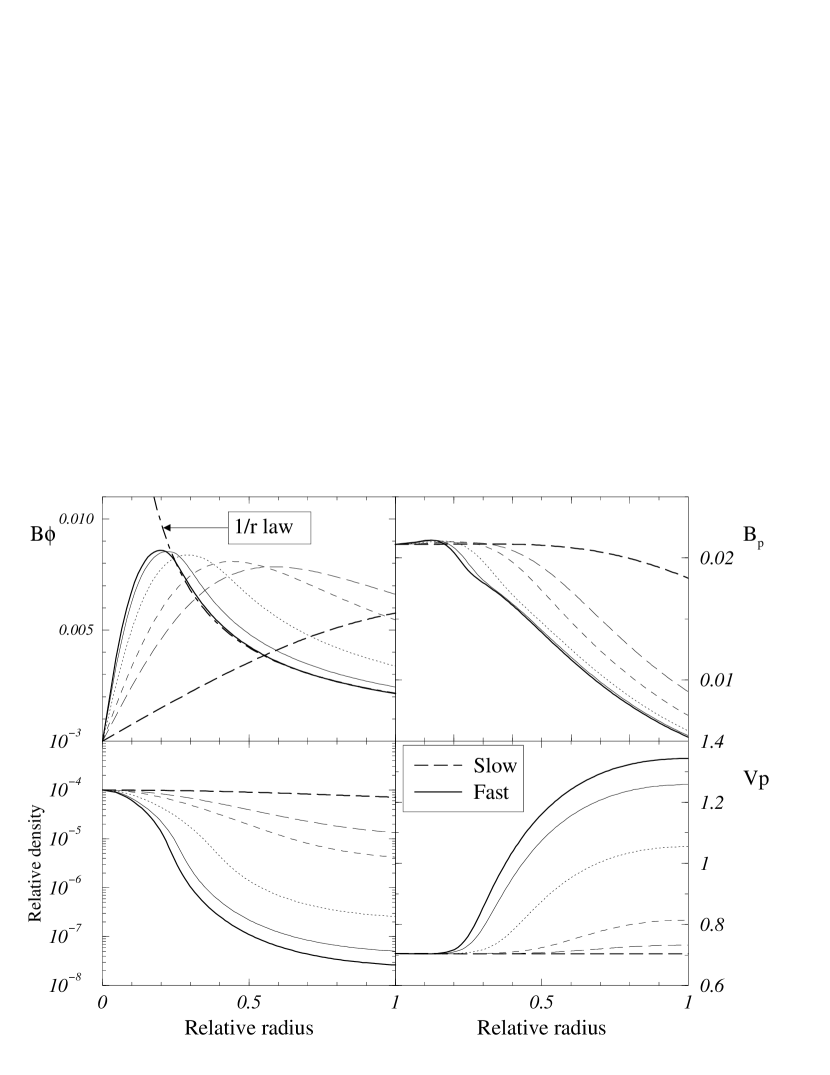
Figure 2: Rotational Effects: The azimuthal $B_{\phi}$ and poloidal $B_{P}$ magnetic field components (upper left and right panels respectively), density $\rho$ and poloidal velocity $v_{\rm P}$ (lower left and right panels) are plotted as functions of relative radius $r_{\rm rel}$ for different values of $\bar{\Omega}$ ($\bar{\Omega}=2$(dashed lines),$4,6,8,10,11$(solid lines)). The corresponding values of $\omega$ are 0.4,1.1,1.3,1.65,1.75 and 1.8. ($\bar{Q}=2.1$ and $\bar{\alpha}_{0}=1.7$)

As in paper I, we find that the variations of the angular velocity have major effects on solutions as can be seen on Fig. 2 that shows the components of the magnetic field, the density and the poloidal velocity for different rotation rates. $\bar{\Omega}$ varies from $2$ to $11$ ($Q_{\ast}=2.1$, $\bar{\alpha}_{0}=1.7$). For a slow rotator (heavy dashed lines in Fig. 2), the toroidal field increases nearly linearly, while it possesses a maximum within the jet for fast rotators. We find that $B_{\phi}\propto 1/r$ while $B_{p}\propto 1/r^{2}$. The two solutions respectively corresponds to a diffuse current with nearly constant current density, and to a centrally peaked current, surrounded by a current-free envelope. A similar behavior has been discussed by Appl & Camenzind (applcam (1993)) for relativistic jets, according to which the jet configurations had been referred to as diffuse and sharp pinch. Important variations with respect to rotation can also be seen in the other physical quantities. In particular the poloidal velocity is highest in the envelope, though variations remain within a factor of two. In the very fast rotator limit the density falls off dramatically in the envelope where the gas pressure becomes negligible compared to the magnetic pressure. This is clearly shown in Fig. 3 where the total pressure is represented with magnetic and gas pressures.

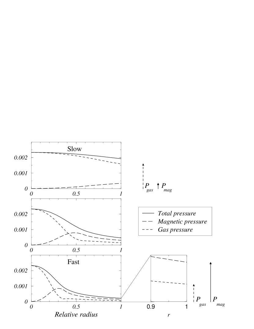
Figure 3: Rotational Effects: Comparison of pressure profiles for slow, fast and very fast rotators. Total, magnetic ($P_{mag}$) and gas ($P_{gas}$) pressure respectively correspond to solid, dashed and long dashed lines. The rotation parameter $\omega$ is equal to 0.4, 1.3 and 1.8 top to bottom respectively.

For slow rotators, the gas pressure dominates everywhere in the outflow, while for fast rotators the magnetic pressure dominates in the envelope. In the latter case, most of the outer pressure at the outer edge is supported by magnetic field and not by gas pressure.

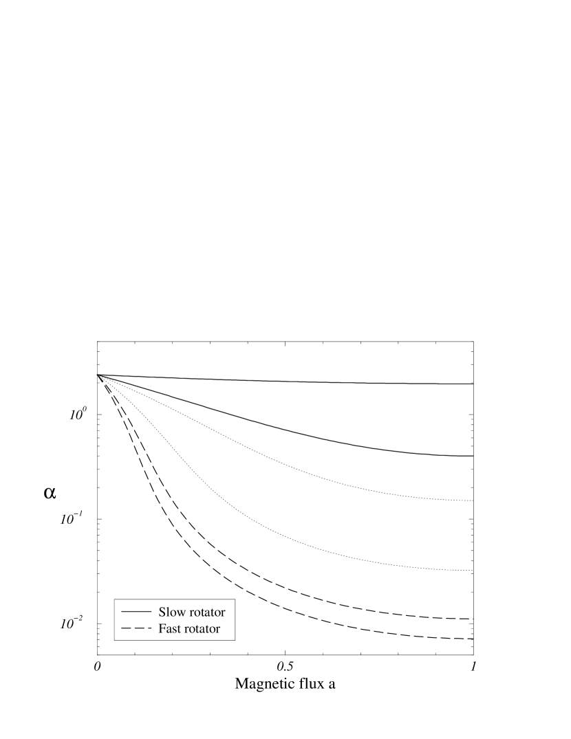
Figure 4: Rotational Effects: Plot of the mass to magnetic flux ratio $\bar{\alpha}$ with respect to the relative magnetic flux $a_{*}=\frac{a}{A}$ for various constant rotation rates $\bar{\Omega}=2..11$. Solid lines correspond to slow rotators, and long dashed lines to outflows with large $\bar{\Omega}$. All the other parameters and boundary conditions are kept the same.

In Fig. 4, the mass to magnetic flux ratio $\bar{\alpha}$ is represented as a function of the relative magnetic flux for various angular velocities. Since the central part of the outflow is denser for fast rotators, the mass flux is very large in this region and very concentrated around the axis. It means that most of the matter is flowing along the polar axis for fast rotators.

3.3 Mass Loss Rate Effects

Figure 5: Mass Loss Rate Effects: Plots of poloidal components of velocity $v_{p}$ (left panel) and magnetic field $B_{p}$ (right panel) for various values of the mass to magnetic flux ratio on the axis $\bar{\alpha}_{0}$. Heavy solid line correspond to small mass loss rates and heavy dashed line to large ones. ($\bar{\alpha}_{0}=0.7,0.8,1,1.4,1.8,2.6$, $\bar{\Omega}=5$ and $\bar{Q}=2.5$)

Another potentially observable quantity is the mass loss rate particularly interesting since it can be evaluated from observations. The parameter related to the mass loss rate is $\bar{\alpha}_{0}$. We have computed solutions for different $\bar{\alpha}_{0}$’s, keeping other parameters unchanged. The results are plotted in Fig. 5 where the poloidal components of the velocity $v_{p}$ and the magnetic field $B_{p}$ are represented as functions of the relative radius. The input values are $\bar{\alpha}_{0}=0.7,0.8,1,1.4,1.8,2.6$, $\bar{\Omega}=5$ and $\bar{Q}=2.5$. From this figure we can infer that the maximum momentum is situated in the axial part, especially for fast rotators. Therefore the central part of the jet will propagate more easily in the ambient medium than the external part.

When the mass loss rate grows, the outflow is slowed down on the edge and accelerated on the axis, while the poloidal magnetic field is also reduced. Therefore the jets from the youngest stellar objects, which show the largest mass loss rates, should have a faster central core and a slower envelope than older ones.

The profile of poloidal velocity depends sensitively on $\bar{\alpha}_{0}$ as well as the core radius that reduces as $\bar{\alpha}_{0}$ increases. As found in Paper I for the inner conical region, it appears that an increase in mass loss rate has a similar effect to a decrease of the rotation rate.

3.4 Thermal Effects

In this subsection we study the dependence of the outflow properties on specific entropy $Q_{\ast}$ on the stellar surface and polytropic index $\gamma$. The other parameters are given by $\bar{\Omega}=\Omega_{\ast}=5$, $\bar{\alpha}_{0}=2.1$ and $\rho_{0}=10^{-5}$. Fig. 6 shows the poloidal velocity $v_{p}$ and the rotation parameter $\omega$ calculated at the outer edge of the flow as functions of the specific entropy $\bar{Q}$. The whole range in $\omega$ can be covered by only varying $\bar{Q}$. Smaller specific entropies correspond to larger $\omega$. For given $\bar{\Omega}$ and $\bar{\alpha}_{0}$ the poloidal velocity presents a minimum when the rotation parameter $\omega$ is almost equal to unity which corresponds to the intermediate class of rotators. Slow rotators are then accelerated by an increase of the heating, but not fast rotators. It has also been found that a change in specific entropy does not affect the azimuthal to poloidal magnetic field ratio but just produces an increase of magnitudes.

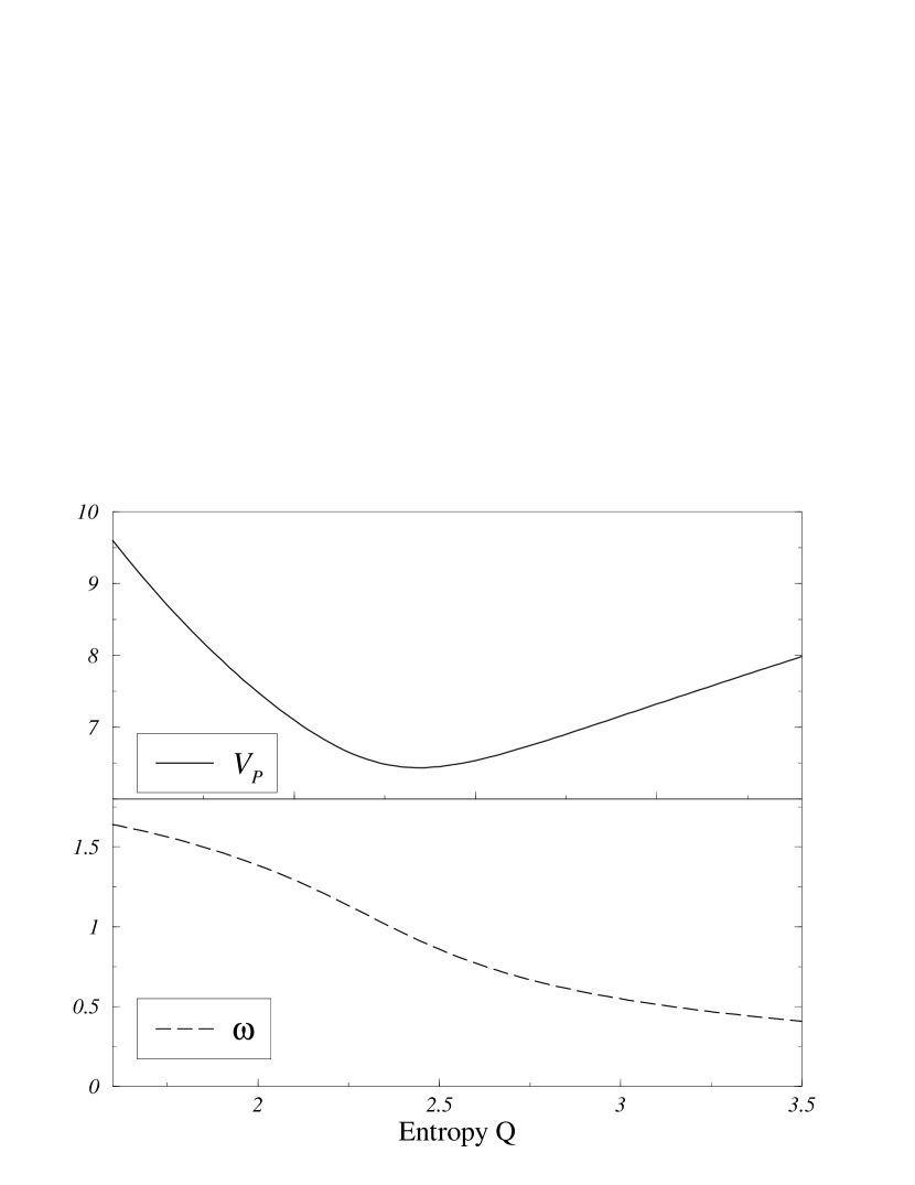
Figure 6: Thermal Effects: Poloidal velocity $v_{p}$ (upper panel) and rotation parameter $\omega$ (lower panel) are plotted for $\bar{Q}$ varying from 1.2 to 3.5 given at the boundary of the outflow. $\omega$ varies from $0$ to its maximum value. $\bar{\Omega}=\Omega_{\ast}=5$, $\bar{\alpha}_{0}=2.1$ and $\rho_{0}=10^{-5}$.

It has been found that the velocity can change by several orders of magnitude, between the adiabatic and isothermal flow, which are the narrower under the same conditions. In Fig. 7, the combined effects of $\bar{Q}$ and $\gamma$ are represented. The rotation parameter $\omega$ is plotted with respect to $\gamma$ for various values of $\bar{Q}$. Two different classes of solutions can be distinguished, solutions for which $\omega$ start at small values for $\gamma=1$ and then decrease and solutions which have large $\omega$ at $\gamma=1$ and then increase. Thus the value of the specific entropy discriminates between fast and slow rotators while larger $\gamma$’s just tighten this distinction.

Figure 7: Thermal Effects: The rotation parameter $\omega$ given at the outer boundary as a function of $\gamma$ for different values of $\bar{Q}$ (from 1 to 3.5) The smallest values of $\bar{Q}$ (represented with solid lines) increase and reach the largest value of $\omega$, while larger value of $\bar{Q}$ (dashed lines) decrease and correspond to smaller values of $\omega$.

3.5 An Example: BP Tau

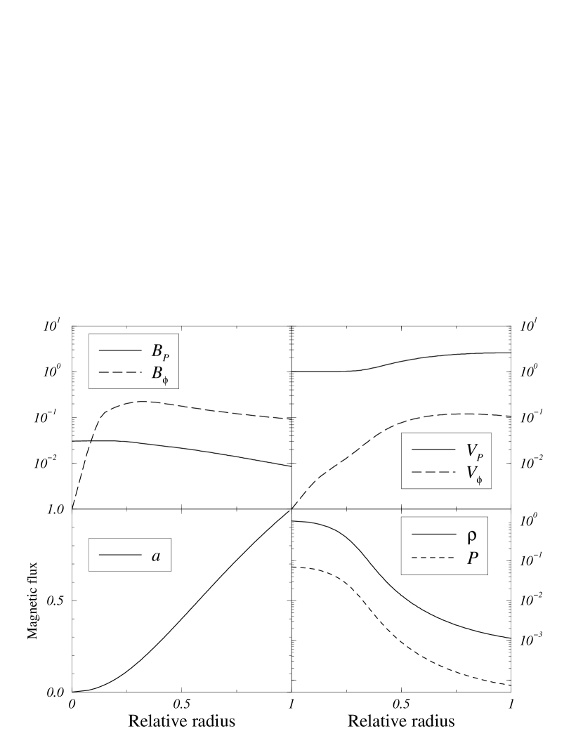
Figure 8: Model for the jet of a TTauri star, BP Tau with $\bar{\Omega}=1.8$, $\bar{\alpha}_{0}=0.1$, $\bar{Q}=0.05$ and a relative central density of $10^{-4}$ ($\omega=1.41$). Upper panels correspond to the magnetic field (left) and the velocity components (right). Density and gas pressure (right) together with the relative magnetic flux (left) are represented in the lowest panels as a function of the relative radius $r_{rel}=r/r_{jet}$.

We now apply the jet model to the TTauri star BP Tau by using its properties, given by Bertout et al.(1988), which are $\dot{M}_{\ast}=2\times 10^{-7}M_{\odot}yr^{-1}$, $M_{\ast}=0.8M_{\odot}$, $R_{\ast}=3R_{\odot}$, $T_{\ast}=9\times 10^{3}$, $n_{p}=10^{4}cm^{-3}$, and $B{\ast}=1000G$. On the base of these values we deduce (see paper I) the corresponding input parameters, which are, expressed in terms of the dimensionless reference values mentioned in section 3.1, $\bar{Q}=0.05$, $\bar{\Omega}=1.8$, $\bar{\alpha_{0}}=0.1$ and a relative central density of $10^{-4}$. These parameters allow to compute the dimensionless rotation parameter $\omega$ which is found to be 1.41 on the equator, and corresponds to the case of a fast rotator. Magnetic field and velocity components, density and gas pressure in the flow are plotted for BP Tau in Fig. 8 together with the magnetic flux represented as a function of the relative radius. The reference units (in CGS) are $\rho_{ref}=70p.cm^{-3}$, $r_{ref}=10^{15}cm$, $v_{ref}=10^{7}cm.s^{-1}$.

The azimuthal component of the magnetic field dominates the poloidal part in the envelope. The poloidal velocity does not show strong variations across the jet, and the azimuthal velocity $v_{\phi}$ is one order of magnitude smaller than the poloidal component. The axial region is the densest and slowest part of the asymptotic flow. This dense core region is a fraction of the full jet with a minimum of $0.5$ for the fastest case. This corresponds to a central core of the order of $5\times 10^{14}cm$. Even if the fastest part is the outer one the maximum momentum is located around the polar axis. Hence even if the relative velocity is smaller close to the axis the central region of the flow will propagate faster in the ambient medium. It also is found that, only in the central part of the asymptotic outflow, does the kinetic energy flux dominate over Poynting flux. Thus a large part of the magnetic energy has not been transferred to the kinetic energy in the case of constant rotation.

3.6 Non-constant $\Omega$ and $Q$

The profiles of the differential angular velocities, that we use (See Paper I), are defined as follows: $\Omega_{0}$ corresponds to a constant rotation rate across the flow, $\Omega_{1}$ is a profile varying from $\Omega_{0}$ to zero with a step-like transition, the same for $\Omega_{3}$ but more smoothly, $\Omega_{2}$ and $\Omega_{5}$ vary from $\Omega_{0}$ to $\Omega_{0}/2$ and $1.5\times\Omega_{0}$ respectively and finally $\Omega_{4}$ follows the differential rotation of a Solar-type star. The profiles of specific entropies are as follows: $Q_{0}$ is constant across the flow, $Q_{1}$ varies from $Q_{0}$ to $Q_{0}/2$ and $Q_{2}$ varies from $Q_{0}$ to zero like $Q_{1}$ but more smoothly in the latter case.

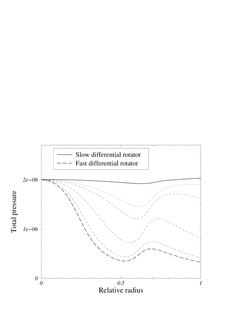
Figure 9: Differential Rotators: we plot the total pressure as a function of the relative radius $r_{rel}$. Slow rotators are represented with solid lines and fast differential rotators with dashed lines. Rotation rate is given by $\Omega_{2}$.

A number of well-collimated outflows are observed to have larger poloidal velocities near the polar axis, and lower velocities at the edge of the flow. This motivated us to use a profile of type $\Omega_{2}$ that could reproduce such behaviors. Fig. 9 represents the total pressure for such differential rotators with respect to the relative radius for a set of central values of the angular velocity. Similarly to rigid rotators, the pressure globally decreases from the axis to the outer edge, though the gradient of rotation causes a second peak of pressure to appear. The latter could correspond to a denser, slower and wider outflow surrounding the central fast jet. For slow and intermediate rotators, the inner pressure can be of order of the pressure at boundary of the outflow and the outer part can be as dense and slow as the axial region. A peak of poloidal velocity accompanies the pressure minimum which produces a double structure in such outflows, with a dense slow core surrounded by a faster component at half of the total radius itself embedded in a slower outer part. Differential rotators can then produce jets with a narrow central part with large momentum surrounded by a larger outflow with smaller momentum, as are jet surrounded by a molecular flow.

It is also found that some outflows like rigid rotators have smaller axial velocities than at the outer edge or present on the contrary a very fast component which corresponds to large gradients of the angular velocity. Differential entropies can also cause such inverted asymptotic solutions though with less amplitude in the variation of the poloidal velocity.

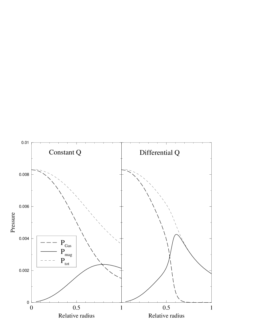
Figure 10: Comparison of the magnetic (solid), the gas (long dashed) and the total (dotted) pressures for constant (left) and differential (right) specific entropies. Parameters correspond to a fast rotator. The angular velocity $\bar{\Omega}$ is constant.

Variations of the entropy profile bring an interesting feature. We have shown previously that magnetic pressure dominates at the outer edge for fast rotators while gas pressure dominates for slow rotators. In fact, variations of the specific entropy enhances this difference as shown in Fig. 10 where the pressures are plotted with respect to the relative radius. The total pressure does not change much as compared to the case of constant entropy while the gas to magnetic pressure ratio $\beta$ decreases. Therefore $\beta$ can become quite low in some regions of the jet. This can have important consequences on the propagation of the jet and on the role of ambipolar diffusion (Frank et al. franketal (1999)) in the dynamics of large scale YSO jets and outflows.

4 The Asymptotic Electric Current

Heyvaerts and Norman (1989) have shown that the asymptotic shape of steady axisymmetric magnetized unconfined outflows is either paraboloidal or cylindrical according to whether the electric current carried at infinity vanishes or not. As shown in previous sections, the uniform confining external pressure causes the flow to asymptote to a cylindrical shape. The aim of this section is to study the variation of the poloidal electric current w.r.t. the confining pressure.

The physical poloidal current through a circle centered on the axis of symmetry and flowing between this axis and a magnetic surface $a$ is given by $I_{phys}(a)=2\pi rB_{\phi}/\mu_{0}$. The related, usually positive quantity $I=-{I_{phys}}/{2\pi}$, which we will still refer to as the ”poloidal electric current” therefore contains entirely equivalent information. The value of the flux surface index, $a$, at the equator corresponds to the total magnetic flux enclosed in the outflow and is defined by $A=\int_{0}^{\pi/2}BR^{2}cos{\theta}d\theta$. We make the magnetic flux dimensionless by dividing it by $A$ and use $a_{*}=a/A$.Let us define the following dimensionless variables normalized to their value at the Alfvén surface, $x\equiv r^{2}/r_{A}^{2}$ and $y\equiv\rho/\rho_{A}$, the thermal parameter $\beta\equiv{2\gamma Q\rho_{A}^{\gamma-1}}/(\gamma-1)v_{PA}^{2}$, the energy parameter $\epsilon\equiv{{2E}/{v_{PA}}^{2}}$, the gravity parameter $g\equiv{{2GM}/{r_{A}v_{PA}}^{2}}$. In terms of these variables the poloidal current can be written, by Eq. (9) which is valid for $r\gg r_{A}$, as

$$I=\frac{A}{\mu_{0}r_{A}}\omega xy$$ (21)

4.1 Current and Pressure Balance

We would like to relate the axial density to the value of the external pressure. It has been found convenient to first consider constant $\Omega(a)$ and $Q(a)$ to investigate the dependence of the electric current on model parameters and on the external confining pressure. Using the dimensionless variables $x$ and $y$ defined above the equations for the asymptotic structure of the flow are written as

$$\left({{dx}\over{da_{*}}}+{\frac{2x}{r_{A}}}{{dr_{A}}\over{da_{*}}}\right)^{2}=\frac{4}{y^{2}\left(\epsilon-\beta y^{\gamma-1}-2\omega^{2}xy\right)}$$ (22)

$$\left(\frac{\gamma-1}{\gamma}\right)xr_{A}^{2}\,\frac{d}{da_{*}}\left(\frac{\beta y^{\gamma}}{r_{A}^{4}}\right)+\frac{d}{da_{*}}\left(\frac{\omega^{2}x^{2}y^{2}}{r_{A}^{2}}\right)=0.$$ (23)

Considering that the variation of the position of the Alfvén point with respect to the relative magnetic flux is small, the Bernoulli equation (22) can be written as

$$\dot{x}={dx\over da_{*}}=\frac{2}{y\sqrt{\epsilon-\beta y^{\gamma-1}-2\omega^{2}xy}}.$$ (24)

Assuming $\Omega(a)$ and $Q(a)$ to be constant, the transfield equation similarly reduces to

$$\dot{y}={dy\over da_{*}}=-y\left({2\omega^{2}\dot{x}}\over{\left(\gamma-1\right)\beta y^{\gamma-2}+2\omega^{2}x}\right).$$ (25)

This equation integrates as

$$\beta y^{\gamma-1}+2\omega^{2}xy=C$$ (26)

where C is an integration constant which can be related to the axial density $y(x=0)=y_{0}$ as

$$C=\beta y_{0}^{\gamma-1}$$ (27)

Using Eq. (26), Eq. (21) becomes

$$I=\frac{A}{2r_{A}\mu_{0}}\frac{\beta}{\omega}\left(y_{0}^{\gamma-1}-y_{b}^{\gamma-1}\right)$$ (28)

where $y_{b}$ is the density at the outer edge. The condition for a vanishing asymptotic current is simply $y_{0}=y_{b}$. In order to relate the latter density to the external pressure, the transfield equation (25) can be reformulated in differential form and, making use of the definition of its integration constant $C$ in Eq. (26), can be cast in the equivalent form

$$\dot{y}=-\frac{2\omega^{2}y^{2}\dot{x}}{\left(\gamma-2\right)\beta y^{\gamma-1}+C}$$ (29)

and the Bernoulli equation is simply

$$\dot{x}=2/y\sqrt{\epsilon-C}$$ (30)

Substituting $\dot{x}$ from Eq. (30) in Eq. (29) we obtain

$$\dot{y}\left(\left(\gamma-2\right)\beta y^{\gamma-2}+C/y\right)=-4\omega^{2}/A\sqrt{\epsilon-C}$$ (31)

that can be integrated between the axis and the outer edge of the outflow ($y$ varies from $y_{0}$ to $y_{b}$ and $\bar{a}$ varies from 0 to 1)

$$C\ln{\left(\frac{y_{b}}{y_{0}}\right)}+\frac{\beta(\gamma-2)}{\gamma-1}\left(y_{b}^{\gamma-1}-y_{0}^{\gamma-1}\right)=-\frac{4\omega^{2}}{\sqrt{\epsilon-C}}.$$ (32)

Note that for this integration the energy has been considered as almost constant w.r.t. $a$, i.e. it does not vary significantly across the jet. This approximation is justified numerically. Pressure balance at the outer edge of the jet gives a relation between the external pressure and the axial density

$$\tilde{P}_{ext}=\frac{\gamma-1}{\gamma}\beta y_{b}^{\gamma}+\omega^{2}x_{b}y_{b}^{2}+y_{b}^{2}(\epsilon-\beta y_{b}^{\gamma-1}-2\omega^{2}x_{b}y_{b})$$ (33)

where $\tilde{P}_{ext}$ is defined by

$$\tilde{P}_{ext}\equiv\frac{2\mu_{0}r_{A}^{4}}{A^{2}}P_{ext}.$$ (34)

Then the pressure balance equilibrium reduces to

$$\tilde{P}_{ext}=\frac{\gamma-1}{\gamma}\beta y_{b}^{\gamma}+\omega^{2}x_{b}y_{b}^{2}+y_{b}^{2}(\epsilon-C)$$ (35)

The system of Eqs. (32) and (33) establishes a relation between the external pressure $\tilde{P}_{ext}$ and the axial density $y_{0}$. Further progress in making it explicit is possible in the case of slow and fast rotators, since simple solutions for $\epsilon$ have been found in paper I.

4.1.1 Slow Rotators

Gas pressure is larger than magnetic pressure at the outer boundary for slow rotators. In this case $\omega\ll 1$, and therefore we have

$$\tilde{P}_{ext}=\frac{\gamma-1}{\gamma}\beta y_{b}^{\gamma}\gg\epsilon-C$$ (36)

The energy parameter $\epsilon$ has been calculated for slow rotators in Paper I and is given by $\epsilon=1+\beta+3\omega^{2}-{\it g}$. Considering $g$ negligible with respect to $\beta$ as a first approximation, Eq. (36) is given by

$$y_{b}=\left(\frac{\gamma\tilde{P}_{ext}}{(\gamma-1)\beta}\right)^{1/\gamma}$$ (37)

Using the definition of $\epsilon$, Eqs. (27) and (37), the Eq. (32) becomes

$$\frac{1}{\gamma}\ln\left(\frac{\gamma\tilde{P}_{ext}}{(\gamma-1)\beta y_{0}^{\gamma}}\right)+\left(\frac{\gamma-2}{\gamma-1}\right)\left(\frac{\gamma\tilde{P}_{ext}}{(\gamma-1)\beta y_{0}^{\gamma}}\right)^{\frac{\gamma-1}{\gamma}}$$

$$=-\frac{4\omega^{2}}{\beta y_{0}^{\gamma-1}\sqrt{1+\omega^{2}-\beta(1+y_{0}^{\gamma-1})}}+\frac{\gamma-2}{\gamma-1}$$ (38)

The second terms of both the left and right hand sides are negligible with respect to the first terms and this equation can be simplified to

$$\tilde{P}_{ext}=\frac{\gamma-1}{\gamma}\beta y_{0}^{\gamma}\exp{-\frac{4\omega^{2}\gamma}{\beta y_{0}^{\gamma-1}\sqrt{1+\omega^{2}-\beta(1+y_{0}^{\gamma-1})}}}$$ (39)

Since $\beta$ and $\omega$ have been obtained by a solution for the inner part of the flow close to the source, this equation is a relation between the external pressure and the asymptotic axial density. It is now possible to calculate the poloidal current as a function of the density on the axis

$$I\approx\frac{\gamma-1}{2\mu_{0}r_{A}}\frac{\beta y_{0}^{\gamma}}{\omega}\left(1-\exp{\left(-\frac{4\omega^{2}\gamma}{\beta y_{0}^{\gamma-1}}\right)}\right)$$ (40)

All other parameters in this formula are given by the solution in the inner part of the flow close to the source and by the boundary condition on the axis. So Eqs. (39) and (40) allow to give a relation between the external pressure and the total poloidal current in the slow rotator case.

4.1.2 Fast Rotators

In this case, the gas pressure is negligible with respect to the magnetic pressure at the outer boundary. This means that

$$\tilde{P}_{ext}=y_{b}^{2}\left(\epsilon-C\right)\ll\epsilon-C$$ (41)

Using Eq. (33) and condition (41), Eq. (32) becomes now

$$\frac{C}{2}\ln\left(\frac{\tilde{P}_{ext}}{\epsilon-C}\right)-\frac{C}{\gamma-1}\ln\left({\frac{C}{\beta}}\right)$$

$$-\frac{\beta(\gamma-2)}{(\gamma-1)}\left(\frac{\tilde{P}_{ext}}{\epsilon-C}\right)^{\frac{\gamma-1}{2}}-\frac{\gamma-2}{\gamma-1}C = -\frac{4\omega^{2}}{\sqrt{\epsilon-C}},$$ (42)

which has two simple solutions, when the external pressure becomes small, which are $C\sim 0$ and $C\sim\epsilon\approx 3\omega^{4\over 3}$. In the latter case the poloidal current is given by

$$I=\frac{A}{2r_{A}\mu_{0}\omega}\left(3\omega^{4/3}-\beta y_{b}^{\gamma-1}\right).$$ (43)

If either $\beta$ or the relative density at the boundary is small compared to unity, it reduces to

$$I=\frac{3}{2}\frac{A}{r_{A}\mu_{0}}\omega^{1/3}$$ (44)

It has been shown in paper I that the Alfvén radius grow with $\omega$ faster than $\omega^{1/3}$ for fast rotators. Then the current decreases as the rotator gets faster. Fast rotators do not carry the largest electric current. When $\omega$ approaches its limit $\left(\frac{3}{2}\right)^{\frac{3}{2}}$ corresponding to the very fast rotator the current approaches

$$I=\left(\frac{3}{2}\right)^{3/2}\frac{A}{r_{A}\mu_{0}}$$ (45)

Since $r_{A}$ has been found in paper I to be proportional to $\alpha^{-1/3}$, the total current increases with $\alpha$.

4.2 Variation of the Current across the Flow

Differentiating the current as given by Eq. (21) with respect to $a$ we find that

$$\frac{dI}{da_{*}}=\frac{2A\omega}{r_{A}\mu_{0}\sqrt{\epsilon-C}}\left(1+\frac{4}{\gamma}\frac{P_{B_{\phi}}}{P_{gas}}\right)^{-1}$$ (46)

Along the same lines as above, we can study the slow rotator case where the gas pressure dominates and the fast rotator case which has a strong magnetic pressure at the outer edge. In the former case, one finds that

$$\frac{dI}{da_{*}}\sim\frac{2A\omega}{r_{A}\mu_{0}\sqrt{1+3\omega^{2}-\beta-\beta y_{0}^{\gamma-1}}}$$ (47)

The slope of the variation of the poloidal current tends to vanish as $\omega$ decreases. It is proportional to $\frac{\omega}{r_{A}}$. For slow rotators the derivative is always positive and then the current is diffuse in the outflow. For fast rotators, $C=\beta y_{0}^{\gamma-1}\ll\epsilon$ and one has

$$\frac{dI}{da_{*}}\sim\frac{A\omega^{1/3}\gamma}{2\sqrt{3}r_{A}\mu_{0}}\frac{P_{gas}}{P_{B_{\phi}}}$$ (48)

The magnitude of the slope $\frac{dI}{da_{*}}$ tends to vanish for very fast rotators since the gas to magnetic pressure ratio decreases with the rotation parameter. In the latter case the slope approaches small values more rapidly than in the slow rotator case. Another interesting point is that the gas to magnetic pressure ratio starts to decrease very rapidly at a small value of the distance $r$ to the axis, so its derivative goes rapidly to zero across the jet as a function of radius. This means that all the current must be enclosed in a core around the axis for fast rotators, which should carry concentrated electric current. Thus it has been found analytically that slow rotators have a diffuse current while fast rotators carry concentrated electric current around the axis.

4.3 Evolution of the Current along the Flow

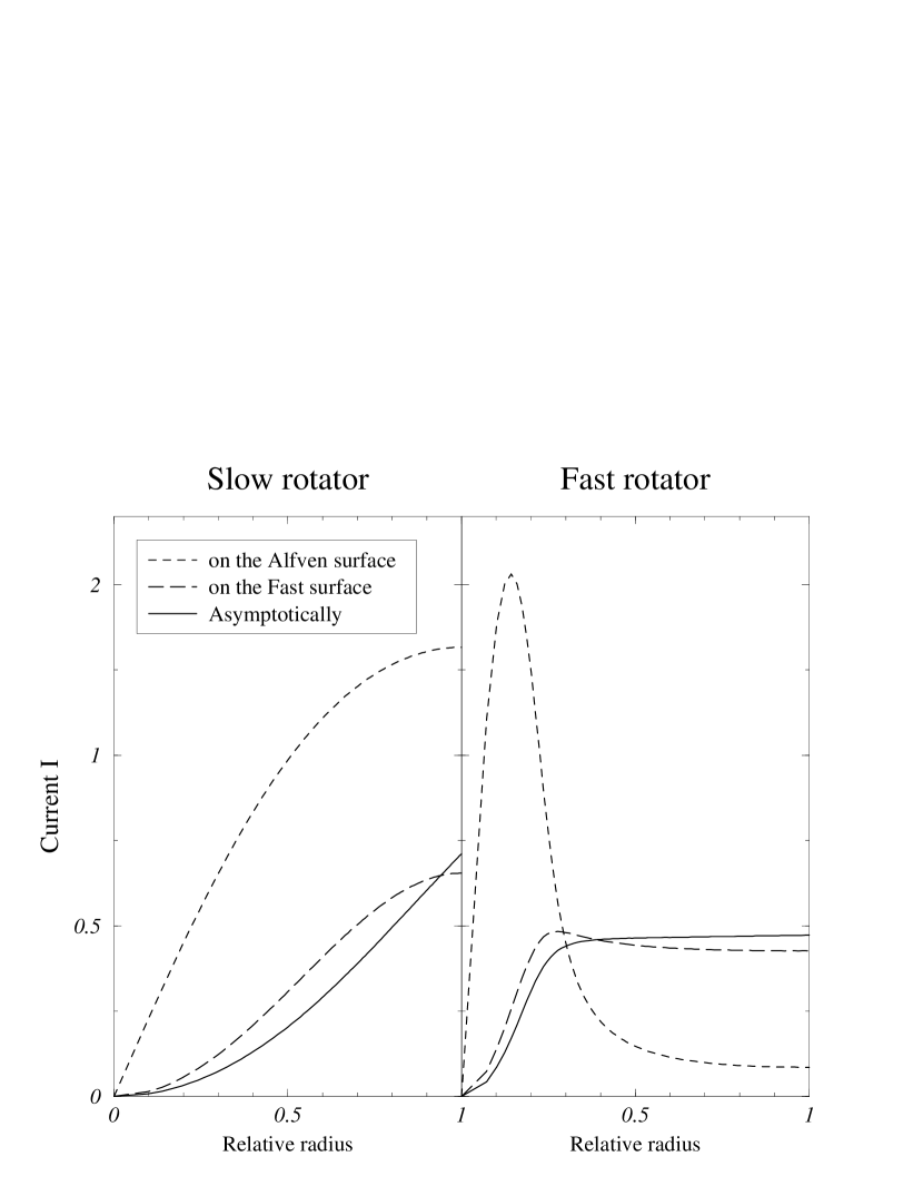
Figure 11: Variations of the current along the flow for slow (left panel) and fast (right panel) rotators as functions of the relative radius. The electric current is calculated in the asymptotic region (solid lines), at the Alfvèn surface (dashed lines) and at the fast magnetosonic surface (long dashed lines).

The variation of the current along one field line gives us fruitful informations on the structure of the outflow and on how the various quantities evolve from the source to infinity. In Fig. 11, the currents calculated at the Alfvén surface, at the fast surface and asymptotically are plotted with respect to the relative radius, which is almost linearly related to $a_{*}={a}/A$ with a slope equal to unity. For slow rotators, the poloidal electric current globally decreases from the Alfvén surface to the asymptotic zone, but is constantly increasing from the polar axis to the edge of the jet. On the other hand the right panel shows that the current at the Alfvén surface has a peak close to the polar axis for fast rotators. The current then decreases at larger distances from the axis which reveals the existence of a return electric current flowing around the central electric flow. This illustrates that the solutions obtained with this model carry return currents at other locations than at the polar axis, contrary to self-similar models.

4.4 Influence of Source Properties

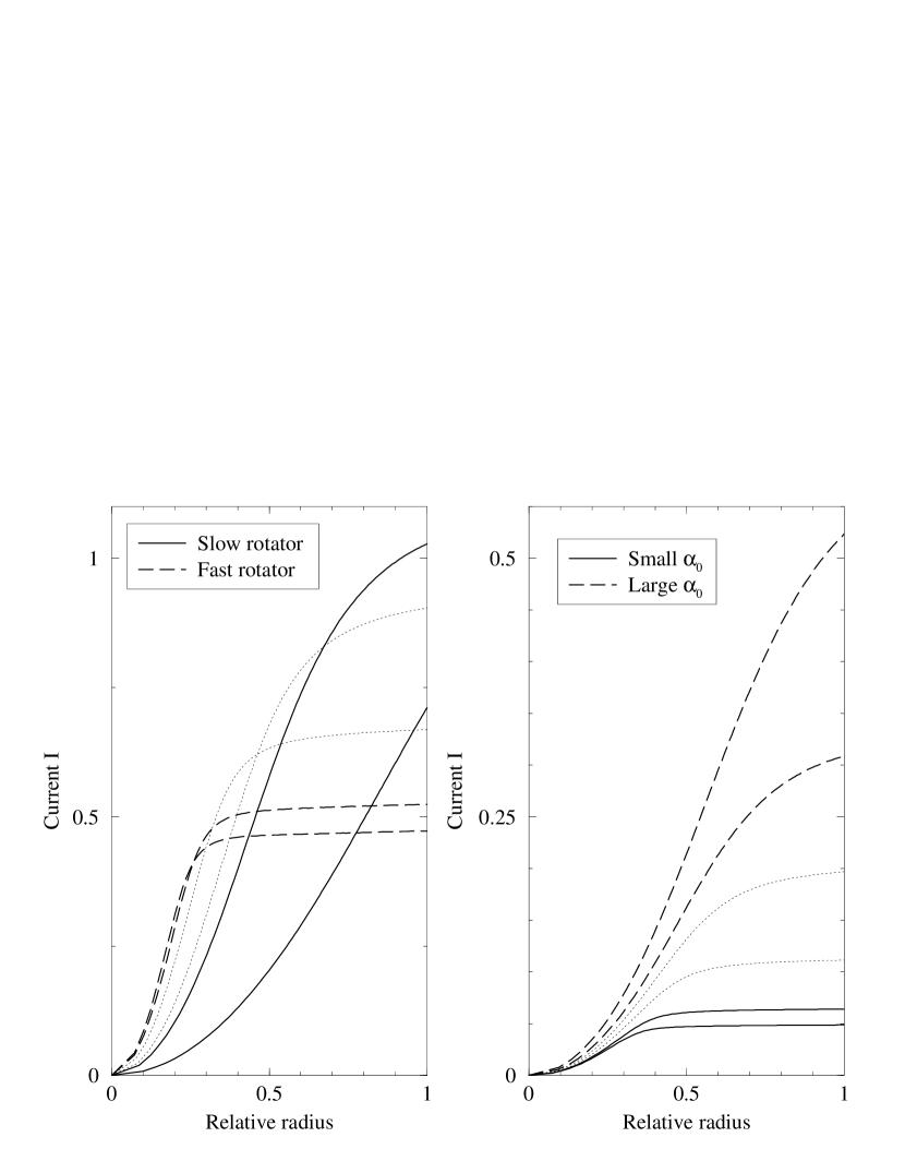
Figure 12: Plots of the asymptotic electric current profile for different values of constant angular velocity $\bar{\Omega}$ (left panel) and of the mass to magnetic flux ratio on the axis $\bar{\alpha}_{0}$ (right panel). Heavy solid lines correspond to slow rotators (left panel) and to small $\bar{\alpha}_{0}$ (right panel), while fast rotators (left panel) and large $\bar{\alpha}_{0}$ are plotted with heavy long dashed lines. Thin dashed lines correspond to intermediate values.

The parameters whose changes produce the strongest variations of the solutions are the angular velocity $\bar{\Omega}$ and the mass to magnetic flux ratio on the axis $\bar{\alpha}_{0}$. The left panel of Fig. 12 represents the variations of the asymptotic poloidal current with the relative radius for various values of $\bar{\Omega}$. As the rotation increases, the current first increases but soon starts to decrease. Moreover the maximum current does not correspond to the largest rotation rate. On the right panel of Fig. 12, the current is plotted for different values of $\bar{\alpha}_{0}$ for a given $\bar{\Omega}$. The larger the mass to magnetic flux ratio, the more the properties of the outflow resemble those of a slow rotator. The current profile changes from a concentrated one, signature of a fast rotator, to a more diffuse one for the largest $\bar{\alpha}_{0}$. The total current increases at the meantime. So jets with large mass loss rate also possess a large current.

4.5 Influence of the External Pressure

Figure 13: Variations of the asymptotic electric current with the external confining pressure for various types of rigid rotators. The solid lines correspond to the fastest rotators while the dashed lines stand for slow rotators. $\bar{Q}=3.1$, $\bar{\alpha}_{0}=2.5$ and $\bar{\Omega}$ varies from 0.1 to 15 corresponding to $\omega$ varying from 0.1 to 1.8.

We plot in Fig. 13 the total asymptotic poloidal current in the jet as a function of the confining pressure for different types of rotators ranging from slow to very fast ones. All other parameters are kept constant. The external pressure can be reduced until the jet reaches unphysical size. The total current diminishes as the external pressure drops for all types of rotators but never approaches a constant non-vanishing limit for the smallest values of the pressure. The slowest rotator in Fig. 13 shows an effect of pressure threshold. For pressures larger than some threshold value the current is almost constant but it strongly decreases for smaller ones. For very fast rotators the current varies little with external pressure.

It would have been interesting to reach a conclusion on whether the asymptotic poloidal current vanishes or not in the limit of vanishing confining pressures. This issue is important because it distinguishes the different possible asymptotic regimes for unconfined jets (Heyvaerts and Norman, 1989). Fig. 13 does not show any leveling-off of the current $I$ as $logP_{ext}$ approaches $-\infty$. Regardless of the smallness of the limiting values of the pressure that have been reached, this study does not allow to conclude that the current vanishes when the pressure rigorously does. However, from a practical point of view, it appears that a significant residual current remains, even for exceedingly small, but non-vanishing, confining pressure.

4.6 Differential Rotators

We now investigate solutions with large gradients of the angular velocity, i.e. $\dot{\omega}\gg\dot{x}$. Eq. (25) can be written as

$$\left(\gamma-1\right)\beta y^{\gamma-1}\dot{y}+2\omega^{2}xy^{2}\left(\dot{y}/y+\dot{\omega}/\omega\right)=0$$ (49)

In this case the transfield equation can be integrated neglecting the relative derivative of the radius with respect to the relative derivatives of the density and of the rotation parameter. The integral is

$$\frac{\gamma-1}{\gamma}\beta y^{\gamma}+\omega^{2}xy^{2}=\beta y_{0}^{\gamma-1}$$ (50)

Eq. (50) can be transformed using Eq. (21) into an equation for the current, that we will note $I_{diff}$, the solution of which is

$$I_{diff}=\frac{A}{r_{A}\mu_{0}}\frac{\gamma-1}{\gamma}\frac{\beta}{\omega y_{b}}\left(y_{0}^{\gamma-1}-y_{b}^{\gamma-1}\right)$$ (51)

This is different from the solution for the rigid rotator case, that can be noted $I_{rig}$. The relation between them is

$$I_{diff}=\left(\frac{\gamma-1}{\gamma}\right)\frac{2}{y_{b}}I_{rig}$$ (52)

This shows that the total current for differential rotators with large gradients of angular velocity will be larger since the density on the boundary is small compared to unity. This can clearly be seen in the left panel of Fig. 14 where the current is plotted with respect to the radius for different types of differential rotators. The largest values of the current correspond to profiles where the gradients of the angular velocity are positive and are the largest, namely for profiles of type $\Omega_{2}$, where the angular velocity takes half of its value at the middle of the outflow.

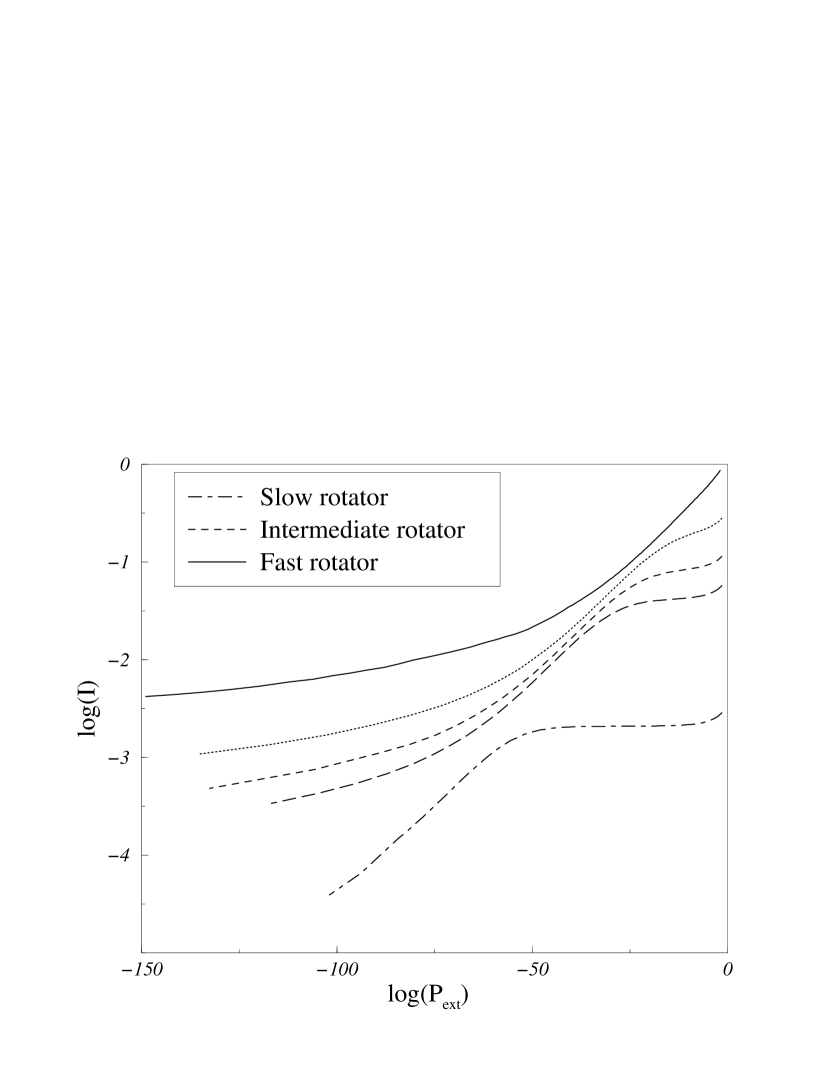
Figure 14: Plots of the electric current profiles across the flow with respect to the relative radius $r_{rel}=\frac{r}{r_{jet}}$. Left panel stands for differential angular velocities and right panel shows differential specific entropies. Note the difference of ranges between different panels.

Fig. 14 shows that the profile of the angular velocity is of prime importance, and that variations of the entropy with flux have a lesser influence on the current profile. Thus jets from differential rotators will carry a larger current and might be more collimated than rigidly rotating outflows.

5 Comparison between Numerical Results and a Simplified Model

In a review of the theory of magnetically accelerated outflows and jets from accretion disks, Spruit (spruit (1994)) discusses the asymptotic wind structure. As in paper I, using his simplifications and method, we find that

$$xy=1-\left(\frac{\alpha}{\alpha_{*}\omega}\right)^{4/3}\left(\frac{r_{A}}{r_{*}}\right)^{2}.$$ (53)

The net current from this simplified analytical model, that we will note $I_{simp}$, is defined by Eq. (21). It is given in the present case by

$$I_{simp}=\frac{9\omega A}{5\mu_{0}r_{*}}\left(\frac{\alpha}{\alpha_{*}}\right)^{1/3}\left(1-\left(\frac{5\alpha}{9\alpha_{*}\omega^{2}}\right)^{2/3}\right)$$ (54)

Thus the current is proportional to the angular velocity and the mass loss rate with the following dependencies

$$I_{simp}\propto\Omega\dot{M}^{1/3}$$ (55)

The current can also be given as a function of the rotation parameter $\omega$ and of the Alfvén radius by

$$I_{simp}\approx 3\omega^{1/3}A/2\mu_{0}r_{A}$$ (56)

We have plotted this analytical solution with respect to $\omega$ in Fig. 15 together with the corresponding numerical solution. As $\omega$ increases and passes $0.5$, the two solutions separate in the intermediate rotator region to converge again in the limit of very fast rotators. As shown previously the current increases with respect to $\omega$ for slow rotators and diminishes in the other limit. So the analytical results we have found for the current are in qualitative agreement with the real value.

Figure 15: Comparison of numerical results (solid line) and analytical solutions (dashed line) of the asymptotic electric current $I$ with respect to the rotation parameter $\omega$.

The Poynting Flux

It is also interesting to calculate the Poynting flux per unit escaping mass which can be written as $S=\Omega rB_{\phi}/\mu_{0}\alpha=I\Omega/\alpha$. Using our dimensionless variables it can be expressed as

$$S=\frac{A^{2}}{\mu_{0}\rho_{A}r_{A}^{4}}\omega^{2}xy=\frac{A}{\rho_{A}r_{A}^{3}}I\omega$$ (57)

Using the previous Eq. (54), the Poynting flux for the above simplified analytical model is given by

$$S_{simp}=\frac{A}{\rho_{A}r_{A}^{3}}\frac{9\omega^{2}A}{5\mu_{0}r_{*}}\left(\frac{\alpha}{\alpha_{*}}\right)^{1/3}\left(1-\left(\frac{5\alpha}{9\alpha_{*}\omega^{2}}\right)^{2/3}\right).$$ (58)

Thus the Poynting flux scales with the rotation and the mass loss rate as

$$S_{simp}\propto\Omega^{2}\ \dot{M}^{-2/3}.$$ (59)

This analytical solution is plotted with respect to the relative radius together with the numerical results with the same input parameters. The agreement is good all across the outflow, and Eq. (58) well reproduces the behavior of the asymptotic Poynting flux. Eq. (58) can be combined with the constraint on the boundary mass density $\rho_{b}$ given in paper I by $\left[S^{2}H\right]_{slow}\geq\left[S^{2}H\right]_{fast}$ where the specific enthalpy $H$ is given at the slow and fast surfaces Thus the asymptotic density at the outer edge of the outflow has an upper bound in terms of quantities defined in the inner part of the outflow close to its source.

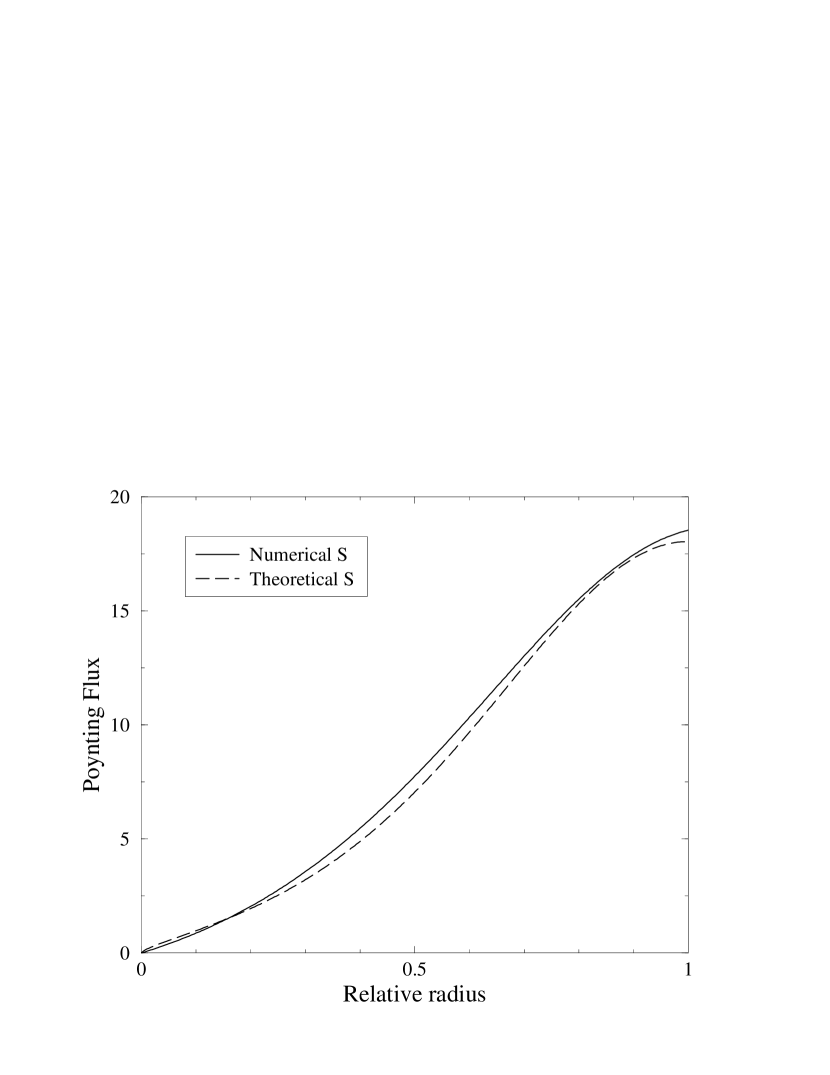
Figure 16: Comparison of numerical results (solid line) and analytical solutions (dashed line) for the Poynting flux $S$ across the outflow as functions of the relative radius $r_{rel}=\frac{r}{r_{jet}}$.

The wind carries both kinetic and magnetic energy, the asymptotic ratio of these, at large distance, is a measure of the importance of the magnetic component. The kinetic energy flux is $K=\rho v_{p}^{2}/2$. The Poynting to kinetic energy flux ratio is given by $q=S/K=3\omega^{4/3}v_{pA}^{2}/\rho v_{p}^{2}$ The effects of the external pressure on the Poynting to kinetic energy fluxes ratio $q$ have been calculated for the different classes of rotators. It is found that the faster the rotator, the larger the ratio $q$ which increases with the confining pressure. Moreover in the asymptotic regime, most of the magnetic energy has been transformed into kinetic energy in the central core close to the axis, contrary to the envelope where $q$ can be very large.

6 Conclusions

We have considered the asymptotic behavior of outflows of magnetized rotators confined by an external uniform pressure in the framework of our simplified model. The asymptotic forms of the transfield and the Bernoulli equations were used to determine the jet structure taking into account the pressure balance across the interface between the flow and the external confining medium. No self-similar assumption has been made. The given confining pressure has been regarded as a boundary condition and the constants of the motion obtained in the inner part of the flow close to the emitting source have been used. The full range of possible variations of the parameters has been explored.

Slow rotators are dominated by thermal effects from the axis to the outer edge. The specific entropy however has little influence on their asymptotic magnetic field. In the case of fast rotators rotational and mass loss rate effects have the most important influences on solutions. Magnetic pressure dominates at the outer edge of the flow. Such rotators asymptotically have a concentrated azimuthal magnetic field $B_{\phi}$, small mass loss rates and large density gradients. A large part of the magnetic energy is not transferred to the kinetic energy and the outflow is asymptotically strongly magnetized and carries a significant Poynting flux.

Whatever the type of rotator, isothermal jets are narrower than adiabatic ones under the same conditions. The densest jets are slower on the boundary than lighter ones. In the case of slow rotators, an analytical solution for the current in terms of the axial density, thermal and rotation parameters has been obtained. This relation combined with the analytical solution gives the asymptotic current as a function of the confining pressure. An analytical solution for the poloidal current has also been obtained in the case of the fast rotator in terms of the rotation parameter and the Alfvén radius. The current in slow rotators is diffuse in the outflow while fast rotators carry a concentrated electric current around the axis. The solutions obtained with our model can carry return currents out of the polar axis, contrary to self-similar models. The comparison between numerical results and approximate analytic solutions show the latter to be good qualitative estimators of the real value.

Non constant profiles of rotation and, to a lesser extent of entropy, cause the solutions to change drastically. For example, the largest asymptotic poloidal velocity can be located either on the axis or at the outer edge according to the profile of $\Omega(a)$. It has been possible to find solutions resembling observed flows such as central jets with important momentum surrounded by a larger outflow. Large currents can be generated by differential rotators if the gradient of the angular velocity is large and the angular velocity does not vanish on the outer edge of the flow.

Thus our model makes it possible to relate the properties of the asymptotic part of an outflow to those of the source. These asymptotic equilibria can be used as input solutions for numerical simulations in order to investigate the propagation of jets and the instabilities that can develop in magnetized outflows.

- (1) Appl S., Camenzind C., 1993, A&A 274, 699
- (2) Bertout, C., et al., 1988, ApJ, 330, 350
- (3) Blandford, R.D., Payne, D.G., 1982, MNRAS, 199, 883
- (4) Chan, K.L., Henriksen, R.N., 1980, ApJ, 241, 534
- (5) Contopoulos, J., Lovelace, R.V.E., 1994, ApJ, 429, 139
- (6) Ferreira, J., Pelletier, G., 1993a, A&A, 276, 625
- (7) Ferreira, J., Pelletier, G., 1993b, A&A, 276, 637
- (8) Ferreira, J., 1997, A&A, 319, 340
- (9) Fiege, J.D., Henriksen, R.N., 1996, MNRAS, 281, 1038
- (10) Frank, A., Mellema, G., 1996, ApJ, 472, 684
- (11) Frank, A., Gardiner, T., Delemarter, G., Lery, T., Betti R., 1999, ApJ, in press
- (12) Goodson, A., Winglee, R., Boehm, K., 1997, ApJ, 489, 199
- (13) Henriksen, R.N., Valls-Gabaud, D., 1994, MNRAS, 266, 681
- (14) Heyvaerts, J., Norman, C., 1989, ApJ, 347, 1055
- (15) Heyvaerts, J., 1996, Plasma Astrophysics eds. Chiuderi, C., Einaudi, G., (Springer), 31
- (16) Lery, T., Heyvaerts, J., Appl, S., Norman, C.A., 1998, A&A, 337, 603
- (17) Lery, T., Henriksen, R.N., Fiege, J.D., 1999, A&A, in press
- (18) Li, Z. Y., Chiueh, T., Begelman, M.C., 1992, ApJ, 394, 459
- (19) Li, Z. Y., 1995, ApJ, 444, 848
- (20) MacGregor, K., B., 1996, in Solar and Astrophysical MHD flows, K. Tsinganos (ed.), Kluwer Academic Publishers, 301
- (21) Ostriker, E.C., 1997, ApJ, 486, 291
- (22) Ouyed, R., Pudritz, R.,1997, ApJ, 482, 712
- (23) Pelletier, G., Pudritz, R.E., 1992, ApJ, 394, 117
- (24) Sauty, C., Tsinganos, K., 1994, A&A, 287, 893
- (25) Shu, F.H., Lizano, S. Ruden, S.P. and Najita, J. 1988, ApJ, 328, L19
- (26) Shu, F.H., Najita, J., Ostriker, E., Wilkin, F., Ruden, S. and Lizano, S., 1994, ApJ, 429, 781
- (27) Shu, F.H., Najita, J., Ostriker, Shang, H., 1997, ApJ, 455, L155
- (28) Spruit, H.C., 1994, Cosmical Magnetism, NATO ASI Series C. eds. D. Lynden-Bell (Kluwer), 422, 33
- (29) Trussoni, E., Tsinganos, K., Sauty, C., 1997, A&A, 325,1099
- (30) Tsinganos, K., Sauty, C., 1992, A&A, 255, 405
- (31) Tsinganos, K., Trussoni, E., 1991, A&A, 249, 156
- (32) Tsinganos, K., Sauty, C., Surlantzis, G., Trussoni, E., Contopoulos, J., 1996, in Solar and Astrophysical MHD flows, K. Tsinganos (ed.), Kluwer Academic Publishers, 379
- (33) Weber, E.J., Davis, L., 1967, ApJ, 148, 217