The ESO Slice Project (ESP) Galaxy Redshift Survey

Abstract

We present analyses of the two-point correlation properties of the ESO Slice Project (ESP) galaxy redshift survey, both in redshift and real space. From the redshift–space correlation function $\xi(s)$ we are able to trace positive clustering out to separations as large as $50\rm\,h^{-1}\,Mpc$, after which $\xi(s)$ smoothly breaks down, crossing the zero value between 60 and $80\rm\,h^{-1}\,Mpc$. This is best seen from the whole magnitude–limited redshift catalogue, using the $J_{3}$ minimum–variance weighting estimator. $\xi(s)$ is reasonably well described by a shallow power law with $\gamma\sim 1.5$ between 3 and $50\rm\,h^{-1}\,Mpc$, while on smaller scales ($0.2-2\rm\,h^{-1}\,Mpc$) it has a shallower slope ($\gamma\sim 1$). This flattening is shown to be mostly due to the redshift–space damping produced by virialized structures, and is less evident when volume–limited samples of the survey are analysed.

We examine the full effect of redshift–space distortions by computing the two–dimensional correlation function $\xi(r_{p},\pi)$ , from which we project out the real–space $\xi(r)$ below $10\rm\,h^{-1}\,Mpc$. This function is well described by a power–law model $(r/r_{o})^{-\gamma}$, with $r_{o}=4.15^{+0.20}_{-0.21}h^{-1}\,$ Mpc and $\gamma=1.67^{+0.07}_{-0.09}$.

Comparison to other redshift surveys shows a consistent picture in which galaxy clustering remains positive out to separations of $50\rm\,h^{-1}\,Mpc$ or larger, in substantial agreement with the results obtained from angular surveys like the APM and EDSGC. Also the shape of the two–point correlation function is remarkably unanimous among these data sets, in all cases requiring more power above $5\rm\,h^{-1}\,Mpc$ (a ‘shoulder’), than a simple extrapolation of the canonical $\xi(r)$ =$(r/5)^{-1.8}$.

The analysis of $\xi(s)$ for volume–limited subsamples with different luminosity shows evidence of luminosity segregation only for the most luminous sample with $M_{b_{J}}\leq-20.5$. For these galaxies, the amplitude of clustering is on all scales $>4\rm\,h^{-1}\,Mpc$ about a factor of 2 above that of all other subsamples containing less luminous galaxies. When redshift–space distortions are removed through projection of $\xi(r_{p},\pi)$ , however, a weak dependence on luminosity is seen at small separations also at fainter magnitudes, resulting in a growth of $r_{o}$ from $3.45_{-0.30}^{+0.21}\rm\,h^{-1}\,Mpc$ to $5.15_{-0.44}^{+0.39}\rm\,h^{-1}\,Mpc$, when the limiting absolute magnitude of the sample changes from $M=-18.5$ to $M=-20$. This effect is masked in redshift space, as the mean pairwise velocity dispersion experiences a parallel increase, basically erasing the effect of the clustering growth on $\xi(s)$ .

keywords – Cosmology – Large–Scale Structure

1 Introduction

The spatial two-point correlation function, $\xi(r)$ , is probably the most classical statistic used in cosmology for clustering analyses. Since its early applications (e.g. Peebles 1980), obtaining reliable estimates of $\xi(r)$ on large ($>5-10\rm\,h^{-1}\,Mpc$) scales became one of the main statistical motivations for enlarging the available 3D samples through new, wider and deeper redshift surveys. The principal reason for this is that on scales sufficiently large for the fluctuations to be still in the linear clustering regime, the shape of $\xi(r)$ is expected to be preserved during gravitational clustering growth. Comparison of observations with models is therefore simpler, because in this case the theoretical description of clustering does not require the full non-linear gravitational modelling, which is on the contrary necessary at small separations. If we are able to measure accurately $\xi(r)$ [or its Fourier dual, the power spectrum P(k)], on large enough scales, we shall have a measure of the distribution of the initial fluctuation amplitudes. In addition, if the initial density field was described by a Gaussian statistics, this will be all the statistical information we need to completely characterise the initial field itself. One further reason for pushing measures of $\xi(r)$ to larger and larger scales, is the possibility to correctly estimate its zero–point, i.e. the scale on which correlations become negative. This is a specific prediction of any viable model, as it reflects the turnover and peak scale in the power spectrum, fingerprint of the horizon size at the matter–radiation equivalence epoch. Clearly, as much as the weakness of clustering in this regime is a benefit for the theory, it represents a hard challenge for the observations: statistical fluctuations destroy any possibility to detect significant features, such as the zero–point of $\xi(r)$ , if the sample under study does not contain enough objects at comparable separations.

Historically, following the pioneering works of the mid–seventies (see Rood 1988 for a review), the industry of redshift measurements exploded in the eighties, with the completion first of the CfA1 (Davis et al. 1982), then of the Perseus-Pisces (Giovanelli et al. 1986) and CfA2/SSRS2 (Geller & Huchra 1989; da Costa et al. 1994) surveys. These first large surveys (containing several $10^{3}$ redshifts), produced significant advances in the estimation of $\xi(r)$ on small and intermediate scales (e.g. Davis & Peebles 1983, De Lapparent et al. 1988). However, they also showed the existence of structures with dimensions comparable to their depth. This, while on one side giving rise to speculations about the very existence of a transition to homogeneity on large scales (see Guzzo 1997 for a recent review of this problem), explicitly indicated the need for larger redshift samples. In more recent years, there have been a few significant attempts to fulfil this need, as for example the surveys based on the IRAS source catalogues (see e.g. Strauss 1996), the Stromlo–APM survey (Loveday et al. 1992b), and especially the Las Campanas Redshift Survey (LCRS, Shectman et al. 1996). Our contribution along this direction has been the realization of the ESO Slice Project (ESP) galaxy redshift survey, that was completed between 1993 and 1996 (Vettolani et al. 1997, Vettolani et al. 1998, V98 hereafter). The technical aims of the ESP survey were to exploit on one side the availability of new deep photometric galaxy catalogues (in our case the EDSGC, Heydon-Dumbleton et al. (1989)), and on the other the multiplexing performances of fibre spectrographs, as in the specific case of the Optopus fibre coupler available at ESO (Avila et al. 1989). The main scientific goals were to estimate the galaxy luminosity function over a large and homogeneously selected sample with a large dynamic range in magnitudes (see Zucca et al. 1997, paper II hereafter), and to measure the clustering of galaxies over a hopefully fair sample of the Universe. The ESP survey, during about 25 nights of observations, produced a $\sim 85\%$ complete sample of 3342 galaxies with reliable redshift. Its combination of depth and angular extension is paralleled at present only by the Las Campanas Redshift Survey (LCRS, Shectman et al. 1996), which has the advantage of containing a larger number of redshifts. One main difference of the LCRS with respect to the ESP, is that it is selected in the red, which makes comparison with the results presented here particularly interesting. One important advantage of the ESP is that it is a purely magnitude–limited sample, which makes modelling of the selection function easier than in the case of the LCRS, where an additional surface–brightness selection was applied.

In this paper we shall discuss the two-point correlation properties of the ESP survey, both in redshift and in real space. Previous or parallel papers, in addition to that describing the above mentioned $b_{J}$–band luminosity function (Zucca et al. 1997), deal with the scaling properties (Scaramella et al. 1998), the properties of groups (Ramella et al. 1998), and potential biases in the estimate of galaxy redshifts (Cappi et al. 1998). The survey in general is described in Vettolani et al. (1997), while the redshift data catalogue is presented in V98. Here we also marginally discuss the small–scale galaxy dynamics, for its effects on redshift–space clustering. However, a proper discussion of the small–scale pairwise velocity dispersion and related topics, will be presented in a separate paper (Guzzo et al. , in preparation).

The paper is organized as follows. Section 2 briefly summarises the properties of the redshift catalogue. Section 3 discusses the techniques used to estimate two–point correlations and their errors. Sections 4 and 5 present the redshift– and real–space correlation functions, discussing their dependence on luminosity and comparing results with other surveys. In section 6 possible biases deriving from the observational setup are investigated. The main results are summarised in section 7.

2 The Survey

The ESP redshift survey consists of a strip of sky $1^{o}$ thick (declination) by $22^{o}$ long (right ascension) near the South Galactic Pole, plus an additional strip of length $5^{o}$ situated five degrees to the west of the main strip. In total, this covers about 25 square degrees at a mean declination of $-40.25^{o}$ between right ascensions $22^{h}30^{m}$ and $01^{h}20^{m}$. The target galaxies were selected from the Edinburgh–Durham Southern Galaxy Catalogue (EDSGC, Heydon–Dumbleton et al. 1989), which is complete to $b_{J}=20.5$. The angular correlation properties of this catalogue were studied in detail in Collins et al. (1992). The limiting magnitude of the ESP is $b_{J}=19.4$, chosen in order to have the best match of the number of targets to the number of fibres in the field of the multi–object spectrograph Optopus, mounted at the Cassegrain focus of the ESO 3.6 m telescope. More details on the observing strategy and the properties of the spectroscopic data are given in Vettolani et al. (1997), and in V98.

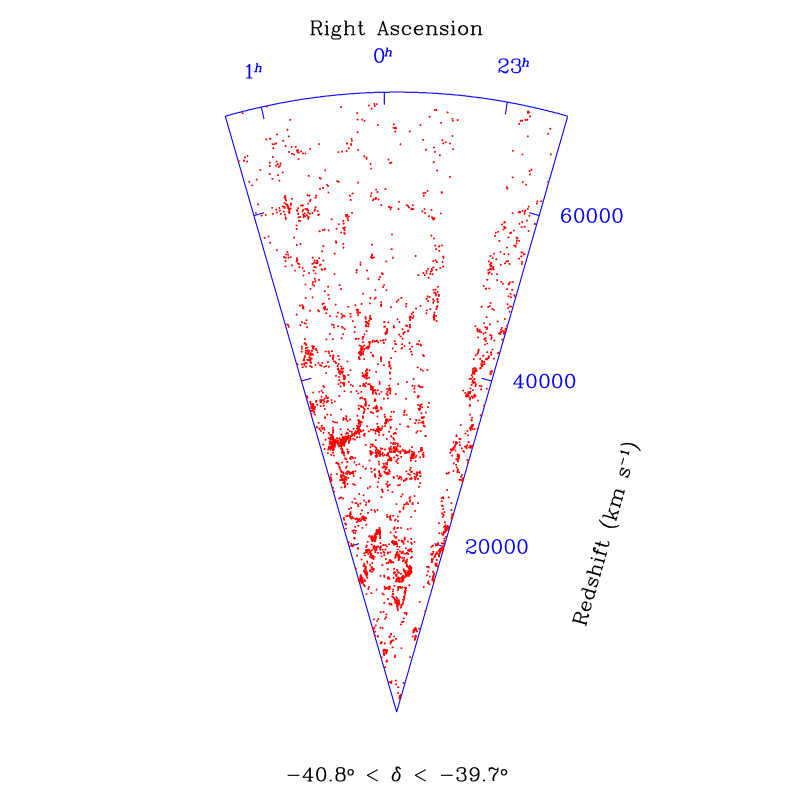
Figure 1: Cone diagram showing the large-scale distribution of galaxies in the ESP survey.

The final galaxy redshift catalogue contains 3342 entries, and is 85% redshift–complete within the survey area. At its effective depth ($z\simeq 0.16$), the transverse linear dimensions of the survey are $\sim 210\rm\,h^{-1}\,Mpc$ by $6.5\rm\,h^{-1}\,Mpc$, while its volume is $\sim 1.9\cdot 10^{5}{\rm\,h^{-3}\,Mpc^{3}}$.

As can be seen in V98, the survey geometry is fairly complex, being composed by two rows of circular Optopus fields, partly overlapping each other. This results in the presence of interstices in which galaxy redshifts were not measured, and which obviously have to be considered carefully in the analysis of clustering. Also, the completeness of each Optopus field is not strictly constant (V98). This will require a weight to be applied to each object, depending on its parent field (see §3.1). The median internal error on the redshift measurements is $64\,{\rm km\,s^{-1}}$ for absorption–line estimates, and $31\,{\rm km\,s^{-1}}$ for emission–line estimates (V98).

In Figure 1 we show a cone diagram of the galaxy distribution in the survey. One first qualitative remark to be made, in view of the use we shall do of the data in this paper, is that the visual impression from this figure suggests - contrary to more ”local” surveys as, e.g. CfA2, a typical size of structures which is smaller than the survey dimensions. This gives us hope that, possibly, clustering measures extracted from this survey would be sufficiently representative of the general properties of our Universe. Clearly, the volume covered by the ESP is still small, due to its limited area coverage on the sky, yet the linear sampling of large-scale structures in two dimensions is unprecedented, and matched only by the even larger LCRS.

Preliminary to the analysis, we performed a series of necessary corrections to the raw data catalogue. We first applied K-corrections to the observed $b_{J}$ apparent magnitudes in the same way as discussed in detail in Zucca et al. (1997). Given the location of the ESP area in the region of the South Galactic Pole, we did not apply any correction for galactic extinction to the observed magnitudes. Observed heliocentric radial velocities were converted to the reference frame of the Local Group using the transformation of Yahil et al. (1977). (We also checked that correcting velocities to the CMB reference frame does not produce any difference in the results). We then computed comoving, luminosity, and angular diameter distances for each galaxy, adopting a cosmological model with H${}_{o}=100$ h $\,{\rm km\,s^{-1}}$ Mpc^-1, and q${}_{o}=0.5$.

The correlation analyses are first performed on the whole apparent–magnitude limited catalogue. To do this, we apply the minimum variance technique (see § 3.1), for which we use the survey selection function as computed in Zucca et al. (1997). We also exclude from this analysis those galaxies lying outside of the range of comoving distances $100\leq D_{com}\leq 500\rm\,h^{-1}\,Mpc$, to avoid using those regions of the sample where respectively either the survey volume or the selection function are dangerously small. The sample trimmed in this way contains 2850 galaxies, with a minimum luminosity corresponding to $M_{b_{J}}=-15.6+5\,{\rm log\,h}$. Using the whole magnitude-limited sample is an attempt to extract the maximum signal from the available data, but can have some drawbacks, as the contribution of galaxies with different luminosities is not homogeneous over the sampled scales.

Therefore, to evidence possible biases and study the general behaviour of clustering with luminosity, we also construct a set of volume–limited subsamples, defined in Table 1. Each column lists, respectively, (1) absolute magnitude limit, (2) luminosity distance computed from the magnitude limit taking into account the K-correction, (3) corresponding comoving distance limit, (4) redshift limit, (5) lower cut in comoving distance, (6) effective volume of the sample between the two distance boundaries, (7) total number of galaxies. Given the small thickness of the ESP slice, the lower distance limits are a safeguard to exclude that part of the samples where galaxy density is potentially undersampled by bright galaxies, thus introducing shot noise. These low cut–off values have been computed as the distance within which, for that absolute magnitude limit, one expects less than 10 galaxies within the corresponding ESP volume, on the basis of the ESP luminosity function. The main analyses we shall discuss in the following are based on the first four samples in the table. These offer the best compromise between having enough volume sampled and a good statistics. However, we also select a more “extreme” sample with $M\leq-20.5$, which contains only 292 galaxies, to study in more detail the existence of luminosity segregation at high luminosities.

$M_{lim}$	$D_{lum(max)}$	$D_{com(max)}$	zmax	$D_{com(min)}$	$Vol$	$N_{gal}$
$-18.5$	328.5	296.8	0.106874	65	$6.109\cdot 10^{4}$	823
$-19.0$	398.7	353.1	0.129082	80	$1.027\cdot 10^{5}$	924
$-19.5$	483.4	418.3	0.155607	100	$1.705\cdot 10^{5}$	819
$-20.0$	590.3	496.6	0.188737	135	$2.834\cdot 10^{5}$	521
$-20.5$	738.4	598.4	0.234030	200	$4.871\cdot 10^{5}$	292

Table 1: Properties of the volume–limited subsamples analysed. Distances (in Mpc), volumes (in Mpc³) and absolute magnitudes ($b_{J}$ system), are computed for h=1, $q_{\circ}=0.5$

3 Computing the Two-Point Correlation Function

3.1 Estimators

There is a long history and literature concerning the theory of statistical estimators of the two–point correlation function $\xi(r)$. The most widely used one (Davis & Peebles 1983), is given by

$$\xi(r)=\frac{2n_{R}}{n_{G}}\frac{GG(r)}{GR(r)}-1\,\,\,\,,$$ (1)

where $n_{G}$ and $n_{R}$ are the mean space densities (or equivalently the total numbers), of objects in the two catalogues, $GG(r)$ represents the number of independent Galaxy-Galaxy pairs with separation between $r$ and $r+dr$, while $GR(r)$ is the number of Galaxy-Random pairs, computed with respect to a random catalogue of points distributed with the same redshift selection function and the same geometry of the real sample (in other words, a Poisson realization of the catalogue). In our case, this implies reproducing the exact distribution of Optopus fields on the sky, and applying the same selection process as done on the real data. One example is the ”drilling” of some areas as it was originally done on the EDSGC around the position of very bright stars (Heydon-Dumbleton et al. (1989)).

The number of $GG(r)$ or $GR(r)$ pairs in eq. 1 can be formed in general including an arbitrary statistical weight, as $GG(r)=\sum_{(i,j)}w_{ij}({r})$, that can depend both on the distances of the two objects from the observer ($d_{i}$ and $d_{j}$), and their separation ($r=|{\bf d_{i}-d_{j}}|$). Here the sum $(i,j)$ extends over all independent pairs with separations between ${r}$ and ${r}+d{r}$. Any weighting which is independent of the local galaxy density will lead to an unbiased estimate of the correlation function, in the sense that the mean value of the estimator, if averaged over an ensemble of similar surveys, would approach the true, underlying galaxy correlation function. However, the variance of individual determinations of $\xi$ around this mean will depend on the particular choice of $w_{ij}(r)$; some choices lead to more accurate estimates than others. By assuming that two–point correlations dominate over higher orders (essentially the linear regime), one finds a useful approximation to the minimum variance weights (Saunders et al. 1992; Hamilton 1993; Fisher et al. 1994a, F94 hereafter), as

$$w_{ij}({r})={1\over 1+4\pi n_{G}\phi(d_{i})J_{3}({r})}\cdot{1\over 1+4\pi n_{G}\phi(d_{j})J_{3}({r})}\,\,\,\,,$$ (2)

where $\phi(d_{i})$ is the survey selection function at the position of galaxy $i$, and $J_{3}({r})\equiv\int_{o}^{r}dr\,r^{2}\xi(r)$. The minimum variance weights themselves, therefore, require knowledge of $\xi$, i.e. we have a circular argument for which one must hope that an iterative procedure would be convergent. We shall instead adopt an à priori model for $\xi$ and use it to calculate the weights; given the host of assumptions employed to arrive at (2), this approach should not be considered as too gross an approximation, as also shown, e.g., by F94. We model $\xi(r)$ as a power law, $\xi(r)=\left({5/r}\right)^{1.8}$ for $r<30\rm\,h^{-1}\,Mpc$, and assume negligible correlations at larger separations. This expression results in ${J_{3}}({r})=15.1\,{r}^{1.2}$, for ${r}\leq 30\rm\,h^{-1}\,Mpc$, and ${J_{3}}=894$ at larger separations.

To test the sensitivity of the results to the adopted model, we also compute ${J_{3}}$ in a different way, i.e. using its definition in terms of the power spectrum P(k). In this case, we have ${J_{3}}({r})\equiv(4\pi r^{3}/3)\int_{0}^{\infty}dkk^{2}P(k)W_{th}(k{r})$, where $W_{th}(kr)$ is the Fourier transform of the spherical top-hat window function. We compute ${J_{3}}$ for the CDM power spectrum normalized to unity in spheres of radius $8\rm\,h^{-1}\,Mpc$. [We note that variants of standard CDM, such as an open model or a low-density flat model with non–zero $\Lambda$, would provide a more realistic power spectrum, but as it is clear from the results of the test, this would make no real difference for our purposes]. We find no significant deviations between the estimates of $\xi(s)$ computed using the two different models for ${J_{3}}$, and therefore used the one based on $\xi(r)$ in the rest of the computations.

The weighting function has to be taken into account also when calculating the mean densities $n_{G}$ and $n_{R}$ to be used in eq. 1. A full discussion of the merits of different estimators for the mean density in a magnitude-limited sample is presented in paper II. In general, an estimate of the mean density, given a weight for each object and the survey selection function, would be of the form

$$n_{G}=\frac{\sum_{i}w_{i}}{\int_{V_{s}}dV\,w(d)\phi(d)}\,\,\,\,,$$ (3)

where the sum extends over all galaxies (or random points), while the integral is extended to the whole survey volume $V_{s}$. In practice, we are interested in the ratio of $n_{R}$ and $n_{G}$, so that we only need to estimate for the two sets of points the value of the quantity in the numerator (i.e. the effective total number of objects). The same arguments leading to eq. (2) result in a similar expression for the minimum variance, single–point weights: $w_{i}=(1+n_{G}\phi(d_{i})J_{3}^{max})^{-1}$ (Davis & Huchra 1982); here $J_{3}^{max}$ is the maximum value of $J_{3}$. Note that again we have one quantity, $n_{G}$, that ideally should be calculated iteratively. However, since in any case our estimator will be unbiased, no matter the choice of the weight, we use here - and correspondingly in the pair weighting - the mean density as estimated in paper II from this same sample, with the same $M_{b_{J}}\leq-12.4+5\,{\rm log\,h}$ cut.

In our specific case, there is an additional complication arising from the varying sampling of the individual Optopus fields, as discussed in § 2. This requires the introduction of another weight, $W^{i}$, to correct for the missed galaxies in each field. Following the same reasoning as detailed in V98, we define the completeness in each field $C^{i}$ as

$$C^{i}={{N^{i}_{Z}}\over{(1-f_{*})\,N^{i}_{T}}},$$ (4)

where $N^{i}_{Z}$ and $N^{i}_{T}$ are the number of secured galaxy redshifts and the number of objects classified as galaxies in the parent photometric catalogue, respectively, in each field $i$, while $f_{*}=0.122$ is the observed fraction of misclassified stars. We therefore multiply the $w_{i}$ corresponding to each galaxy by the weight pertaining to its field, that will be given by $W^{i}=1/C^{i}$ . This is not necessary for the random sample, that, by construction, is uniform over the Optopus fields.

Eq. (1), is based on the definition of $\xi$ (e.g. Peebles 1980), in which it is understood that $n_{G}$ represents the universal mean galaxy density. Any sample mean density will vary about this value with a dispersion at least as large as expected from simple Poisson statistics and, in fact, clustering on the scale of the survey volume will increase this dispersion. The precision of the estimate of $\xi$ at small values (large scales) is limited by this uncertainty, $\delta n_{G}$ (the number of points in the random catalog $N_{r}=V\cdot n_{R}$ may always be sufficiently increased to eliminate its density as a source of uncertainty, and this is in fact what we do here by using typically $N_{r}=100,000$). Given that $n_{G}$ appears linearly in estimator (1), one would conclude that the precision on $\xi$ is also linear in $\delta n_{G}$. In fact, this is not correct, as emphasized by Hamilton (1993) and Landy & Szalay (1993), who suggested alternative estimators in which the precision goes as $\delta n_{G}^{2}$, as would seem more appropriate for the second moment of a distribution.

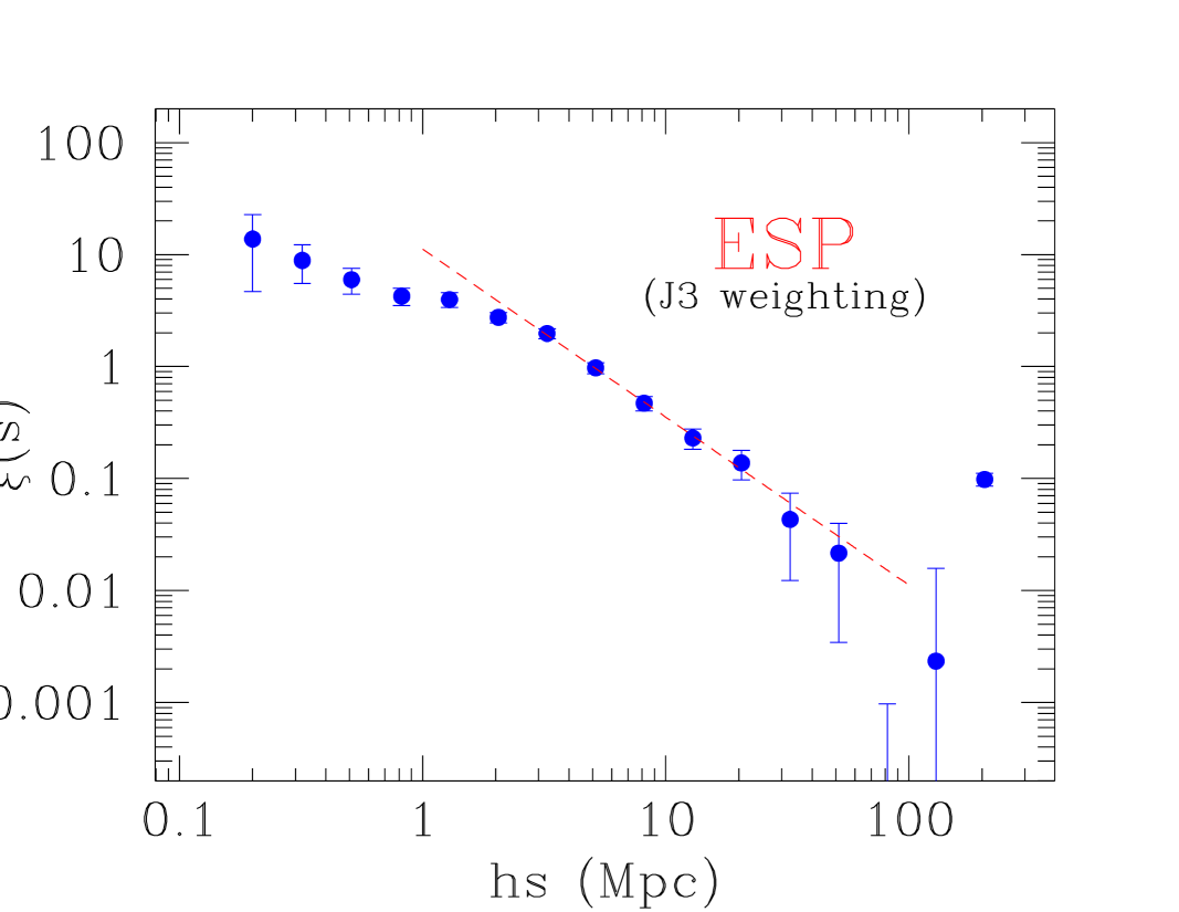
Figure 2: Redshift–space correlation function from the whole ESP magnitude–limited catalogue, computed using the minimum–variance, $J_{3}$–weighting scheme. For reference, the dashed line gives an arbitrary power-law function with $r_{o}=5\rm\,h^{-1}\,Mpc$ and $\gamma=1.5$.

We have computed $\xi(s)$ using (1), and with Hamilton (1993) estimator, and found for our survey equivalent results within the errors. This is partly in contrast to what was found by Loveday et al. on the Stromlo–APM survey (1995), but agrees to the results of Tucker et al. (1997) on the larger LCRS (cf. their Figure 1). The results we shall show in the following are therefore all based on the Davis & Peebles (1983) estimator.

3.2 Error estimation and model fitting

Statistical error bars for our estimates of two-point correlation functions are computed using bootstrap resampling as discussed by Ling et al. (1986). F94 have discussed in detail the reliability of the bootstrap technique in estimating errors for correlation functions; they show that, typically, bootstrap errors are a good description of true rms errors for separations smaller than $\sim 10\rm\,h^{-1}\,Mpc$, while on larger scales they tend to overestimate them by a factor of about 1.5. In the same work, they carefully discuss the technique for fitting of models to correlation functions, where the data points are not statistically independent. We use the same procedure here, which we briefly summarize in the following. Essentially, we create $N_{B}=100$ ”perturbed” realizations of the sample, by randomly sampling the original catalog with replacement, (the ”bootstrapping”). By subjecting each of these realizations to the same analysis, we obtain a set of $N_{B}$ correlation functions: $\xi_{k}(r)$, with $k=1,N_{B}$. We refer to the set of separations $r_{i}$, one for each bin of size $\Delta r$, as separation space. The correlation function $\xi(r)$ is a vector, $\@vec{\xi^{S}}$ in this space with components ${\xi(r_{i})}$. A covariance matrix in separation space may be constructed as

$${\bf C}(r_{i},r_{j})=<(\xi(r_{i})-{\bar{\xi}(r_{i})})(\xi(r_{j})-{\bar{\xi}(r_{j})})>_{realiz},$$ (5)

where ’$<>_{realiz}$’ indicates an average over bootstrap realizations and ${\bar{\xi}(r_{k})}$ is the ensemble average of the correlation function at separation $r_{k}$. Since the values of $\xi$ at two different separations are correlated, ${\bf C}$ is non–diagonal. For this reason one cannot do a straightforward $\chi^{2}$ fit of a model to the observed points. However, ${\bf C}$ is symmetric (${\bf C}=\tilde{\bf C}$) and real, and therefore hermitian, i.e. such that it can be diagonalized by a unitary transformation if its determinant is non–vanishing. What happens in practice, is that the estimated functions are oversampled, so that the effective number of degrees of freedom in the data is smaller than the number of components of $\@vec{\xi^{S}}$. This makes ${\bf C}$ singular, and one has to apply singular value decomposition (as in F94), to recover its eigenvectors. These define the required transformation $T$, to the orthogonal space, i.e. ${\bf C}\rightarrow{\bf D}\ =\tilde{\bf T}\cdot{\bf C}\cdot{\bf T}$ and $\@vec{\xi^{S}}\rightarrow\@vec{\xi^{D}}={\bf T}\cdot\@vec{\xi^{S}}$, where now ${\bf D}$ is diagonal and the components of $\@vec{\xi^{D}}$ are independent. In this space we can therefore define in the usual way the quantity $\chi^{2}$ with respect to our model parameters, and minimize it to find their best–fit values.

4 The Redshift–Space Correlation Function $\xi(s)$

4.1 Optimal weighting

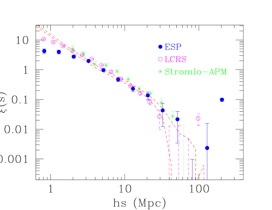
Figure 3: $\xi(s)$ on large scales from the ESP, LCRS (Tucker et al. 1997), and Stromlo–APM (Loveday et al. 1992b), redshift surveys. The dashed lines show the real–space $\xi(r)$ as obtained through deprojection of the angular correlation function for the APM galaxy catalogue, for two clustering evolution models (Baugh 1996).

To maximise the large–scale signal from the data,we first estimate $\xi(s)$ from the whole ESP redshift catalogue, preparred and trimmed as described in § 2. Figure 2 shows the result of applying the $J_{3}$ optimal–weighting estimator to this sample, containing 2850 galaxies. Between 3 and $50\rm\,h^{-1}\,Mpc$ $\xi(s)$ is well described by a shallow ($\gamma\simeq 1.5$) power law, with a redshift–space correlation length $s_{o}\simeq 5\rm\,h^{-1}\,Mpc$. On larger scales, it smoothly breaks down, crossing the zero value between 60 and $80\rm\,h^{-1}\,Mpc$. The bin centered at $80\rm\,h^{-1}\,Mpc$ has indeed a negative value, although it is less than 1$\sigma$ below zero. On larger scales ($r>100\rm\,h^{-1}\,Mpc$), there is marginal evidence that the amplitude of $\xi(s)$ rises up again, a behaviour that seems to be shared also by other clustering data, as we show below. On scales smaller than $3\rm\,h^{-1}\,Mpc$, $\xi(s)$ flattens significantly, so that a single power–law is certainly not a fair description over the whole explored range.

A comprehensive comparison of the best-fit results of a power–law $\xi(s)$ to redshift–space correlation functions from several surveys is given in Willmer et al. (1998). As one could easily guess from our Figure 2, these results are strongly dependent on the range of scales over which the fit is performed, that often is not the same for the different data sets. This makes the comparison of the crude best-fit values rather inconclusive. Equivalently difficult is any physical interpretation of the measured amplitudes and slopes, given that the fit sometimes includes scales where power suppression by virialised structures (“Fingers of God”) is very effective ($s<2\rm\,h^{-1}\,Mpc$), while in other cases it starts above these, putting more weight on less nonlinear scales. Given these ambiguities, here we do not perform a formal fit to the ESP $\xi(s)$ . We shall compute a proper fit only to the real-space correlation function, for which between 0.4 and $10\rm\,h^{-1}\,Mpc$ a power-law shape is a rather good description of the data, and where the observed shape is at least freed of one major distorting effect.

In Figure 3, we compare the $J_{3}$ estimate of $\xi(s)$ from the ESP on large scales to those computed with the same technique from the LCRS and the Stromlo–APM surveys. The agreement between the three estimates is very good between 2 and $30\rm\,h^{-1}\,Mpc$, given also the different galaxy selection functions of the corresponding surveys. On larger scales we can note that the ESP and Stromlo–APM $\xi(s)$ seem to show slightly more power than the LCRS. This evidence for low–amplitude power on large scales, with a smooth decay from the power–law shape, resembles that observed in the IRAS 1.2Jy redshift survey (F94). One could probably explain the differences in Figure 3 with the different selection criteria in the three redshift catalogues: the LCRS is selected in $r$ (with the additional complication of a surface–brightness cut, whose effect is not fully clear), and thus should tend to favour earlier types on the average, that we know reside preferentially in high–density regions. On the other hand, the $b_{J}$ band used for the ESP (so as the IRAS infrared band), is expected to better select star–forming objects in low–density regions. It should probably be expected that ESP galaxies, as well as IRAS galaxies, are better tracers of very large–scale, low–amplitude fluctuations.

In Figure 3, we also plot (dashed lines), the real–space correlation function obtained by deprojecting the angular correlation function $w(\theta)$ from the APM galaxy catalogue (Baugh 1996). This is computed in the case of clustering fixed in comoving coordinates (bottom curve), or growing according to linear theory (top). While the details of the real–space correlation function will be analysed in the following section directly from the ESP itself, here we have the chance to make already a few interesting remarks.

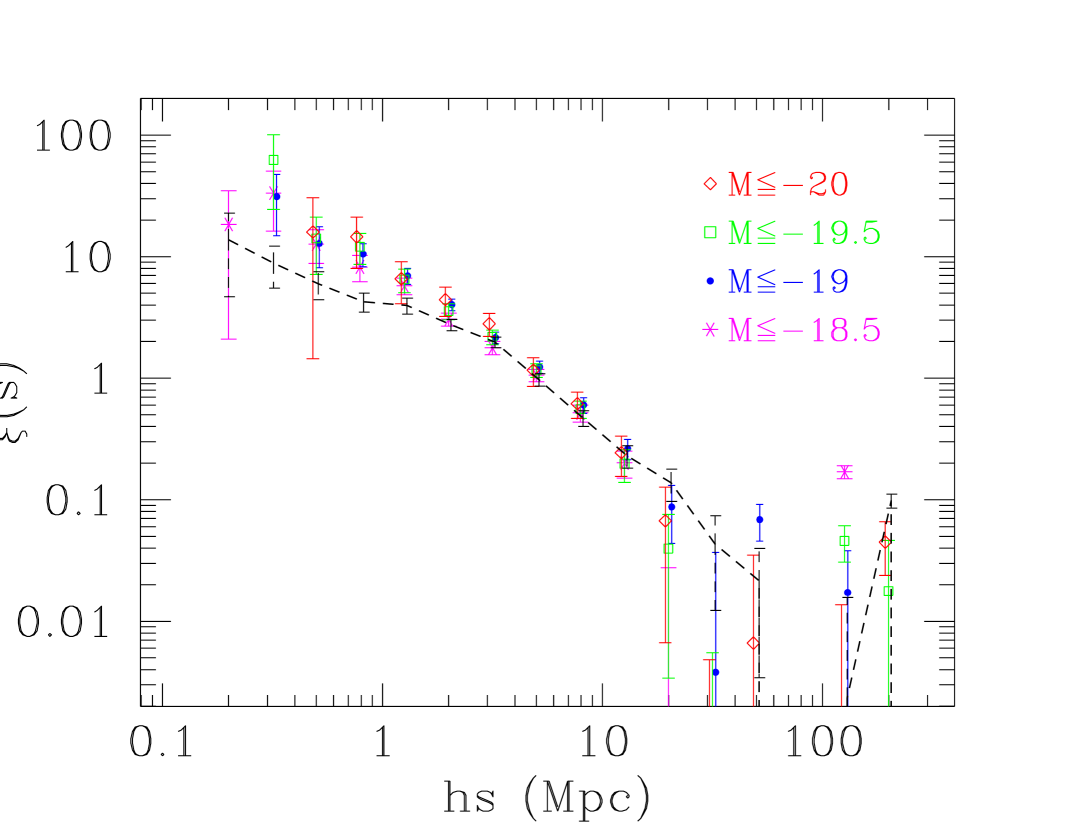
Figure 4: Redshift–space correlation function from four representative volume–limited samples extracted from the ESP as described in Table 1. The dashed line with error bars reproduces the $J_{3}$-weighted estimate from the whole survey. For clarity, points for $M\leq-19$ and $M\leq-20$ are displayed with a shift in log(s).

First of all, the scale of the break in both $\xi(s)$ and $\xi(r)$ is consistently indicated by the different surveys to be between 50 and $90\rm\,h^{-1}\,Mpc$, with the ESP clearly pointing to a value $>50\rm\,h^{-1}\,Mpc$. The agreement between these new redshift data and the APM $\xi(r)$ , directly implies that the large–scale power originally seen in the angular correlation function $w(\theta)$ from the APM (Maddox et al. 1990) and EDSGC (Collins et al. 1992), galaxy catalogues is not significantly enhanced by errors in the magnitude scale, as claimed by some authors (e.g. Bertin & Dennefeld 1997). In fact, Figure 3 demonstrates that similar power is seen in redshift survey data, either based on the same $b_{J}$ plates (ESP) or CCD photometry (LCRS). Also concerning the detailed shape of galaxy correlations above $3\rm\,h^{-1}\,Mpc$, independent data sets show a high degree of unanimity: if one ideally extrapolates to larger scales the ‘classic’ $\sim-1.8$ slope observed in real space below $3\rm\,h^{-1}\,Mpc$ from the APM $\xi(r)$ (but also from previous angular projections, see e.g. Davis & Peebles 1983), all surveys are systematically above this extrapolation. To reproduce this feature (described in the literature as a ‘shoulder’ or a ‘bump’, see Guzzo et al. 1991, and Peacock 1997), a rather steep ($\sim k^{-2}$) power spectrum P(k) is required (Branchini et al. 1994, Peacock 1997).

A second important point about Figure 3 concerns the effect of redshift–space distortions. One can see how small is the amplitude difference between the redshift–space correlation functions and the APM real–space $\xi(r)$ on large scales. A linear amplification is indeed expected as a result of coherent flows towards large–scale structures. This can be approximately expressed as $\sim$ $1+{1\over 2}{\beta}+{1\over 5}{\beta^{2}}$, where $\beta=\Omega_{o}^{0.6}/b$ and $b$ is the linear biasing factor (Kaiser 1987). Figure 3 implies, within the errors, a value for this factor very close to 1. For example, a value of 1.2, consistent with the observed data, would yield $\beta=0.35$.

It is interesting to note that the Stromlo–APM $\xi(s)$ is the only data set that around $\sim 10\rm\,h^{-1}\,Mpc$ seems to show a significant amplification with respect to $\xi(r)$ . (Note that this comparison is actually the safest, being the APM catalogue the parent photometric list of the Stromlo–APM redshift survey). The interpretation of this effect is however complicated by what we have pointed out in Paper II, where we showed how the mean density in this redshift survey is about a factor of 2 lower with respect to that deduced from deeper samples. The cause for this seems to be a negative density fluctuation that we clearly detect in the ESP data below $z<0.05$, and that is also visible in other surveys. This ”local” underdensity, is shown to be the explanation for both the low normalization of the Stromlo–APM luminosity function (Loveday et al. 1992a), and the steep number counts observed at bright magnitudes in several bands (e.g. Maddox et al. 1990). It is not trivial to understand how this systematic 50% underestimate of the mean density would affect the two–point correlation function, although it clearly reduces by the same amount the number of pairs expected at a given separation. If this deficit is evenly spread on all scales, then the measured $\xi(s)$ will be practically unaffected, however if it corresponds, for example, to a region with larger-than-average voids, the net effect will be to boost up $\xi(s)$ by some amount. This would be sufficient to produce the observed discrepancy between $\xi(s)$ and $\xi(r)$ , and further demonstrates how extended and accurate the data have to be in order to extract dynamical information as the value of $\beta$.

4.2 Volume–limited estimates

While the $J_{3}$–weighted estimate has the advantage of maximising the information extracted from the available data, it has some important drawbacks that have been not always appreciated in previous applications. The main problem is that by its own definition it inevitably mixes the contribution of galaxies with different luminosities. This would not be a problem if galaxy clustering were completely independent of luminosity, i.e. if each galaxy traced fluctuations independently from its own absolute magnitude. As we discussed in §3.1, this technique weighs pairs based both on their separation and on their distance from the observer. This implies that the main contribution to small–scale correlations comes from low–luminosity pairs, that are numerous (and dense) in the nearby part of the sample and thus better trace clustering at small separations. On the contrary, the estimate of $\xi(s)$ on large scales is dominated by the contribution from luminous objects, that are in fact the only ones detectable in the distant part of the survey. Clearly, if there is any luminosity dependence of clustering, this technique will tend to modify in some way the shape of $\xi(s)$ . In particular, if luminous galaxies are more clustered than faint ones, the $J_{3}$ weighting will tend to give a shallower slope for a power–law shaped correlation function. Therefore, while this method is certainly optimal for maximising the clustering signal on large scales (and so our conclusions on the large–scale shape of $\xi(s)$ from the previous section should not be affected), it might be dangerous to draw from its results far–reaching conclusions on the global shape of $\xi(s)$ , especially on small scales. A wise way to counter–check the results obtained from the optimal weighting technique, is that of estimating $\xi(s)$ also from volume–limited subsamples extracted from the survey. In this case, each sample includes a narrower range of luminosities and no weighting is required, the density of objects being the same everywhere. This means that in our case $w_{i}({r})\equiv 1$, and only the $W^{i}$’s have to be taken into account.

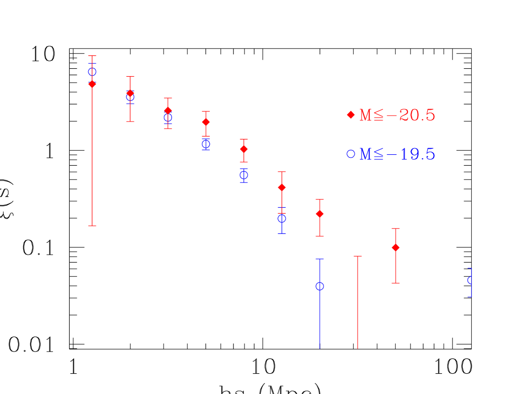
Figure 5: A further test for luminosity dependence of clustering in redshift space. $\xi(s)$ for the brightest ($M\leq-20.5$) volume-limited subsample of the ESP is compared to one of the main samples from the previous figure. Note that the scale has been changed to better evidence the difference in amplitude on intermediate scales.

We have performed this exercise on the ESP, and the results for the four main samples defined in Table 1 are displayed in Fig. 4. In the figure, we also reproduce the $J_{3}$–weighted estimate (dashed line). To ease visualization, the data points for the $M\leq-20$ and $M\leq-19$ samples have been shifted by a constant value (negative and positive respectively) in log$(s)$. It is clear how for the ESP data the $J_{3}$–based method produces a $\xi(s)$ which is shallower below $3\rm\,h^{-1}\,Mpc$. On larger scales the shape is consistent between the two methods, and for $s>20\rm\,h^{-1}\,Mpc$ the optimal weighting performs better in terms of signal–to–noise, than the single volume–limited estimates. The observed $\xi(s)$ is in practice the result of the convolution of the real–space correlation function $\xi(r)$ with the distribution function of pairwise velocities. This means that the small–scale flatter shape of $\xi(s)$ in the case of the magnitude–limited sample could be in principle produced either by a smaller $\xi(r)$ or by a higher pairwise velocity dispersions. We find (Guzzo et al., in preparation), that most of the effect is produced by this second factor: the small–scale pairwise velocity dispersion between 0 and $1\rm\,h^{-1}\,Mpc$, is higher when measured on the whole survey using the $J_{3}$–weighted method. We measure $\sigma_{12}(1)\simeq 600\,{\rm km\,s^{-1}}$ using the ${J_{3}}$ estimate from the whole sample, while the volume–limited samples give values between 300 and $400\,{\rm km\,s^{-1}}$, depending on the infall model adopted.

From this plot alone there is no evident sign of a luminosity dependence of $\xi(s)$ , since the four estimates are virtually the same within the errors. From their analysis of the SSRS2 sample, Benoist et al. (1996), also find that there are negligible signs of luminosity segregation for galaxies fainter than $M^{*}$, which in our case corresponds to $-19.6$. They also show, however, that a clear effect becomes visible for absolute magnitudes brighter than $\sim-20$. To check for this effect in more detail, in Fig. 5 we plot $\xi(s)$ for the brightest sample that can be selected from the ESP while keeping a reasonable statistics, with $M\leq-20.5$. This estimate is compared to that for the $M\leq-19.5\simeq M^{*}$ sample from the previous figure. Here, we see a significant increase in the amplitude of $\xi(s)$ for the more luminous galaxies, for separations above $3-4\rm\,h^{-1}\,Mpc$. Even if we do not perform a formal fit for the reasons discussed above, we see that now $\xi(s)$ passes through unity around $r\sim 8\rm\,h^{-1}\,Mpc$, i.e. has an amplitude very consistent to that observed by Benoist et al. (1996) for galaxies with similar luminosity in the SSRS2.

These authors also point out how the detection of luminosity segregation is complicated by volume effects (different samples covering different volumes), and by redshift–space distortions. For these reasons, the results of Figures 4 and 5 are probably meaningful for what concerns the shape and amplitude of $\xi(s)$ on scales $>4-5\rm\,h^{-1}\,Mpc$ (given also the negligible amount of redshift–space amplification that we have shown in Figure 3). On smaller scales, however, clustering and dynamics mix up in a non–trivial way for the different samples, so that the simple redshift–space correlation function is possibly hiding a large amount of information. Guzzo et al. (1997) have shown how to disentangle some of these effects by studying the differences of clustering in real space in the case of the Persus–Pisces survey. More recently, Willmer et al. (1998) have studied $\xi(r)$ and $\xi(s)$ in the SSRS2 survey for different luminosity subsamples. We shall see in § 5 how also in the case of the ESP, when studying $\xi(r_{p},\pi)$ and its real–space projection $w_{p}(r_{p})$ , it is possible to evidence some weak positive trend of clustering with luminosity also at small separations.

5 $\xi(r_{p},\pi)$ and the Real–Space Correlation Function

So far, we have considered the correlation among galaxies as located in redshift space, where a map of the galaxy distribution is distorted due to the effect of peculiar velocities, whose contribution adds to the Universal expansion to produce the redshift we actually measure. The effect of redshift–space distortions can be shown explicitly through the correlation function $\xi(r_{p},\pi)$ , where the separation vector of a pair of objects is split into two components: $\pi$ and $r_{p}$, respectively parallel and perpendicular to the line of sight. Given two objects with observed radial velocities $v_{1}=cz_{1}$ and $v_{2}=cz_{2}$, following F94 we define the line of sight vector ${\bf l}\equiv({\bf v}_{1}\ +{\bf v}_{2}\ )/2$ and the redshift difference vector ${\bf s}\equiv{\bf v}_{1}\ -{\bf v}_{2}\$, leading to the definitions

$$\pi\equiv{{{\bf s}\cdot{\bf l}}\over{{\rm H_{0}}|{\bf l}|}}\quad\quad r_{p}^{2}\equiv{{\bf s}\cdot{\bf s}\over{\rm H_{0}^{2}}}-\pi^{2}\,.$$ (6)

We can then generalize estimator (1) to the case of $\xi(r_{p},\pi)$ , now counting the number of pairs in a grid of bins $\Delta r_{p}$, $\Delta\pi$.

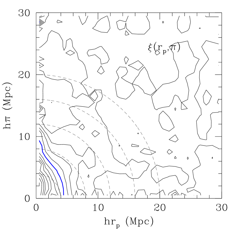
Figure 6: $\xi(r_{p},\pi)$ for the ESP magnitude–limited sample. The heavy contour corresponds to $\xi=1$; for higher values of $\xi$, contours are logarithmically spaced, with $\Delta\log_{10}\xi=0.1$; below $\xi=1$, they are linearly spaced with $\Delta\xi=0.2$ down to $\xi=0$. The dashed contours represent the isotropic correlations expected in the absence of peculiar velocities. The map has been Gaussian-smoothed with an isotropic filter of width 3 $\rm\,h^{-1}\,Mpc$.

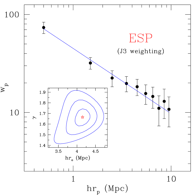
Figure 7: Results of the fit of a power–law $\xi(r)$ to the projected function $w_{p}(r_{p})$ (filled circles), for the whole magnitude-limited redshift sample. The inset shows the corresponding best-fit values for the correlation length $r_{o}$ and the slope $\gamma$, together with the single-parameter confidence contours at the 1-, 2- and 3-$\sigma$ levels.

Figure 6 displays the observed $\xi(r_{p},\pi)$  for the ESP survey, estimated from the magnitude-limited sample using the same minumum weighting technique used for computing $\xi(s)$ , but binned linearly into bins of $1\rm\,h^{-1}\,Mpc$. As expected, the iso–correlation contours of $\xi(r_{p},\pi)$ are stretched along the line of sight ($\pi$) at small separations, with respect to the isotropic case (dashed circular contours). This is the effect of the relative velocity dispersion of galaxy pairs, $\sigma_{12}$, and includes the contribution of both the large velocity dispersion cluster galaxies, and the cooler field population. A careful estimate of $\sigma_{12}$ and a discussion of the small-scale dynamics in the ESP survey will be presented in a separate paper. Here we limit the analysis of $\xi(r_{p},\pi)$ to the task of recovering the real-space correlation function $\xi(r)$ .

The standard way to recover $\xi(r)$ is to project $\xi(r_{p},\pi)$  onto the $r_{p}$ axis, in this way integrating out the dilution produced by the redshift-space distortion field. The resulting quantity is

$$w_{p}(r_{p})\equiv 2\int_{0}^{\infty}dy\,\xi(r_{p},\pi)=2\int_{0}^{\infty}dy\,\xi\left[(r_{p}^{2}+y^{2})^{1/2}\right]\,,$$ (7)

where the second equality follows from the independence of the integral on the redshift-space distortions. In the right-hand side of the equation, $\xi$ is the real–space correlation function, evaluated at $r=(r_{p}^{2}+y^{2})^{1/2}$. With a power-law model for $\xi(r)$, i.e. $\xi(r)=(r/r_{0})^{-\gamma}$ the integral can be computed analytically, yielding

$$w_{p}(r_{p})=r_{p}\left({r_{0}\over r_{p}}\right)^{\gamma}{\Gamma({1\over 2})\,\Gamma({\gamma-1\over 2})\over\Gamma({\gamma\over 2})}$$ (8)

where $\Gamma$ is the Gamma function. The upper integration limit in Eq. (7), $\pi_{up}=\infty$, is chosen in practice so as to be large enough to produce a stable estimate of $w_{p}$. As in previous works (Guzzo et al. 1997), we find $w_{p}(r_{p})$  to be quite insensitive to $\pi_{up}$ in the range $20\rm\,h^{-1}\,Mpc<\pi_{up}<25\rm\,h^{-1}\,Mpc$ for $r_{p}<10\rm\,h^{-1}\,Mpc$. In fact, for small values of $r_{p}$, it is important not to choose a too small upper limit, since this would leave out small-scale power that is present at large $\pi$’s due to the stretching. On the other hand, the choice of too large a value for $\pi_{up}$, has the only effect of adding noise into $w_{p}$.

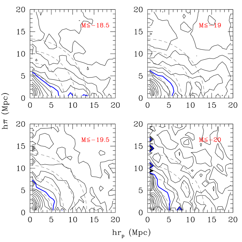
Figure 8: $\xi(r_{p},\pi)$ for the four main volume–limited subsamples of the ESP catalogue. Contour levels are defined as in Figure 6.

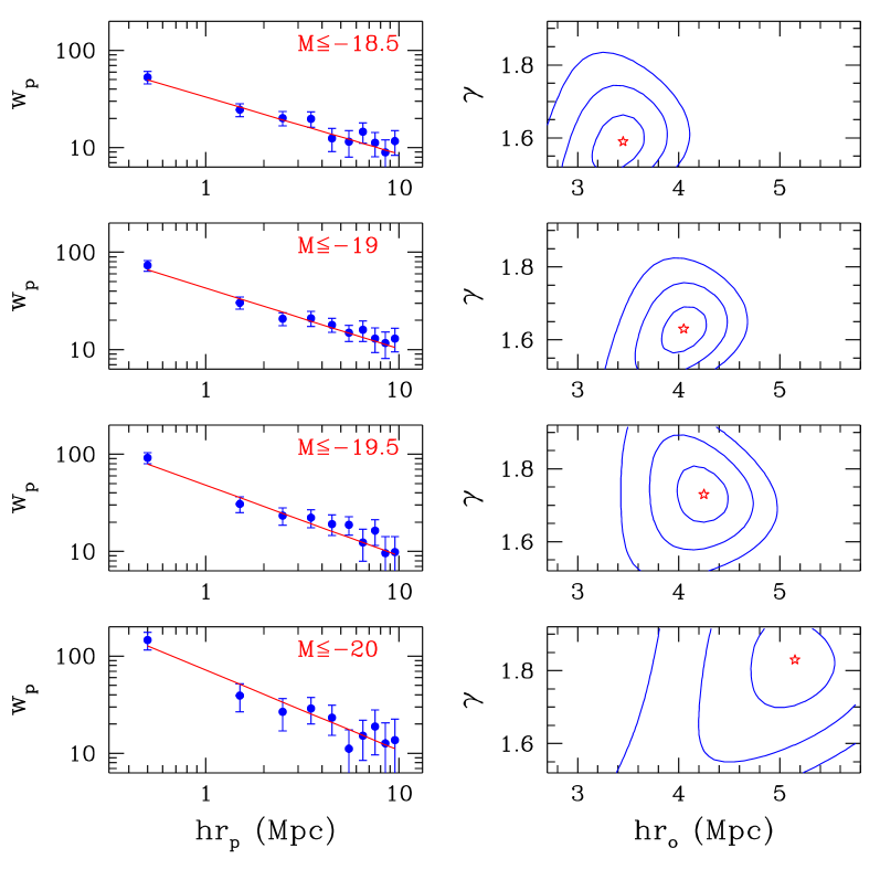
Figure 9: Best–fit results of a power–law $\xi(r)$ to the projected function $w_{p}(r_{p})$ for the same four volume–limited samples of the previous figure. Left panels give the observed $w_{p}(r_{p})$ with the corresponding best-fit power law. Right panels show the best-fit $r_{o}$ and $\gamma$ values, together with their 1-, 2-, and 3-$\sigma$ confidence levels.

The computed $w_{p}(r_{p})$  for the whole magnitude–limited ESP catalogue is shown in Figure 7 (solid circles), together with the results of the fit of a power-law model for $\xi(r)$ (solid line and inset). Error bars are as usual computed over 100 bootstrap realizations of the sample. The corresponding best-fit values are $r_{o}=4.15^{+0.20}_{-0.21}h^{-1}\,$ Mpc and $\gamma=1.67^{+0.07}_{-0.09}$. These values are smaller than those measured from the LCRS, for which Jing & Börner (1996) obtain $r_{o}=5.06\pm 0.12$ and $\gamma=1.862\pm 0.034$. The reason for this difference is probably to be found in the different galaxy populations that these two surveys preferentially select, an effect possibly enhanced by the faint limiting magnitude of the two surveys. In fact, from the blue-selected SSRS2 (limited to $m=15.5$, i.e. 4 magnitudes brighter than the ESP), Willmer et al. (1998) measure a real–space correlation function with $r_{o}=5.36\pm 0.33$ and $\gamma=1.86\pm 0.16$, i.e. virtually identical to the red–selected LCRS. Clearly, given its fainter magnitude limit, in the ESP a much larger population of intrinsically faint, possibly less clustered, galaxies enters the sample. This could well be the reason for the smaller global clustering amplitude measured from the magnitude-limited sample, where, as we explained above, faint nearby galaxies play a dominant role on small scales in the J3–weighted technique.

Let us now look at $\xi(r_{p},\pi)$ for the four ”best” volume–limited samples, whose plots are shown in Figure 8. The four panels display a number of interesting features. First of all, one immediately sees the striking compression of the contours at large ($>10\rm\,h^{-1}\,Mpc$) $r_{p}$’s for the two fainter, smaller-volume samples in the top panels. This effect is similar to what one would expect as consequence of infall motions onto superclusters, and if real could be used to estimate again the parameter $\beta$ that we discussed in the previous section (Kaiser 1987). A similar effect is not seen, however, in the two more luminous, deeper samples. An explanation for this behaviour can be attempted by looking at the cone diagram of Figure 1, and considering the limiting distances for the different volume–limited samples, (Table 1). In the case of the $-18.5$ and $-19.0$ samples ($z<0.11$ and $z<0.13$, respectively), one can see that two superclusters, nearly perpendicular to the line of sight, are dominating the galaxy distribution. This is clearly enhanced by their position near the far end of the sample, where the sampled volume is maximum. In other words, more nearby, differently oriented, structures are just ”cut-through” by the thin ESP slice, and weigh less, while these two are included nearly in their full size. In this way they contribute an excess number of pairs along $r_{p}$, and thus an anisotropy (compression) of the contours, which has nothing to do with a true infall. Note indeed how the effect is maximum for the $M\leq-19$ sample, when both structures are fully included within the sample limit. Despite the depth of the ESP, therefore, these two subsamples do not yet provide an unbiased (with respect to direction) set of superstructures. Apparently, a more isotropic situation is reached within the two brighter samples, that cover a larger volume. In these two cases, however, the signature of large–scale motions is very weak. An accurate study of this kind of distortions would require a careful modelling of all selection effects, and even with this a measure of $\beta$ from the ESP looks rather difficult (see e.g. Fisher et al. 1994b for details on the technique).

Still looking at Figure 8, one can also notice that the small–scale stretching of the contours is more pronounced for the more luminous galaxies ($M\leq-20$), than for the fainter ones. Again, volume effects mix together with possible luminosity effects, but one interpretation of this could be that luminous galaxies are more likely to be found in dense, high–velocity dispersion regions. In fact, this is directly confirmed by our analysis of the luminosity function of galaxies in ESP groups and clusters (Ramella et al. 1999), where we find that galaxies in high–density regions show a brighter $M^{*}$ with respect to “field” objects. It is therefore natural that selecting luminous galaxies, we also select galaxies with higher pairwise dispersion.

This picture is perfectly consistent with the behaviour of the real–space correlation function for these samples. Figure 9 shows the results of the fit of a power–law $\xi(r)$ to the projected function $w_{p}(r_{p})$ , while Table 2 summarises the corresponding best–fit values and errors. Interestingly, in real space there is a weak, but systematic trend in both $r_{o}$ and $\gamma$ towards larger values for larger luminosities. This is consistent with the higher small–scale velocity dispersion inferred from the stretching of the contours of $\xi(r_{p},\pi)$ . One can also note from the left panels of Figure 9, that the effect is mostly produced on scales smaller than $2\rm\,h^{-1}\,Mpc$, while no big change in amplitude is evident at larger separations. Here we understand why no evident trend could be seen for the same four samples when we compared their redshift–space clustering through $\xi(s)$ : more luminous galaxies are indeed more clustered on small scales [higher $\xi(r)$ ], but their pairwise dispersion increases accordingly and so the damping of $\xi(s)$ . The net result is that in redshift space the two effects nearly cancel each other, and indeed nearly no sign of luminosity segregation is typically seen up to luminosities corresponding to $M\simeq-20$ (Benoist et al. 1996).

Similar real-space clustering analyses have been performed in the past on more ”local” samples as the Perseus–Pisces (Guzzo et al. 1997), and the SSRS2 (Willmer et al. 1998) redshift surveys. Even allowing for systematic differences in the Zwicky and $b_{J}$ magnitude systems, in general the ESP estimates tend to be smaller than those from samples of comparable mean luminosity extracted from these two surveys. In particular, values of the correlation length measured here for generic galaxies are comparable to those of spiral–only samples of similar luminosity from the Perseus–Pisces survey. This would again suggest that the ESP is on the average richer in late-type galaxies.

Sample	$r_{0}\;(\rm\,h^{-1}\,Mpc)$	$\gamma$
mag–lim	$4.15_{-0.21}^{+0.20}$	$1.67_{-0.09}^{+0.07}$
–18.5	$3.45_{-0.30}^{+0.21}$	$1.59_{-0.08}^{+0.07}$
–19	$4.05_{-0.22}^{+0.22}$	$1.63_{-0.07}^{+0.06}$
–19.5	$4.25_{-0.27}^{+0.23}$	$1.73_{-0.08}^{+0.08}$
–20	$5.15_{-0.44}^{+0.39}$	$1.83_{-0.13}^{+0.11}$

Table 2: Summary of the best–fit parameters of the real–space correlation function obtained from $w_{p}(r_{p})$ for the different samples analysed.

6 Tests for Potential Pathologies in the ESP

The technical characteristics of the Optopus fibre spectrograph used for the redshift survey, introduced a bias at small angular separations, due to the finite size of the fibre connectors. This forced a minimum separation of 25 arcsec, below which two objects could not be observed with the same plugged plate. Galaxies which are closer on the sky, therefore, had to be observed in two different exposures of the same Optopus field, to be able to collect a spectrum for both of them. For some of the survey fields (the most crowded), these repeated observations were not possible. The consequence, explicitly shown in V98, is that when plotting the distribution of separations on the sky between each galaxy and its nearest neighbour, this is significantly more skewed towards small separations for the objects without redshift, than for the total photometric parent sample. This could in principle introduce a bias into the correlation function estimate, and the consequences for $\xi(s)$ and $\xi(r_{p},\pi)$ have therefore to be explored carefully.

First, let us simply consider the fact that at the peak of the global redshift distribution function [$\propto z^{2}\phi(z)$], around $z\sim 0.1$, the minimum fibre separation corresponds to less than $\sim 0.1\rm\,h^{-1}\,Mpc$. This should in principle affect directly only the first bin we used in our estimates of correlation functions: for $r$ much larger than the pair separation, i.e. the large scale bins, the proper pair count statistics should be guaranteed by the area-weighting scheme.

To test any residual effect directly, we have made a further, simple exercise. Undoubtedly, the maximum bias on the correlation function occurs if all the missing objects do really lie at the same distance of their nearest neighbour. Let us therefore make the extreme assumption that all the close angular pairs with one missing redshift are true physical pairs, i.e. that $cz_{1}\simeq cz_{2}$. This situation should at least bracket the maximum bias we can expect from the missing pairs. To reproduce this case in a realistic fashion, we have selected all objects without redshift that are closer than 50 arcsec to a companion with measured redshift $cz_{1}$. We have then assigned to each of these objects a fake redshift $cz_{2}=cz_{1}+\delta_{v}$, where $\delta_{v}$ is a displacement extracted at random from a Gaussian distribution with $\sigma_{12}=350\,{\rm km\,s^{-1}}$ . Through this procedure, the resulting sample with ”measured” redshifts contains about 100 additional galaxies. On this sample we repeated our computation of $\xi(s)$ and $\xi(r_{p},\pi)$ . The ${J_{3}}$–weighted redshift–space correlation function is compared in Figure 10 to that from the original sample. Evidently, the addition of the nearby pairs has very little effect, indicating that the minimum–separation bias in the fibre positions has no consequences on our correlation estimates. Analogously, we re–computed $w_{p}(r_{p})$ and obtained virtually no change in the best fitting parameters for $\xi(r)$ .

Figure 10: Test for the fibre distance bias. Open circles show the estimate of $\xi(s)$ from the modified sample where all close companions without redshift are assigned the redshift of the nearest neighbour (see text), compared to the estimate of $\xi(s)$ from the original catalogue. Both estimates use the $J_{3}$ optimal weighting method.

7 Summary

The main results obtained in this work, can be summarised as follows.

1. The redshift-space correlation function $\xi(s)$ for the whole magnitude-limited ESP survey can be grossly described by a power law with $\gamma\sim 1.5$ between 3 and $\sim 50\rm\,h^{-1}\,Mpc$, where it smoothly breaks down, crossing the zero value between 60 and $80\rm\,h^{-1}\,Mpc$. However, if one considers the overall shape from 0.1 to $100\rm\,h^{-1}\,Mpc$, a power law is a poor description of the observed $\xi(s)$ , and it is not very meaningful to arbitrarily select one range or the other for a formal fit. In particular, below $2\rm\,h^{-1}\,Mpc$, $\xi(s)$ has a much shallower slope ($\gamma<1.$) . This is shown to be mostly due to redshift-space depression by virialized structures, whose effect is enhanced by the $J_{3}$ optimal–weighting technique.

2. Comparison to the only other redshift survey which provides a combination of depth and angular coverage similar or superior to ESP, i.e. the LCRS, shows a very good agreement above $2\rm\,h^{-1}\,Mpc$. Minor differences are most easily explained in terms of the different selection procedures of the two galaxy samples. Also comparison with a survey with very different geometry, depth and redshift sampling (but with the same magnitude system), the Stromlo–APM, shows a very similar behaviour for $\xi(s)$ . The unanimity of these surveys with rather different geometries and selection criteria, shows that the shape and amplitude of clustering for $\sim M^{*}$ optically–selected galaxies is now rather confidently established, at least between 1 and $20\rm\,h^{-1}\,Mpc$.

3. Comparison of these redshift–space correlation functions to the best available real–space correlation function from the APM survey, shows a negligible amplification from streaming motions, implying a low value for the parameter $\beta=\Omega_{o}^{0.6}/b$.

4. Computing $\xi(s)$ from volume–limited subsamples of the ESP, we find no significant luminosity segregation in redshift space up to limiting absolute magnitudes as bright as $M_{b_{J}}=-20$. We start seeing some effect only for a subsample with $M\leq-20.5$, for which the amplitude of $\xi(s)$ increases by a factor $\sim 2$ on intermediate scales. This global behaviour in redshift space is in general agreement with what found by Benoist et al. (1996) on the SSRS2.

   These results also evidence how the small–scale shape of $\xi(s)$ as estimated using the ${J_{3}}$–weighting technique is systematically flatter than that observed from any of the volume–limited samples, where no weighting is used. Apparently, this is produced by enhanced weight put by the technique on pairs of galaxies with high relative velocity (i.e. within nearby clusters), resulting in a high pairwise velocity dispersion and consequently in a stronger damping of $\xi(s)$ below $2\rm\,h^{-1}\,Mpc$. Although the effect is observed to be more severe in the case of the ESP sample, probably because of its thin–slice geometry [the LCRS $\xi(s)$ below $2\rm\,h^{-1}\,Mpc$ is closer to the volume–limited estimates], these differences underline the importance of comparing weighted and unweighted estimates.

5. Studying clustering in real space through $\xi(r_{p},\pi)$ and its projection $w_{p}(r_{p})$ , we can evidence a mild dependence on luminosity also for magnitudes fainter than $-20.5$. This effect is mostly confined to separations $r<2\rm\,h^{-1}\,Mpc$. The shape of the contours of $\xi(r_{p},\pi)$ also clearly shows how the small–scale pairwise velocity dispersion, and the corresponding distortions (mostly produced within virialised structures), are increased in more luminous samples: more luminous galaxies inhabit preferentially high–density regions, where they consequently have to move faster with respect to each other. This is the specific reason why no evident dependence on luminosity is observed on small scales in redshift space, where the two effects cancel each other. One could speculate that this mild effect evidenced on small scales might be the product of dynamical evolution of galaxies within virialized regions, while that observed only for highly luminous galaxies on large scales, given the time scales implied, can only be produced ab initio in a biased process of galaxy formation.

6. Fitting $w_{p}(r_{p})$ for the whole magnitude–limited ESP catalogue with a power–law $\xi(r)$ , we obtain as best parameters $r_{o}=4.15^{+0.20}_{-0.21}h^{-1}\,$ Mpc and $\gamma=1.67^{+0.07}_{-0.09}$. These amplitude and slope are slightly smaller than those from most other optical surveys, suggesting that late–type galaxies are probably slightly favoured by the ESP selection, with respect to early types.

- (1) Avila, G., D’Odorico, S., Tarenghi, M., & Guzzo, L., 1989, The Messenger, 55, 62
- Baugh (1996) Baugh, C.M., 1996, MNRAS, 280, 267
- (3) Benoist, C., Maurogordato, S., da Costa, L.N., Cappi, A., & Schaeffer, R., 1996, ApJ, 472, 452
- (4) Bertin, E., Dennefeld, M., 1997, A&A 317, 43
- (5) Branchini, E., Guzzo, L., & Valdarnini, R., 1994, ApJ, 424, L5
- (6) Cappi, A., Zamorani, G., Zucca, E., Vettolani, G., Merighi, R., et al. (the ESP Team), 1998, A&A, 336, 445
- (7) Collins, C.A., Nichol, R.C., & Lumsden, S.L., 1992, MNRAS, 254, 295
- (8) da Costa, L.N., Geller, M.J., Pellegrini, P.S., et al., 1994, ApJ, 424, L1
- (9) Davis, M., Huchra, J.P., 1982, ApJ, 254, 437
- (10) Davis, M., Huchra, J., Latham, D. & Tonry, J., 1982, ApJ, 253, 423
- DP (83) Davis M. & Peebles, P.J.E., 1983, ApJ, 267, 465
- (12) De Lapparent, V., Geller, M.J., & Huchra, J.P., 1988, ApJ, 332, 44
- F (94) Fisher, K.B., Davis, M., Strauss, M.A., Yahil, A., & Huchra, J.P. 1994a, MNRAS, 266, 50 (F94)
- (14) Fisher, K.B., Davis, M., Strauss, M.A., Yahil, A., & Huchra, J.P. 1994b, MNRAS, 267, 927
- (15) Geller, M.J. & Huchra, J.P., 1989, Science, 246, 897
- Giovanelli et al. (1986) Giovanelli, R., Haynes, M.P., and Chincarini, G.L., 1986, ApJ, 300, 77
- (17) Guzzo, L., 1997, New Astronomy, 2, 517
- (18) Guzzo, L., Iovino, A., Chincarini, G., Giovanelli, R. & Haynes, M.P., 1991, ApJ, 382, L5
- Guzzo et al. (1997) Guzzo, L., Strauss, M.A., Fisher, K.B., Giovanelli, R., and Haynes, M.P. 1997, ApJ, 489, 37
- (20) Hamilton, A.J.S. 1993, ApJ, 417, 19
- Heydon-Dumbleton et al. (1989) Heydon–Dumbleton, N.H., Collins, C.A., MacGillivray, H.T., 1989, MNRAS 238, 379
- (22) Iovino, A., Giovanelli, R., Haynes, M.P., Chincarini, G., & Guzzo, L., 1993, MNRAS, 265, 21
- (23) Jing, Y.P., & Börner, G., 1998, ApJ, 494, 1
- (24) Kaiser, N., 1987, MNRAS, 227, 1
- (25) Landy, S.D., & Szalay, A.S., 1993, ApJ, 412, 64L
- (26) Lin, H., Kirshner, R.P., Shectman, S.A., Landy, S.D., Oemler, A., Tucker, D.L., Schechter, P.L., 1996, ApJ 464, 60
- Ling et al. (1986) Ling, E. N., Frenk, C. S., & Barrow, J. D. 1986, MNRAS, 223, 21P
- (28) Loveday, J., Efstathiou, G., Peterson, B.A., Maddox, S.J., 1992a, ApJ, 400, 43L
- (29) Loveday, J., Peterson, B.A., Efstathiou, G., Maddox, S.J., 1992b, ApJ, 390, 338
- (30) Loveday, J., Maddox, S.J., Efstathiou, G., & Peterson, B.A., 1995, ApJ, 442, 457
- (31) Maddox, S.J., Sutherland, W.J., Efstathiou, G.P., Loveday, J., Peterson, B.A., 1990, MNRAS 247, 1p
- (32) Peacock, J.A., 1997, MNRAS, 284, 885
- Peebles (1980) Peebles, P.J.E., 1980, The Large–Scale Structure of the Universe, (Princeton: Princeton University Press)
- (34) Ramella, M., Zamorani, G., Zucca, E., Vettolani, G., Balkowski, C., et al. (the ESP Team), 1999, A&A, 342, 1
- (35) Rood, H.J., 1998, ARA&A, 26, 245
- (36) Saunders, W., Rowan-Robinson, M., & Lawrence, A., 1992, MNRAS, 258, 134
- (37) Scaramella, R., Guzzo, L., Zamorani, G., Zucca, E., Balkowski, S., et al. (the ESP Team), 1998, A&A, 334, 404
- (38) Shectman, S.A., Landy, S.D., Oemler, A., Tucker, D.L., Lin, H., Kirshner, R.P., Schechter, P.L., 1996, ApJ, 470, 172
- (39) Tucker, D.L., Oemler, A., Kirshner, R.P., Lin, H., Shectman, S.A., et al., 1997, MNRAS, 285, L5
- (40) Vettolani, G., Zucca, E., Zamorani, G., Cappi, A., Merighi, R., et al. (the ESP Team), 1997, A&A, 325, 954
- (41) Vettolani, G., Zucca, E., Merighi, R., Mignoli, D., Proust, D., et al. (the ESP Team), 1998, A&AS, 130, 323
- (42) Willmer, C.N.A., da Costa, L.N., & Pellegrini, P.S., 1998, AJ, 115, 869
- (43) Yahil, A., Tammann, G.A., & Sandage, A., 1977, ApJ, 217, 903
- (44) Zucca, E., Zamorani, G., Vettolani, G., Cappi, A., Merighi, R., et al. (the ESP Team), 1997, A&A, 326, 477