Cosmic Microwave Background Anisotropies from Global Texture

Abstract

We investigate the global texture model of structure formation in cosmogonies with non-zero cosmological constant for different values of the Hubble parameter. We find that the absence of significant acoustic peaks and little power on large scales are robust predictions of these models. However, from a careful comparison with experiments we conclude that at present we cannot safely reject the model on the grounds of published CMB anisotropy data. If bias is close to one on large scales, galaxy correlation data rules out the models. New, very stringent constraints come from peculiar velocities.

Investigating the large-$N$ limit, we argue that our main conclusions apply to all global $O(N)$ models of structure formation.

I Introduction

Recently, a lot of effort has gone into the determination of cosmological parameters from measurements of cosmic microwave background (CMB) anisotropies, especially in view of the two planned satellite experiments MAP and PLANCKPLMAP . However, we believe it is important to be aware of the heavy modeling which enters these results. In general, simple power law initial spectra for scalar and tensor perturbations and vanishing vector perturbations are assumed, as predicted from inflation. To reproduce observational data, the composition of the dark matter and the cosmological parameters as well as the input spectrum and the scalar to tensor ratio are variedinfla .

In this work, we assume that cosmic structure was induced by scaling seeds. We follow the philosophy of a general analysis of scaling seed models motivated in Ref. DK .

Seeds are an inhomogeneously distributed form of matter (like e.g. topological defects) which interacts with the cosmic fluid only gravitationally and which represents always a small fraction of the total energy of the universe. They induce geometrical perturbations, but their influence on the evolution of the background universe can be neglected. Furthermore, in first order perturbation theory, seeds evolve according to the unperturbed spacetime geometry.

Here, we mainly investigate the models of structure formation with global texture. This models (for $\Omega_{matter}=1$) show discrepancies with the observed intermediate scale CMB anisotropies and with the galaxy power spectrum on large scalesPST . Recently it has been argued that the addition of a cosmological constant leads to better agreement with data for the cosmic string model of structure formation Avel . We analyze this question for the texture model, by using ab initio simulation of cosmic texture as described in Ref. ZD . We determine the CMB anisotropies, the dark matter power spectrum and the bulk velocities for these models. We also compare our results with the large-$N$ limit of global $O(N)$ models, and we discuss briefly which type of parameter changes in the $2$-point functions of the seeds may lead to better agreement with data.

We find that the absence of significant acoustic peaks in the CMB anisotropy spectrum is a robust result for global texture as well as for the large-$N$ limit for all choices of cosmological parameters investigated. Furthermore, the dark matter power spectrum on large scales, $\lambda\stackrel{{\scriptstyle>}}{{\sim}}20h^{-1}{\rm Mpc}$, is substantially lower than the measured galaxy power spectrum.

However, comparing our CMB anisotropy spectra with present data, we cannot safely reject the model. On large angular scales, the CMB spectrum is in quite good agreement with the COBE data set, while on smaller scales we find a significant disagreement only with the Saskatoon experiment. Furthermore, for non-satellite experiments foreground contamination remains a serious problem due to the limited sky and frequency coverage.

The dark matter power spectra are clearly too low on large scales, but in view of the unresolved biasing problem, we feel reluctant to rule out the models on these grounds. A much clearer rejection may come from the bulk velocity on large scales. Our prediction is by a factor 3 to 5 lower than the POTENT result on large scales.

Since global texture and the large-$N$ limit lead to very similar results, we conclude that all global $O(N)$ models of structure formation for the cosmogonies investigated in this work are ruled out if the bulk velocity on scales of $50h^{-1}$Mpc is around 300km/s or if the CMB primordial anisotropies power spectrum really shows a structure of peaks on sub-degree angular scales.

The formalism used for our calculations is not presented here but can be found inlam . There, we also explain in detail the eigenvector expansion which allows to calculate the CMB anisotropies and matter power spectra in models with seeds from the two point functions of the seeds alone. Section 2 is devoted to a brief description of the numerical simulations. In Section 3 we analyze our results and in Section 4 we draw some conclusions.
Notation:    We always work in a spatially flat Friedmann universe. The metric is given by

$$ds^{2}=a(t)^{2}(dt^{2}-\delta_{ij}dx^{i}dx^{j})~{},$$

where $t$ denotes conformal time.

Greek indices denote spacetime coordinates $(0$ to $3)$ whereas Latin ones run from 1 to 3. Three dimensional vectors are denoted by bold face characters.

II The numerical simulations

Like in ZD , we consider a spontaneously broken $N$-component scalar field with O($N$) symmetry. We use the $\sigma$-model approximation, i.e., the equation of motion

$$\Box\beta-\left(\beta\cdot\Box\beta\right)\beta=0,$$ (1)

where $\beta$ is the rescaled field $\beta=\phi/\eta$.

We do not solve the equation of motion directly, but use a discretized version of the action PST2 :

$$S=\int d^{4}\!x\,a^{2}(t)\left[\frac{1}{2}\partial_{\mu}\beta\cdot\partial^{\mu}\beta+\frac{\lambda}{2}\left(\beta^{2}-1\right)\right]\quad,$$ (2)

where $\lambda$ is a Lagrange multiplier which fixes the field to the vacuum manifold (this corresponds to an infinite Higgs mass). Tests have shown that this formalism agrees well with the complementary approach of using the equation of motion of a scalar field with Mexican hat potential and setting the inverse mass of the particle to the smallest scale that can be resolved in the simulation (typically of the order of $10^{-35}$ GeV), but tends to give better energy momentum conservation.

As we cannot trace the field evolution from the unbroken phase through the phase transition due to the limited dynamical range, we choose initially a random field at a comoving time $t=2\Delta x$. Different grid points are uncorrelated at all earlier times aberna .

To determine the CMB anisotropies and dark matter power spectra, we need to calculate the unequal time correlators (UTC) of the energy momentum tensor or the gravitational field induced by the seeds. In Figs 1, 2, 3, we present as an example one of the scalar UTC’s and the scalar time correlators, $r=t^{\prime}/t=1$, as well as the values at $z=(k^{2}tt^{\prime})=0$ as a function of $r$. Since there are two scalar degrees of freedom, the two Bardeen potentials $\Phi$ and $\Psi$ there are three correlators:

$$C_{11}(z,r) = k^{4}\sqrt{tt^{\prime}}\langle\Phi(k,t)\Phi^{*}(k,t^{\prime})\rangle$$ (3)

$$C_{22}(z,r) = k^{4}\sqrt{tt^{\prime}}\langle\Psi(k,t)\Psi^{*}(k,t^{\prime})\rangle$$ (4)

$$C_{11}(z,r) = k^{4}\sqrt{tt^{\prime}}\langle\Phi(k,t)\Psi^{*}(k,t^{\prime})\rangle~{}.$$ (5)

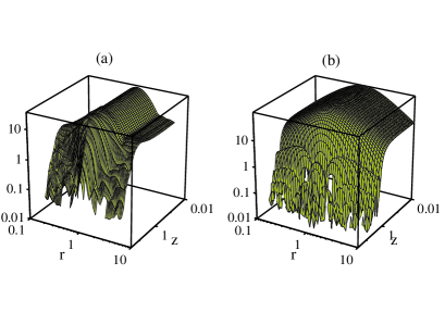
Figure 1: The two point correlation function $C_{11}(z,r)=k^{4}\sqrt{tt^{\prime}}\langle\Phi_{s}({\bf k},t)\Phi_{s}^{*}({\bf k},t^{\prime})\rangle$ is shown. Panel (a) represents the result from numerical simulations of the texture model; panel (b) shows the large-$N$ limit. For fixed $r$ the correlator is constant for $z<1$ and then decays. Note also the symmetry under $r\rightarrow 1/r$.

Figure 2: The correlators $C_{ij}(z,1)$ are shown. The solid, dashed and dotted lines represent $C_{22}~{},~{}C_{11}$ and $|C_{12}|$ respectively. Panel (a) is obtained from numerical simulations of the texture model and panel (b) shows the large-$N$ limit. A striking difference is that the large-$N$ value for $|C_{12}|$ is relatively well approximated by the perfectly coherent result $\sqrt{|C_{11}C_{22}|}$ while the texture curve for $|C_{12}|$ lies nearly a factor 10 lower.

Figure 3: The correlators $C_{ij}(0,r)$ are shown in the same line styles as in Fig. 2, but for $z=0$ as function of $r=t^{\prime}/t$. The stronger decoherence of the texture model is even more evident here.

The UTCs are obtained numerically as functions of the variables $k$, $t$ and $t_{c}$ with $t\geq t_{c}$ and $t_{c}$ fixed. They are then linearly interpolated to the required range. We construct a hermitian $100\times 100$ matrix in $kt$ and $kt^{\prime}$, with the values of $kt$ chosen on a linear scale to maximize the information content, $0\leq kt\leq x_{\mathrm{m}ax}$. The choice of a linear scale ensures good convergence of the sum of the eigenvectors after diagonalization (see  lam ), but still retains enough data points in the critical region, ${\cal O}(x)=1$, where the correlators start to decay. In practice we choose as the endpoint $x_{\mathrm{m}ax}$ of the range sampled by the simulation the value at which the correlator decays by about two orders of magnitude, typically $x_{\mathrm{m}ax}\approx 40$. The eigenvectors that are fed into a Boltzmann code are then interpolated using cubic splines with the condition $v_{n}(kt)\rightarrow 0$ for $kt\gg x_{\mathrm{m}ax}$.

We use several methods to test the accuracy of the simulation: energy momentum conservation of the defects code is found to be better than 10% on all scales larger than about 4 grid units, as is seen in Fig. 4. A comparison with the exact spherically symmetric solution in non-expanding space PST2 shows very good agreement.

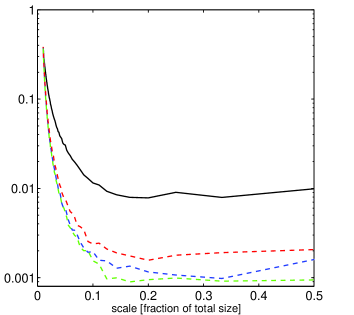
Figure 4: Energy momentum conservation of our numerical simulations is shown. The lines represent the sum of the terms which has to vanish if energy (solid) respectively momentum (dashed) is conserved, divided by the sum of the absolute value of these terms. The abscissa indicates the wavelength of the perturbation as fraction of the size of the entire grid.

The resulting CMB spectrum on Sachs Wolfe scales is consistent with the line of sight integration of Ref. ZD . Furthermore, the overall shape and amplitude of the unequal time correlators are quite similar to those found in the analytic large-$N$ approximation TS ; KD ; DK (see Figs. 1,2 and 3). The main difference of the large-$N$ approximation is that there the field evolution, Eq. (1), is approximated by a linear equation. The non-linearities in the large-$N$ seeds which are due solely to the energy momentum tensor being quadratic in the fields, are much weaker than in the texture model where the field evolution itself is non-linear. Therefore, decoherence which is a purely non-linear effect, is expected to be much weaker in the large-$N$ limit. This is actually the main difference between the two models as can be seen in Fig. 5.

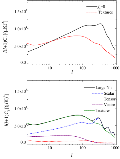
Figure 5: Top panel: the ${\it f_{\pi}}=0$ model. Bottom panel: The $C_{\ell}$ power spectrum is shown for the large-$N$ limit (bold line) and for the texture model. The main difference is clearly that the large-$N$ curve shows some acoustic oscillations which are nearly entirely washed out in the texture case.

III Results and comparison with data

III.1 CMB anisotropies

The $C_{\ell}$’s for the ’standard’ global texture model are shown in Fig. 6 (bottom panel), where a comparison of the full result with the totally coherent approximation (see lam ) is presented.

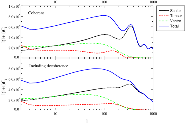
Figure 6: The $C_{\ell}$ power spectrum for the texture scenario is shown in the perfectly coherent approximation (top panel) and in the full eigenfunction expansion. Even in the coherent approximation, the acoustic peaks are not higher than the Sachs Wolfe plateau. Decoherence (see lam ) just washes out the structure but does not significantly damp the peaks.

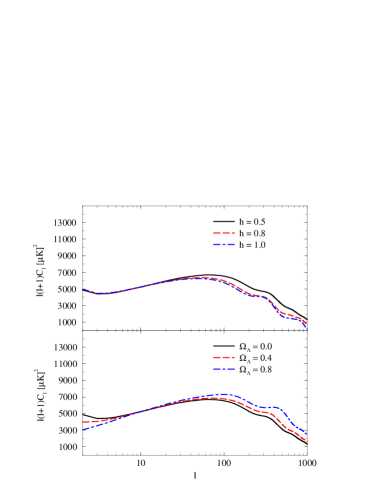
Figure 7: The $C_{\ell}$ power spectrum is shown for different values of cosmological parameters. In the top panel we choose $\Omega_{\Lambda}=0$, $\Omega_{CDM}=0.95$, $\Omega_{b}=0.05$ and vary $h$. In the bottom panel we fix $h=0.5$, $\Omega_{b}=0.05$ and vary $\Omega_{\Lambda}$. We only consider spatially flat universes, $\Omega_{0}=1$.

$\Omega_{\Lambda}$	$h$	$\epsilon$	$\sigma_{8}$
0.0	0.5	$(1.66\pm 0.17)10^{-5}$	0.24
0.0	0.8	$(1.67\pm 0.17)10^{-5}$	0.34
0.0	1.0	$(1.68\pm 0.17)10^{-5}$	0.44
0.4	0.5	$(1.64\pm 0.16)10^{-5}$	0.22
0.8	0.5	$(1.59\pm 0.16)10^{-5}$	0.16

Table 1: The value of the normalization constant $\epsilon$ and the fluctuation amplitude $\sigma_{8}$ are given for the different models considered. The error in $\epsilon$ comes from a best fit normalization to the full CMB data set. Cosmological parameters which are not indicated are identical in all models or given by $\Omega_{0}=\Omega_{cdm}+\Omega_{\Lambda}+\Omega_{b}=1$. We consider only spatially flat models with $\Omega_{b}=0.05$ and a helium fraction of 23%. The parameter choice indicated in the top line is referred to as standard texture model in the text.

Vector and tensor modes are found to be of the same order as the scalar component at COBE-scales. For the ’standard’ texture model we obtain $C_{10}^{(S)}:C_{10}^{(V)}:C_{10}^{(T)}\sim 0.9:1.0:0.3$, in good agreement with the predictions of Refs. PST ; Aetal ; ABR and DK . Due to tensor and vector contributions, even assuming perfect coherence (see Fig. 6, top panel), the total power spectrum does not increase from large to small scales. Decoherence leads to smoothing of oscillations in the power spectrum at small scales and the final power spectrum has a smooth shape with a broad, low isocurvature ’hump’ at $\ell\sim 100$ and a small residual of the first acoustic peak at $\ell\sim 350$. There is no structure of peaks at small scales. The power spectrum is well fitted by the following fourth-order polynomial in $x=\log\ell$:

$${\ell(\ell+1)C_{\ell}\over 110C_{10}}=1.5-2.6x+3.3x^{2}-1.4x^{3}+0.17x^{4}~{}.$$ (6)

The effect of decoherence is less important for the large-$N$ model, where oscillations and peaks are still visible (see Fig 5, bottom panel). This is due to the fact that the non-linearity of the large-$N$ limit is only in the quadratic energy momentum tensor. The scalar field evolution is linear in this limitTS , in contrast to the $N=4$ texture model. Since decoherence is inherently due to non-linearities, we expect it to be stronger for lower values of $N$. COBE normalization leads to $\epsilon=(0.92\pm 0.1)10^{-5}$ for the large-$N$ limit.

In Fig. 7 we plot the global texture $C_{\ell}$ power spectrum for different choices of cosmological parameters. The variation of parameters leads to similar effects like in the inflationary case, but with smaller amplitude. At small scales ($\ell\geq 200$), the $C_{\ell}$s decrease with increasing $H_{0}$ and they increase when a cosmological constant $\Omega_{\Lambda}=1-\Omega_{m}$ is introduced. Nonetheless, the amplitude of the anisotropy power spectrum at high $\ell$s remains in all cases on the same level like the one at low $\ell$s, without showing the peak found in inflationary models. The absence of acoustic peaks is a stable prediction of global $O(N)$ models. The models are normalized to the full CMB data set, which leads to slightly larger values of the normalization parameter $\epsilon=4\pi G\eta^{2}$ than pure COBE normalization. In Table 1 we give the cosmological parameters and the value of $\epsilon$ for the models shown in Fig. 7.

In order to compare our results with current experimental data, we have selected a set of $31$ different anisotropy detections obtained by different experiments, or by the same experiment with different window functions and/or at different frequencies. Theoretical predictions and data of CMB anisotropies are usually compared by plotting the theoretical $C_{\ell}$ curve along with the CMB measurements converted to band power estimates. We do this in the top panel of Fig. 8. The data points raise from large to smaller scales, in contrast to the theoretical predictions of the model. This fashion of presenting the data is surely correct, but lacks informations about the uncertainties in the theoretical model. Therefore we also compare the detected mean square anisotropy, $\Delta^{(Exp)}$ and the experimental 1-$\sigma$ error, $\Sigma^{(Exp)2}$, directly with the corresponding theoretical mean square anisotropy, given by

$$\Delta^{(Th)}={1\over{4\pi}}\sum_{\ell}(2\ell+1)C_{\ell}W_{\ell}~{},$$ (7)

where the window function $W_{\ell}$ contains all experimental details (chop, modulation, beam, etc.) of the experiment.

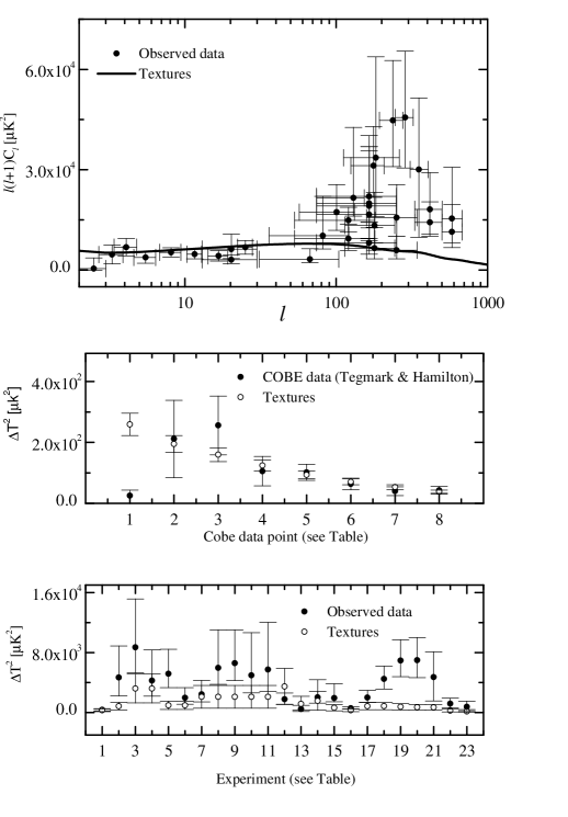
Figure 8: The $C_{\ell}$ spectrum obtained in the standard texture model is compared with data. In the top panel experimental results and the theoretical curve are shown as functions of $\ell$. In the two lower panels we indicate the value of each of the 31 experimental data points with 1-$\sigma$ error bars and the corresponding theoretical value with its uncertainty. The experiments corresponding to a given number are given in Table 2. In the middle panel the 8 COBE data points are shown. In the bottom panel other experiments are presented.

The theoretical error in principle depends on the statistics of the perturbations. If the distribution is Gaussian, one can associate a sample/cosmic variance

$$\Sigma^{(Th)2}={1\over f}{1\over 8\pi^{2}}\sum_{\ell}(2\ell+1)W^{2}_{\ell}C^{2}_{\ell}~{},$$ (8)

where $f$ represents the fraction of the sky sampled by a given experiment.

Deviation from Gaussianity leads to an enhancement of this variance, which can be as large as a factor of $7$ (see xiao ). Even if the perturbations are close to Gaussian (which has been found by simulations on large scales ZD ; ACSSV ), the $C_{\ell}$’s, which are the squares of Gaussian variables, are non-Gaussian. This effect is, however only relevant for relatively low $\ell$s. Keeping this caveat in mind, and missing a more precise alternative, we nevertheless indicate the minimal, Gaussian error calculated according to (8). We add a $30\%$ error from the CMB normalization. The numerical seeds are assumed to be about 10% accurate.

In Table 2, the detected mean square anisotropy, $\Delta^{(Exp)}$, with the experimental 1-$\sigma$ error are listed for each experiment of our data set. The corresponding sky coverage is also indicated. In Fig. 8 we plot these data points, together with the theoretical predictions for a texture model with $h=0.5$ and $\Omega_{\Lambda}=0$.

Experiment	Data point	$\Delta T^{2}(\mu K)^{2}$	$+(\mu K)^{2}$	$-(\mu K)^{2}$	Sky Coverage	Reference	$\chi^{2}_{j}$
COBE1	1	25.2	183	25.2	0.65	tegma	125.29
COBE2	2	212	126	128	0.65	tegma	0.02
COBE3	3	256	96.5	96.9	0.65	tegma	0.49
COBE4	4	105.5	48.3	48.2	0.65	tegma	0.74
COBE5	5	101.9	26.5	26.4	0.65	tegma	0.1
COBE6	6	63.4	19.11	18.9	0.65	tegma	1.11
COBE7	7	39.6	14.5	14.5	0.65	tegma	2.55
COBE8	8	42.5	12.7	12.8	0.65	tegma	0.04
ARGO Hercules	1	360	170	140	0.0024	deb	0.001
MSAM93	2	4680	4200	2450	0.0007	che	0.74
MSAM94	3	4261	4091	2087	0.0007	che2	0.51
MSAM94	4	1960	1352	858	0.0007	che2	0.01
MSAM95	5	8698	6457	3406	0.0007	che3	1.47
MSAM95	6	5177	3264	1864	0.0007	che3	0.30
MAX HR	7	2430	1850	1020	0.0002	tan	0.001
MAX PH	8	5960	5080	2190	0.0002	tan	0.41
MAX GUM	9	6580	4450	2320	0.0002	tan	0.73
MAX ID	10	4960	5690	2330	0.0002	tan	0.17
MAX SH	11	5740	6280	2900	0.0002	tan	0.25
Tenerife	12	3975	2855	1807	0.0124	gut	0.64
South Pole Q	13	480	470	160	0.005	gun	0.52
South Pole K	14	2040	2330	790	0.005	gun	0.01
Python	15	1940	189	490	0.0006	dra	0.37
ARGO Aries	16	580	150	130	0.0024	mas	0.78
Saskatoon	17	1990	950	630	0.0037	net	0.79
Saskatoon	18	4490	1690	1360	0.0037	net	3.83
Saskatoon	19	6930	2770	2140	0.0037	net	4.60
Saskatoon	20	6980	3030	2310	0.0037	net	4.01
Saskatoon	21	4730	3380	3190	0.0037	net	1.32
CAT1	22	934	403	232	0.0001	bak	1.36
CAT2	23	577	416	238	0.0001	bak	0.62

Table 2: The CMB anisotropy detections used in our analysis. The 3., 4. and 5. column denote the value of the anisotropy and the upper and lower 1-$\sigma$ errors respectively. The references are: Tegmark and Hamilton 1997 tegma ; de Bernardis et al. 1994 deb ; Cheng et al. 1994 che ; Cheng et al. 1996 che2 ; Cheng et al. 1997 che3 ; Tanaka et al. 1996 tan ; Gutierrez et al. 1997 gut ; Gundersen et al. 1993 gun ; Dragovan et al. 1993 dra ; Masi et al 1996 mas ; Netterfield et al. 1996 net ; Scott et al. 1997 bak .

We find that, apart from the COBE quadrupole, only the Saskatoon experiment disagrees significantly, more than $1\sigma$, with our model. But also this disagreement is below $3\sigma$ and thus not sufficient to rule out the model. In the last column of Table 2 we indicate

$$\chi_{j}^{2}=(\Delta_{j}^{(Th)}-\Delta_{j}^{(Exp)})^{2}/(\Sigma_{j}^{(Th)2}+\Sigma_{j}^{(Exp)2})$$

for the $j$-th experiment, where the theoretical model is the standard texture model with $\Omega_{\Lambda}=0$ and $h=0.5$. The major discrepancy between data and theory comes from the COBE quadrupole. Leaving away the quadrupole, which can be contaminated and leads to a similar $\chi^{2}$ also for inflationary models, the data agrees quite well with the model, with the exception of three Saskatoon data points. Making a rough chi-square analysis, we obtain (excluding the quadrupole) a value $\chi^{2}=\sum_{j}\chi_{j}^{2}\sim 30$ for a total of 30 data points and one constraint. An absolutely reasonable value, but one should take into account that the experimental data points which we are considering are not fully independent. The regions of sky sampled by the Saskatoon and MSAM or COBE and Tenerife, for instance, overlap. Nonetheless, even reducing the degrees of freedom of our analysis to $N=25$, our $\chi^{2}$ is still in the range $(N-1)\pm{\sqrt{2}(N-1)}\sim 24\pm 7$ and hence still compatible with the data.

This shows that even assuming Gaussian statistics, the models are not convincingly ruled out from present CMB data. There is however one caveat in this analysis: A chi-square test is not sensitive to the sign of the discrepancy between theory and experiment. For our models the theoretical curve is systematically lower than the experiments. For example, whenever the discrepancy between theory and data is larger than $0.5\sigma$, which happens with nearly half of the data points (13), in all cases except for the COBE quadrupole, the theoretical value is smaller than the data. If smaller and larger are equally likely, the probability to have $12$ or more equal signs is $2(13+1)/2^{13}\simeq 3.4\times 10^{-3}$. This indicates that either the model is too low or that the data points are systematically too high. The number $0.003$ can however not be taken seriously, because we can easily change it by increasing our normalization on a moderate cost of $\chi^{2}$.

III.2 Matter distribution

In Table 1 we show the expected variance of the total mass fluctuation $\sigma_{R}$ in a ball of radius $R=8h^{-1}$Mpc, for different choices of cosmological parameters. We find $\sigma_{8}=(0.44\pm 0.07)h$ (the error coming from the CMB normalization) for a flat model without cosmological constant, in agreement with the results of Ref. PST . From the observed cluster abundance, one infers $\sigma_{8}=(0.50\pm 0.04)\Omega^{-0.5}$ eke and $\sigma_{8}=0.59^{+0.21}_{-0.16}$ lid . These results, which are obtained with the Press-Schechter formula, assume Gaussian statistics. We thus have to take them with a grain of salt, since we do not know how non-Gaussian fluctuations on cluster scales are in the texture model. According to Ref. free , the Hubble constant lies in the interval $h\simeq 0.73\pm 0.06\pm 0.08$. Hence, in a flat CDM cosmology, taking into account the uncertainty of the Hubble constant, the texture scenario predicts a reasonably consistent value of $\sigma_{8}$.

As already noticed in Refs. ABR and PST , unbiased global texture models are unable to reproduce the power of galaxy clustering at very large scales, $\stackrel{{\scriptstyle>}}{{\sim}}20h^{-1}$ Mpc. In order to quantify this discrepancy we compare our prediction of the linear matter power spectrum with the results from a number of infrared (fish ,tadr ) and optically-selected (daco , lin ) galaxy redshift surveys, and with the real-space power spectrum inferred from the APM photometric sample (baugh ) (see Fig. 10). Here, cosmological parameters have important effects on the shape and amplitude of the matter power spectrum. Increasing the Hubble constant shifts the peak of the power spectrum to smaller scales (in units of $h/$Mpc), while the inclusion of a cosmological constant enhances large scale power.

We consider a set of models in $\Omega_{\Lambda}$ – $h$ space, with linear bias kais as additional parameter. In Table 3 we report for each survey and for each model the best value of the bias parameter obtained by $\chi^{2}$-minimization. We also indicate the value of $\chi^{2}$ (not divided by the number of data points). The data points and the theoretical predictions are plotted in Fig. 21. Our bias parameter strongly depends on the data considered. This is not surprising, since also the catalogs are biased relative to each other.

Models without cosmological constant and with $h\sim 0.8$ only require a relatively modest bias $b\sim 1.3-3$. But for these models the shape of the power spectrum is wrong as can be seen from the value of $\chi^{2}$ which is much too large. The bias factor is in agreement with our prediction for $\sigma_{8}$. For example, our best fit for the IRAS data, for $h\sim 0.8$ is $b\sim 1.3$. With $\sigma_{8}^{IRAS}=(0.69\pm 0.05)$, this gives $\sigma_{8}\sim 0.48\pm 0.04$, compatible with the direct computation

Whether IRAS galaxies are biased is still under debate. Published values for the $\beta$ parameter, defined as $\beta=\Omega^{0.6}/b$, for IRAS galaxies, range between $\beta_{I}=0.9^{+0.2}_{-0.15}$ kais2 and $\beta_{I}=0.5\pm 0.1$ will . Biasing of IRAS galaxies is also suggested by measurements of bias in the optical band. For example, Ref. pea97 finds $\beta_{o}=0.40\pm 0.12$, in marginal agreement with shai , which obtains $\beta_{o}=0.35\pm 0.1$. A bias for IRAS galaxies is not only possible but even preferred in flat global texture models.

But also with bias, our models are in significant contradiction with the shape of the power spectrum at large scales. As the values of $\chi^{2}$ in Table 3 and Fig. 10 clearly indicate, the models are inconsistent with the shape of the IRAS power spectrum, and they can be rejected with a high confidence level. The APM data which has the smallest error bars is the most stringent evidence against texture models. Nonetheless, these data points are not measured in redshift space but they come from a de-projection of a $2-D$ catalog into $3-D$ space. This might introduce systematic errors and thus the errors of APM may be underestimated.

Catalog	$h$	$\Omega_{\Lambda}$	Best fit bias $b$	$\chi^{2}$	Data points
CfA2-SSRS2 101 Mpc	0.5	0.0	3.4	29	24
CfA2-SSRS2 101 Mpc	0.8	0.0	2.0	40	24
CfA2-SSRS2 101 Mpc	1.0	0.0	1.9	44	24
CfA2-SSRS2 101 Mpc	0.5	0.4	3.9	17	24
CfA2-SSRS2 101 Mpc	0.5	0.8	9.5	4	24
CfA2-SSRS2 130 Mpc	0.5	0.0	5.3	8	19
CfA2-SSRS2 130 Mpc	0.8	0.0	3.4	15	19
CfA2-SSRS2 130 Mpc	1.0	0.0	3.4	16	19
CfA2-SSRS2 130 Mpc	0.5	0.4	5.6	5	19
CfA2-SSRS2 130 Mpc	0.5	0.8	11.1	4	19
LCRS	0.5	0.0	3.0	71	19
LCRS	0.8	0.0	1.8	96	19
LCRS	1.0	0.0	1.6	108	19
LCRS	0.5	0.4	3.7	33	19
LCRS	0.5	0.8	8.7	40	19
IRAS	0.5	0.0	2.3	102	11
IRAS	0.8	0.0	1.3	131	11
IRAS	1.0	0.0	1.3	140	11
IRAS	0.5	0.4	2.8	70	11
IRAS	0.5	0.8	6.3	9	11
IRAS 1.2 Jy	0.5	0.0	4.2	56	29
IRAS 1.2 Jy	0.8	0.0	2.9	92	29
IRAS 1.2 Jy	1.0	0.0	2.9	99	29
IRAS 1.2 Jy	0.5	0.4	4.3	39	29
IRAS 1.2 Jy	0.5	0.8	6.7	28	29
APM	0.5	0.0	3.3	1350	29
APM	0.8	0.0	1.8	1500	29
APM	1.0	0.0	1.7	1466	29
APM	0.5	0.4	3.5	1461	29
APM	0.5	0.8	6.2	1500	29
QDOT	0.5	0.0	4.3	32	19
QDOT	0.8	0.0	2.9	44	19
QDOT	1.0	0.0	2.9	46	19
QDOT	0.5	0.4	4.3	25	19
QDOT	0.5	0.8	7.3	14	19

Table 3: Analysis of the matter power spectrum. In the first column the catalog is indicated. Cols. 2 and 3 specify the model parameters. In cols. 4 and 5 we give the bias parameter inferred by $\chi^{2}$ minimization as well as the value of $\chi^{2}$. Col. 6 shows the number of ’independent’ data points assumed in the analysis.

Models with a cosmological constant agree much better with the shape of the observed power spectra, the value of $\chi^{2}$ being low for all except the APM data. But the values of the bias factors are extremely high for these models. For example, IRAS galaxies should have a bias $b\sim 3-6$, resulting in $\sigma_{8}\leq 0.25$, and in a $\beta_{I}\leq 0.2$ which is too small, even allowing for big variances due to non-Gaussian statistics.

The power spectra for the large-$N$ limit and for the coherent approximation are typically a factor 2 to 3 higher (see Fig. 10), and the biasing problem is alleviated for these cases. For $\Omega_{\Lambda}=0$ we find $\sigma_{8}=0.57h$ for the large-$N$ limit and $\sigma_{8}=0.94h$ for the coherent approximation. This is no surprise since only one source function, $\Psi_{s}$, the analog of the Newtonian potential, seeds dark matter fluctuations and thus the coherence always enhances the unequal time correlator. The dark matter Greens function is not oscillating, so this enhancement translates directly into the power spectrum.

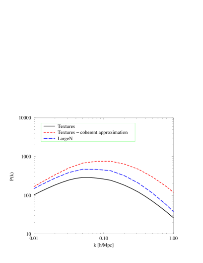
Figure 9: The dark matter power spectrum for the texture model (solid line) is compared with the coherent approximation (short dashed) and the large-$N$ limit (long dashed). The spectra are COBE normalized and the cosmological parameters are $\Omega_{\Lambda}=0~{},~{}h=0.5$.

Models which are anti-coherent in the sense defined in Section IID reduce power on Sachs-Wolfe scales and enhance the power in the dark matter. Anti-coherent scaling seeds are thus the most promising candidates which may cure some of the problems of global $O(N)$ models.

The simple analysis carried out here does not take into account the effects of non-linearities and redshift distortions. Redshift distortions in the texture case should be less important than in the inflationary case since the peculiar velocities are rather low (see next paragraph). Non-linearities typically set in at $k\geq 0.5h$Mpc^-1 and should not have a big effect on our main conclusions which come from much larger scales. Inclusion of these corrections will result in more small-scale power and in a broadening of the spectra, which even enhances the conflict between models and data. Furthermore, variations of other cosmological parameters, like the addition of massive neutrinos, hot dark matter, which is not considered here, will result in a change of the spectrum on small scales but will not resolve the discrepancy at large scales.

Nonetheless, scale dependent biasing may exist and lead to a non-trivial relation between the calculated dark matter power spectrum and the observed galaxy power spectrum. We are thus very reluctant to rule out the model by comparing two in principle different things, the relation of which is far from understood. Therefore we would prefer to reject the models on the basis of peculiar velocity data, which is more difficult to measure but most certainly not biased.

Figure 10: Matter Power spectrum: comparison between data and theory. References are in the text. Data set courtesy of M. S. Vogeley voegel .

III.3 Bulk velocities

To get a better handle on the missing power on 20 to 100$h^{-1}$Mpc, we investigate the velocity power spectrum which is not plagued by biasing problems. The assumption that galaxies are fair tracers of the velocity field seems to us much better justified, than to assume that they are fair tracers of the mass density. We therefore test our models against peculiar velocity data. We use the data by Ref. deke which gives the bulk flow

$$\sigma^{2}_{v}(R)={H_{0}^{2}\Omega_{m}^{1.2}\over{2\pi^{2}}}\int P(k)W(kR)dk~{},$$ (9)

in spheres of radii $R=10$ to $60h^{-1}$Mpc. These data are derived after reconstructing the $3-$dimensional velocity field with the POTENT method (see deke and references therein).

As we can see from Table 4, the COBE normalized texture model predicts too low velocities on large scales when compared with POTENT results. Recent measurements of the bulk flow lead to somewhat lower estimates like $\sigma_{v}(R)\sim(230\pm 90)$ at $R=60h^{-1}$Mpc (giova ), but still a discrepancy of about a factor of $2$ in the best case remains.

Including a cosmological constant helps at large scales, but decreases the velocities on small scales.

If the observational bulk velocity data is indeed reliable (there are some doubts about thisMark ), all global $O(N)$ models are ruled out.

R	$\sigma_{v}$ (R)	$\Delta_{v}$	$h=0.5$	$h=1.0$	$\Omega_{\Lambda}=0.8$
10	494	170	145	205	86
20	475	160	100	134	78
30	413	150	80	98	70
40	369	150	67	78	65
50	325	140	57	65	61
60	300	140	50	56	57

Table 4: Bulk velocities: Observational data from deke and theoretical predictions. $\Delta_{v}$ estimates the observational uncertainty. The uncertainties on the theoretical predictions are around $\sim 30\%$. The models $\Omega_{\Lambda}=0$ with $h=0.5$ and $h=1$ as well as $\Omega_{\Lambda}=0.8,~{}h=0.5$ are investigated.

IV Conclusions

We have determined CMB anisotropies and other power spectra of linear perturbations in models with global $O(N)$ symmetry which contain global monopoles and texture. Our main results can be summarized as follows:

• Global $O(N)$ models predict a flat spectrum (Harrison-Zeldovich) of CMB anisotropies on large scales which is in good agreement with the COBE results. Models with vanishing cosmological constant and a large value of the Hubble parameter give $\sigma_{8}\sim 0.4$ to $0.5$ which is reasonable.

• Independent of cosmological parameters, these models do not exhibit pronounced acoustic peaks in the CMB power spectrum.

• The dark matter power spectrum from global $O(N)$ models with $\Omega_{\Lambda}=0$ has reasonable amplitude but does not agree in its shape with the galaxy power spectrum, especially on very large scales $>20h^{-1}$Mpc.

• Models with considerable cosmological constant agree relatively well with the shape of the galaxy power spectrum, but need very high bias $b\sim 4-6$ even with respect to IRAS galaxies.

• The large scale bulk velocities are by a factor of about 3 to 5 smaller than the values inferred from deke .

In view of the still considerable errors in the CMB data (see Fig. 8), and the biasing problem for the dark matter power spectrum, we consider the last argument as the most convincing one to rule out global $O(N)$ models. Even if velocity data is quite uncertain, observations agree that bulk velocities on the scale of $50h^{-1}$Mpc are substantially larger than the (50 – 70)km/s obtained in texture models.

However, all our constraints have been obtained assuming Gaussian statistics. We know that global defect models are non-Gaussian, but we have not investigated how severely this influences the above conclusions. Such a study, which we plan for the future, requires detailed maps of fluctuations, the resolution of which is always limited by computational resources. Generically we can just say that non-Gaussianity can only weaken the above constraints.

Our results naturally lead to the question whether all scaling seed models are ruled out by present data. The main problem of the $O(N)$ model is the missing power at intermediate scales, $\ell\sim 300-500$ or $R\sim(20-100)h^{-1}{\rm Mpc}$. We have briefly investigated whether this problem can be mitigated in a scaling seed model without vector and tensor perturbations. In this case, also scalar anisotropic stresses are reduced by causality requirements (see Ref. DK ), and perturbations on superhorizon scaled are compensated (see DS ). For simplicity, we analyze a model with purely scalar perturbations and no anisotropic stresses at all, $f_{\pi}=0$. The seed function $\Phi_{s}$ is taken from the texture model (numerical simulations) and we set $\Psi_{s}=-\Phi_{s}$. The resulting CMB anisotropy spectrum is shown in Fig. 5, top panel. A smeared out acoustic peak with an amplitude of about $2.2$ does indeed appear in this model. This is mainly due to fluctuations on large scales being smaller, as is also evident from the higher value of $\epsilon=(2.2\pm 0.2)\times 10^{-5}$. But also here, the dark matter density fluctuations and bulk velocities are substantially lower than observed galaxy density fluctuations or the POTENT bulk flows.

Clearly, this simple example is not sufficient and a more thorough analysis of generic scaling seed models is presently under investigation. So far it is just clear that contributions from vector and tensor perturbations are severely restricted.
Acknowledgment
It is a pleasure to thank Andrea Bernasconi, Paolo de Bernardis, Roman Juszkiewicz, Mairi Sakellariadou, Paul Shellard, Andy Yates and Marc Davis for stimulating discussions. Our Boltzmann code is a modification of a code worked out by the group headed by Nicola Vittorio. We also thank Michael Vogeley who kindly provided us the galaxy power spectra shown in our figures. The numerical simulations have been performed at the Swiss super computing center CSCS. This work is partially supported by the Swiss National Science Foundation.

References

-
(1)
See the web sites:
http://astro.estec.esa.nl/SA-general
/Projects/Planck/
and http://map.gsfc.nasa.gov/ - (2) W. Hu, N. Sugiyama and J. Silk, Nature 386, 37 (1995).
- (3) R. Durrer and M. Kunz, Phys, Rev. D 57, R3199 (1998).
- (4) U. Pen, U. Seljak and N. Turok, Phys. Rev. Lett. 79, 1611 (1997).
- (5) P.P. Avelino, E.P.S. Shellard, J.H.P. Wu and B. Allen, Phys. Rev. Lett., in print (archived under astro-ph/9712008) (1998).
- (6) R. Durrer and Z. Zhou, Phys. Rev. D 53, 5394 (1996).
- (7) R. Durrer, M. Kunz and A. Melchiorri, dubmitted to Phys. Rev. D (1998); preprint archived under astro-ph/9811174.
- (8) U. Pen, D. Spergel and N. Turok, Phys Rev. D 49, 692 (1994).
- (9) W. P. Petersen and A. Bernasconi, CSCS Technical Report TR-97-06 (1997).
- (10) N. Turok and D. Spergel, Phys. Rev. Lett. 64, 2736 (1990).
- (11) M. Kunz and R. Durrer, Phys. Rev. D 55, R4516 (1997).
- (12) B. Allen et al., Phys. Rev. Lett. 79, 2624 (1997).
- (13) A. Albrecht, R. Battye and J. Robinson, Phys. Rev. Lett. 79, 4736 (1997).
- (14) X. Luo, Astrophys. J. 439, 517L (1995) .
- (15) B. Allen et al., Phys. Rev. Lett 77, 3061 (1996).
- (16) M. Tegmark and A. Hamilton, archived under astro-ph/9702019 (1997)
- (17) P. de Bernardis et al., Astrophys. J. 422, 33L (1994).
- (18) E.S. Cheng et al., Astrophys. J. 422, 40L (1994).
- (19) E.S. Cheng et al., Astrophys. J. 456, 71L (1996).
- (20) E.S. Cheng et al., Astrophys. J.488, 59L (1997).
- (21) A. Albrecht, R. Battye and J. Robinson, Phys. Rev. Lett. 79, 4736 (1997).
- (22) S.T. Tanaka et al., Astrophys. J. 468, 81L (1996).
- (23) C. M. Gutierrez et al., Astrophys. J. 480, 83L (1997).
- (24) J.O. Gundersen et al., Astrophys. J.413, 1L (1993).
- (25) M. Dragovan et al., Astrophys. J.427, 67L (1993).
- (26) S. Masi et al., Astrophys. J.463, 47L (1996).
- (27) B. Netterfield et al., Astrophys. J.474, 47 (1997).
- (28) P.F. Scott at al., Astrophys. J.461, 1L (1996).
- (29) V.R. Eke, S. Cole and C.S. Frenk M.N.R.A.S. 282, 263E (1996).
- (30) A.R. Liddle, D. Lyth, H. Robeerts, P. Viana, M.N.R.A.S. 278, 644 (1996).
- (31) W. Freedman, J.R. Mould, R.C. Kennicut and B.F. Madore, archived under astro-ph/9801080 (1998).
- (32) K.B. Fisher, M. Davis, M.A. Strauss, A. Yahil and J.P. Huchra, M.N.R.A.S. 266, 50 (1994).
- (33) H. Tadros and G. Efstathiou, M.N.R.A.S., L45, 276 (1995).
- (34) L.N. Da Costa, M.S. Vogeley, M.J. Geller, J.P. Huchra and C. Park, Astrophys. J. 437, 1L (1994).
- (35) H. Lin et al., AAS, 185, 5608L (1994).
- (36) C.M. Baugh and G. Efstathiou, M.N.R.A.S., 265, 145 (1993).
- (37) N. Kaiser, Astrophys. J. 284, 9L (1984).
- (38) N. Kaiser, G. Efstathiou, R. Ellis, C.S. Frenk, A. Lawrence, M. Rowan-Robinson and W. Saunders, M.N.R.A.S. 252, 1 (1991).
- (39) J.A. Willick, S. Courteau, S.M. Faber, D. Burstein, A. Dekel and T. Kolatt, Astrophys. J. 457, 460 (1996).
- (40) J.A. Peacock, M.N.R.A.S. 284, 885P (1997).
- (41) E.J. Shaia, P.J.E. Peebles and R.B. Tully, Astrophys. J. 454, 15 (1995).
- (42) A. Dekel, Ann. Rev. of Astron. and Astrophys. 32, 371 (1994).
- (43) R. Giovanelli et al., preprint, archived under astro-ph/98707274 (1998).
- (44) M.S. Vogeley, to appear in ”Ringberg Workshop on Large-Scale Structure”, ed. D. Hamilton, (Kluwer, Amsterdam), archived under astro-ph/9805160 (1998).
- (45) M. Davis, private communication (1998).
- (46) R. Durrer and M. Sakellariadou, Phys. Rev. D 56, 4480 (1997).