Magnetic Lensing near Ultramagnetized Neutron Stars

Abstract

Extremely strong magnetic fields change the vacuum index of refraction. This induces a lensing effect that is not unlike the lensing phenomenon in strong gravitational fields. The main difference between the two is the polarization dependency of the magnetic lensing, a behaviour that induces a handful of interesting effects. The main prediction is that the thermal emission of neutron stars with extremely strong magnetic fields is polarized - up to a few percent for the largest fields known. This potentially allows a direct method for measuring their magnetic fields.

1 Introduction

The most intense magnetic fields in the universe are found near neutron stars. Soon after the discovery of radio pulsars ([Hewish et al. 1968]), [Gold 1968] argued that the steady increase in their periods could be explained if they were strongly magnetized neutron stars with dipolar fields of $\sim 10^{12}$ G. Since that time, the variety of radio pulsars has expanded. These neutron stars have magnetic fields ranging from $10^{8}$ G for the millisecond pulsars to $2.1\times 10^{13}$ G for PSR 0157+6212 ([Arzoumanian et al. 1994]), the most strongly magnetized radio pulsar discovered to date.

A dozen years after the discovery of radio pulsars, the increased scrutiny of the sky at $\gamma$-ray energies uncovered a new class of objects, the soft-gamma repeaters (SGRs). In the most successful model for these energetic sources, the crust of a strongly magnetized ($B\sim 10^{14-15}$ G) neutron star or “magnetar” periodically fractures, releasing a large amount of energy into the magnetosphere which is observed as soft-gamma radiation ([Thompson & Duncan 1995]). Until the past year, the evidence for the intense magnetic fields surrounding SGRs was circumstantial. As [Gold 1968] argued for radio pulsars, [Kouveliotou et al. 1998a] precisely measured the spin down of SGR 1806-20 and inferred a dipole field of $8\times 10^{14}$ G. [Kouveliotou et al. 1998b] measured ${\dot{P}}$ of SGR 1900+14 and find it to be consistent with $B=2-8\times 10^{14}$ G.

In the past decade, more sensitive X-ray telescopes have also discovered a new class of sources which may have extremely strong magnetic fields. The anomalous X-ray pulsars (AXP) are soft X-ray sources and they are often associated with supernova remnants. Unlike the majority of X-ray pulsars, these objects have periods of several seconds which steadily and quickly increases. Furthermore, no binary companions have been found near these objects. Although no single picture has yet emerged to explain AXPs, a strong candidate model is that a neutron star cooling through a strongly magnetized envelope ([Heyl & Hernquist 1997c]) or the decay of a neutron star’s strong magnetic field ([Heyl & Kulkarni 1998]; [Thompson & Duncan 1996]) powers the X-ray emission from these objects. Furthermore, such a strong magnetic field ($B\sim 10^{15}$ G) can also account for the observed spin-down rate of these objects (e.g. [Vasisht & Gotthelf 1997]).

Intense magnetic fields of $B\ga 10^{12}$ G strongly affect physical process in and near neutron stars – ranging from cooling ([Heyl & Hernquist 1997d]; [Shibanov et al. 1995]), to atmospheric emission ([Rajagopal, Romani & Miller 1997]; [Pavlov et al. 1994]) and to the insulation of the core ([Heyl & Hernquist 1998b]; [Heyl & Hernquist 1998a]; [Schaaf 1990a]; [Hernquist 1985]). Yet stronger fields such as those associated with AXPs and SGRs alter the propagation of light through the magnetosphere by way of quantum-electrodynamic (QED) processes and may further process the emergent radiation ([Heyl & Hernquist 1997a]; [Heyl & Hernquist 1997b]; [Baring 1995]; [Baring & Harding 1995]; [Adler 1971]).

Not only will QED alter the spectra from these objects, it also creates a lens surrounding the neutron star which magnifies and reimages the surface. In a sufficiently strong field, the index of refraction for photons with their magnetic fields directed perpendicularly to the local magnetic field can be significantly larger than unity ([Heyl & Hernquist 1997b]). Furthermore, it is a strong function of both the strength of the magnetic field and its direction. In this paper, we will examine the effects of magnetic lensing on the observations of strongly magnetized neutron stars.

2 Index of refraction

In the presence of a strong external field, the vacuum reacts, becoming magnetized and polarized. The index of refraction, magnetic permeability, and dielectric constant of the vacuum are straightforward to calculate using quantum electrodynamic one-loop corrections ([Klein & Nigam 1964a], [Klein & Nigam 1964b], [Erber 1966], [Adler 1971], [Berestetskii, Lifshitz & Pitaevskii 1982], [Mielnieczuk, Lamm & Valluri 1988]). [Heyl & Hernquist 1997b] calculate the index of refraction as a function of field strength to the one loop order. The magnetic field will strongly bend light as it propagates only if $n-1\sim 1$.

For $B\gg\ B_{\hbox{\rm\scriptsize QED}}\approx 4.4\times 10^{13}$ G, the index of refraction becomes significantly larger than unity if the wave has its magnetic field polarized perpendicular to the local magnetic field ($\perp$-mode). To one loop, the waves with their magnetic field directed in the plane containing the local magnetic field, ${\bf B}$, and the wavenumber, ${\bf k}$ ($\parallel$-mode), have $n_{\parallel}-1<\alpha/(6\pi)$ regardless of the strength of the field ($\alpha$, the fine-structure constant is approximately $1/137.04$). This second mode is essentially unaffected by lensing.

In fields where $n_{\perp}-1\sim 1$, [Heyl & Hernquist 1997b] find that $n_{\perp}-1\propto B$ with sufficient precision. Specifically, for $B>B_{\hbox{\rm\scriptsize QED}}/2$

$$n_{\perp}{\hskip-4.0pt}\hskip-4.0pt = \hskip-3.0pt{\hskip-4.0pt}1+\frac{\alpha}{4\pi}\sin^{2}\theta\Biggr{[}\frac{2}{3}\xi-\left(8\ln A-\frac{1}{3}-\frac{2}{3}\gamma\right)$$ (1)

$${\hskip-4.0pt}{\hskip-4.0pt}-\left(\ln\pi+\frac{1}{18}\pi^{2}-2-\ln\xi\right)\xi^{-1}-\left(-\frac{1}{2}-\frac{1}{6}\zeta(3)\right)\xi^{-2}$$

$${\hskip-4.0pt}{\hskip-4.0pt}-\sum_{j=3}^{\infty}\frac{(-1)^{j-1}}{2^{j-2}}\left(\frac{j-2}{j(j-1)}\zeta(j-1)+\frac{1}{6}\zeta(j+1)\right)\xi^{-j}\Biggr{]}$$

$${\hskip-4.0pt}{\hskip-4.0pt}+{\cal O}\left[\left(\frac{\alpha}{2\pi}\right)^{2}\right],$$

where $\xi=B/B_{\hbox{\rm\scriptsize QED}}$ and $\theta$ is the angle between ${\bf B}$ and ${\bf k}$. $\gamma$ is Euler’s constant and $\ln A$ is related to the derivative of the zeta function: $\ln A\equiv 1/12-\zeta^{(1)}(-1)=0.2487...$ . The linear approximation is accurate to 20 % for the value of $n-1$ for fields stronger than $3.9\times 10^{14}$ G where $n-1=2.9\times 10^{-3}$. For this same field strength, $n-1$ for the parallel polarization is ten times smaller. For stronger fields this ratio increases. Thus, we set $n_{\parallel}=1$.

The function $f(B)\equiv(n_{\perp}-1)/\sin^{2}\theta$ contains the portion of the index of refraction which depends on the strength of the external field. The linear approximation is given by $f(B)=\alpha/(6\pi)\times B/B_{\hbox{\rm\scriptsize QED}}\equiv B/B_{0}$. The second loop corrections to the index of refraction are expected to be smaller by a factor of $\alpha$ regardless of the strength of the field ([Dittrich & Reuter 1985]).

3 $\perp$-Ray propagation

In the limit of geometric optics, light rays obey Hamilton’s equations with $H=\omega=ck/n({\bf k},{\bf x})$ ([Landau & Lifshitz 1987], §53). Since the index of refraction depends both on position and wavevector, the resulting equations are nontrivial,

$${\dot{\bf x}}=\nabla_{k}\omega~{}{\hbox{\rm and}}~{}{\dot{\bf k}}=-\nabla_{x}\omega.$$ (2)

Each of these gradients may be calculated for the $\perp$-mode using the index of refraction, $n_{\perp}=1+[1-({\bf k\cdot B}/kB)^{2}]f(B)$:

$$\nabla_{\!x}\omega = {ckf\over n_{\perp}^{2}}\Bigg{[}-\Big{(}{d\ln f\over d\ln B}\sin^{2}\theta+2\cos^{2}\theta\Big{)}{{\bf\nabla}B\over B}$$ (3)

$$\hfill+2\cos\theta{{\bf\nabla}({\bf k\cdot B})\over kB}\Bigg{]}$$

$$\nabla_{\!k}\omega = {c\over n_{\perp}}\frac{{\bf k}}{k}+{2cf\over n_{\perp}^{2}}\cos\theta\Big{(}{{\bf B}\over B}-\cos\theta{{\bf k}\over k}\Big{)}\ .$$ (4)

As outlined in the previous section, the propagation depends on the polarization of the photon; thus, it is important to understand how the photon’s polarization evolves as the direction of the field changes.

3.1 Polarization evolution

As the waves travel through the magnetosphere, they stay in the same polarization mode (parallel or perpendicular) as long as

$$\frac{n_{\|}}{n_{\perp}}\frac{1+n_{\perp}^{2}}{\Delta k}\frac{1}{r_{n}}\ll 1$$ (5)

where $r_{n}$ is the distance over which the magnetic field rotates by one radian and $\Delta k$ is the difference between the wavenumbers of the two polarizations. Evidently, the adiabatic approximation holds for the vicinity of the systems of interest (see [Heyl & Shaviv 1998] for further details).

A photon’s polarization will decouple from the magnetically induced polarization modes at a distance from the star which depends on the strength of the field at the stellar surface and the energy of the photon. Higher frequency photons decouple later; therefore, the observed polarization direction will depend on photon energy with higher frequency photons tracing the magnetic moment of the star projected onto the sky from later in the star’s rotation.

Generally, the wavelength of the photons is much shorter than the length over which the field geometry changes, so the decoupling occurs where the magnetic field is much less than the QED critical value. In this limit, the wave decouples from the field after traveling for a time,

$$t_{\hbox{\rm\scriptsize decouple}}\approx 4.6\hskip 2.0pt{\hbox{\rm ms}}\hskip 2.0pt{\hskip-4.0pt}\left(\frac{E}{1~{}{\hbox{\rm keV}}}\right)^{1/5}{\hskip-4.0pt}\left(\frac{B_{p}\sin\theta}{10^{14}~{}{\hbox{\rm G}}}\right)^{2/5}{\hskip-4.0pt}\left(\frac{R}{10~{}{\hbox{\rm km}}}\right)^{6/5}{\hskip-4.0pt},$$ (6)

where $B_{p}$ is the strength of the magnetic field at the surface, $R$ is the radius of the neutron star and $E$ is the energy of the photon.

The typical value of $t_{\hbox{\rm\scriptsize decouple}}$ for high $B$ neutron stars is such that decoupling will take place well within the light cylinder yet far enough from the stellar surface such that the local magnetic field where the photons decouple is aligned with the apparent magnetic axis, irrespective from where the photons originated. This simplifies the calculation of the two polarization images – The two principle polarization directions at the observer are the $\parallel$ and $\perp$ modes even though the polarization directions from where the photons orginiated were different.

4 The appearance of a magnetar

The nontrivial index of refraction depends on the direction and magnitude of the local magnetic field. Light rays will therefore travel in bent trajectories and the optical appearance of the magnetized neutron star will therefore not be trivial. From equivalent optical configurations (e.g. a black body embedded within a nonspherical medium of index $n$), it is clear that the images of the star will be distorted and can have a varying apparent surface area, even though it is spherical.

We use the ray tracing algorithm to find the image of a magnetar having a dipole magnetic field. For each observing direction characterized by an inclination angle above the magnetic equator, a different image may result. These images can be compared to the unmagnetized case which adequately describes the $\parallel$ polarization. Each image can then be averaged in order to compose a light curve. And finally, all the images can be properly averaged together, to get the total emission properties of the NS.

4.1 The ray tracing algorithm

Using the Hamiltonian formalism and the related adiabatic and geometrical optics approximations (which hold extremely well in our limit), we know that each polarization mode (either the $\parallel$ or $\perp$ modes) will evolve separately according to eq. 2:

$$\dot{\bf x}_{\perp,\parallel}=\nabla_{k}\omega_{\perp,\parallel}~{}~{}{\hbox{\rm and}}~{}~{}\dot{\bf k}_{\perp,\parallel}=-\nabla_{x}\omega_{\perp,\parallel}.$$ (7)

Since we are interested in the regime in which the index of refraction $n_{\parallel}$ of the $\parallel$-mode can be assumed to be 1, its evolution becomes trivial. The image observed in the $\perp$ polarization will not however be straight forward and its light ray trajectories will be bent.

To construct the image observed by a distant observer, we can use the time reversal symmetry of the light trajectory and trace the light rays from the observer to the NS and not vice versa. We place a screen at a large distance from the star and divide it into pixels at the desired resolution (e.g. $300^{2}$). From each pixel, we trace back the path of a light ray leaving in a direction perpendicular to the screen. The ray is then followed until it intersects the NS surface or until it is found to have an increasing radial component, implying that it has missed the star. The configuration is depicted in figure 1.

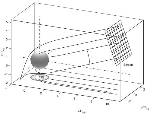
Figure 1: The ray tracing algorithm. Ray trajectories are followed from a distant screen towards the star using the Hamiltonian equations of motion. The rays can then either intersect the star or miss it. Since the magnetic field is assumed to be that of a dipole (aligned with the $z$-axis), it has axial symmetry and different images will be distinguishable by the observer’s magnetic inclination angle $i$.

It is clear from Kirchhoff’s law that if we look at a light ray trajectory that intersects the surface, then if the observer and the object are in thermal equilibrium, we will find that the specific intensity $I$ (flux per unit sterad) of the ray going from the observer to the object should be equal to that of the opposite ray going from the star. Since the observer is at a large distance and has $n\rightarrow 1$ in its vicinity, the specific intensity is just $I=B(T)=\sigma T^{4}/\pi$, where $B(T)$ is the black-body source function (once the ray is in an $n=1$ region). Hence, if the emission from the NS is that of a black-body, then the rays coming from each element will simply carry a specific intensity of $B(T)$ where $T$ is the local effective photospheric temperature at the point where the ray intersects the surface. If the NS has a uniform temperature then the flux observed by an observer at a given direction is simply proportional to the solid angle subtended by the object. As we shall see, this apparent solid angle will be larger from all $4\pi$ possible observer directions implying that the total luminosity emitted at a given temperature is larger in the presence of a magnetic field. This does not necessarily imply that a magnetized NS will shine brighter. As we shall see in §5, the changed surface properties will reduce the temperature to compensate for the higher emission efficiency, leaving an unchanged luminosity.

4.2 Image properties

A few resulting images can be seen in figure 2 which depicts the magnetic latitude and longitude observed at several inclinations for both a weak field and a strong one. We find that in the limit of a weak field (one for which the correction to the index of refraction is less than half), the effects of the magnetic lensing are to slightly distort the image through the imaging of otherwise inaccessible surfaces (surfaces that do not have a direct line of sight) and to have the images appear to subtend a larger surface area. In strong fields with corrections larger than a half to the index of refraction, on the other hand, the images are distorted enough as to have a topologically nontrivial image form in which some surfaces are seen twice (or more) with changing parities.

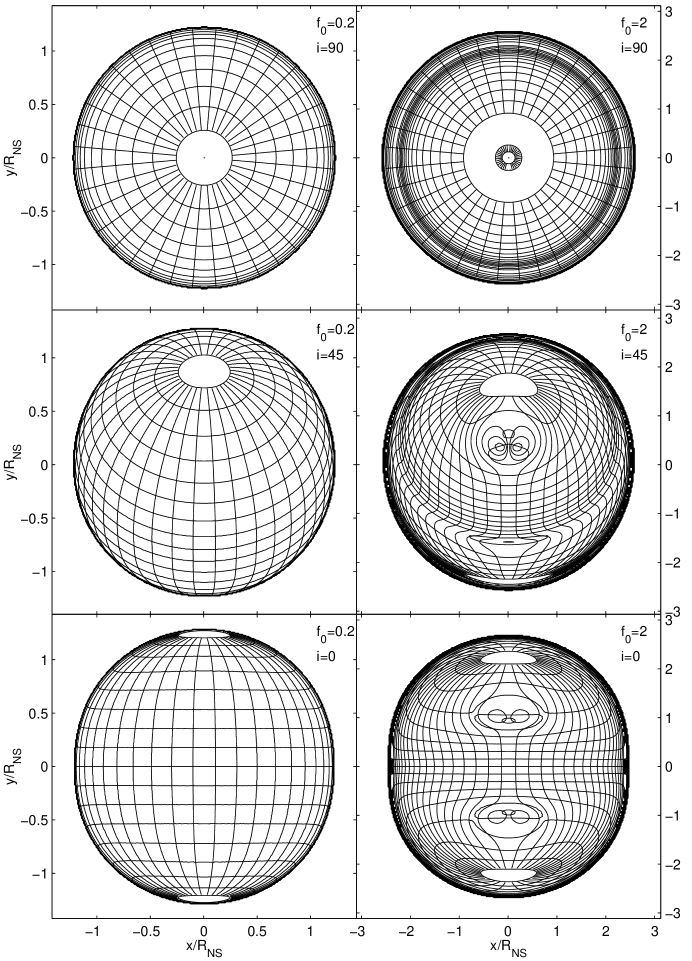
Figure 2: The magnetic latitude and longitude of the surface of the NS as seen with the $\perp$ polarization by a distant observer at different inclinations above the magnetic equator (with spacing of $10^{\circ}$ in each direction). The equatorial magnetic field strengths of $2.3\times 10^{16}$ G and $2.3\times 10^{17}$ G corresponding to $f_{0}=0.2$ and $f_{0}=2.0$. An observer of a “weak” field NS will see a larger image and more than $2\pi$ sterad of the surface. If the NS is a black-body, more light will be seen with the $\perp$ polarization than with the $\parallel$ polarization (for which the image is unchanged). An observer of a highly magnetized NS will see a more complex image in which the same surface element can appear twice (or even more).

The critical equatorial field needed to trigger the nontrivial behaviour is $2.8\times 10^{16}$ G for which $f_{0}\equiv f(B_{\hbox{\rm\scriptsize equator}})=0.25$ on the equator and $f(B_{\hbox{\rm\scriptsize pole}})=0.5$ on the poles. At the latter field strength (for which $n_{\perp}$ can reach $1.5$), the group velocity is no longer a monotonic function of ${\bf k}$, allowing multiple light ray solutions with the same ${\bf v}_{\hbox{\rm\scriptsize g}}$ (3 instead of 1).

If the NS has a uniform surface temperature, its luminosity will just be proportional to the surface area observed. This apparent surface area as a function of the magnetic inclination $i$ of the observer can be well fitted with the following functional form:

$$A^{\prime}=a_{0}+\sum_{n=1}^{4}a_{n}\cos^{n}(2i).$$ (8)

One can also define an asymmetry parameter as the normalized difference between the area observed above the equator and that observed above the pole:

$${\cal A}\equiv{A^{\prime}(i=0^{\circ})-A^{\prime}(i=90^{\circ})\over A^{\prime}(i=0^{\circ})+A^{\prime}(i=90^{\circ})}={(a_{1}+a_{3})\over a_{0}}$$ (9)

The value of the fit parameters and the total asymmetry are shown in figure 3. Evidently, one finds simple expressions for the fitting constants in the limit of weak fields:

$${\cal A}{\hskip-4.0pt}{\hskip-4.0pt} \approx {\hskip-4.0pt}{\hskip-4.0pt}0.095f_{0}={B_{0}\over 1.20\times 10^{18}G}~{}~{}{\hbox{\rm for}}~{}~{}B_{0}\la 10^{16}G~{}~{}{\hbox{\rm and:}}$$ (10)

$$a_{1}{\hskip-4.0pt}{\hskip-4.0pt} \approx {\hskip-4.0pt}{\hskip-4.0pt}0.89{\cal A},~{}a_{2}\approx-0.08{\cal A},~{}a_{3}\approx 0.11{\cal A},~{}a_{4}\approx-0.04{\cal A}.$$

With this fit, we can construct a light curve for a thermally uniform rotating NS.

Figure 3: The fit parameters and the polar/equatorial asymmetry describing the image area for an isothermal NS.

4.3 Average properties

When a surface element is emitting black-body radiation into vacuum, we know from Stefan-Boltzmann’s law that the emitted flux is simply $F=\sigma T^{4}$. Therefore, the intensity of each ray is $I=B(T)\equiv\sigma T^{4}/\pi$. This is however changed when the element is emitting the black-body photons into a medium with a different index of refraction. The reason is that in the presence of $n\neq 1$, there are on one hand more photon states for a given energy band and on the other, the group velocity which relates the density of states to the flux is smaller. For a nondispersive medium with an isotropic index of refraction, the two factors are $n^{3}$ and $1/n$ respectively, implying that a unit surface will emit a flux of $F=\sigma T^{4}n^{2}$, as if the surface area is effectively larger. We can therefore define an effective surface area as the equivalent area relevant for the Stefan-Boltzmann law of the emitted flux if the object would have emitted the photons into vacuum. That is:

$$A_{\hbox{\rm\scriptsize max}}\equiv\int{F\over\sigma T^{4}}dA.$$ (11)

where $A_{\hbox{\rm\scriptsize max}}$ is the effective surface area (and the notation will soon be clear).

A careful analysis shows however that there there is a second relevant definition of an effective area. If an objects of surface area $A$ and temperature $T$ emits radiation into vacuum, then the total luminosity observed through a distant surface surrounding the $4\pi$ sterad around the object, will simply be:

$$L=A\sigma T^{4}.$$ (12)

We can therefore define an effective surface area when the index of refraction is not unity as:

$$A_{\hbox{\rm\scriptsize eff}}\equiv{L\over\sigma T^{4}}.$$ (13)

Under normal circumstances, we expect that the total flux emitted by a surface is the total flux observed at infinity. Namely, that $A_{\hbox{\rm\scriptsize eff}}=A_{\hbox{\rm\scriptsize max}}$. However, this need not be the case if some of the light trajectories leaving the surface intersect the surface again, or in other words, if there is photon trapping. Generally, we can expect that:

$$A_{\hbox{\rm\scriptsize eff}}\leq A_{\hbox{\rm\scriptsize max}}(=An^{2}~{}{\hbox{\rm if}}~{}n~{}{\hbox{\rm is isotropic}}).$$ (14)

There are two effective surface areas and both of them are interesting. The messy calculation of $A_{\hbox{\rm\scriptsize max}}$, the maximum theoretical effective surface area, is found in the appendix. Its results are compared with the observed effective surface area $A_{\hbox{\rm\scriptsize eff}}$ calculated here.

The effective area $A_{\hbox{\rm\scriptsize eff}}$ of the star which is the total area as observered from infinity, is related to the apparent area $A^{\prime}$ seen at various inclinations through the following average:

$$A_{\hbox{\rm\scriptsize eff}}=4\int_{i=0}^{\pi/2}A^{\prime}(i)\cos(i)di,$$ (15)

The definitions are such that in the unlensed limit, the image has $A^{\prime}$ of $\pi R^{2}$ while the surface areas $A_{\hbox{\rm\scriptsize max}}$ and $A_{\hbox{\rm\scriptsize eff}}$ are both $4\pi R^{2}$. The effective surface area can be directly related to the expansion of $A^{\prime}$ found in eq. 8 through its integration, giving that $A_{\hbox{\rm\scriptsize eff}}/4=a_{0}+a_{1}/3+7a_{2}/15+9a_{3}/35+107a_{4}/315$. It is however calculated directly in order to obtain high accuracy.

$A_{\hbox{\rm\scriptsize eff}}$ is calculated using the ray tracing algorithm. For a given magnetic field $B_{0}$ and an observer inclination $i$ above the magnetic equator, the apparent surface area $A^{\prime}$ is calculated. Since the surface brightness of the isothermal NS is the same in each direction in which light rays intersect the NS, one can achieve a high accuracy without the division of the screen into many pixels but instead use a more sophisticated algorithm. Instead, the accuracy is achieved through the accurate measurement of the apparent ‘edge’ of the NS at different angles relative to the center of the screen (through consecutive bisections) and then an integration over angle gives an accurate area measurement - $A^{\prime}(i)$. This area can in turn be integrated to give $A_{\hbox{\rm\scriptsize eff}}$.

The result for different magnetic field strengths can be seen in figure 4 which includes also the total emitted radiation from the surface $A_{\hbox{\rm\scriptsize max}}$ as calculated in the appendix.

Figure 4: The effective area of the NS when observed with the $\perp$ polarization. For equatorial fields larger than about $5\times 10^{16}$ G, the effective area has two definitions: the first is defined through the total emitted flux while the second is defined as the flux observed at infinity. The former can be larger than the latter when some photon trajectories are trapped. For small fields one finds a linear relation between the increase in the effective area and the field strength.

Clearly from the figure, photons can only be trapped when the equatorial magnetic field is larger than $2.8\times 10^{16}$ G, corresponding to the point at which nontrivial distortions of the apparent images of the NS take place. This also corresponds to the point where the contribution to $n$ of higher order diagrams than the one loop approximation may be significant. Hence, this region should be taken cautiously.

For smaller fields, corresponding to the known field strengths of even the most highly magnetized PSRs, the apparent surface area in the $\perp$ polarization is:

$$A_{\hbox{\rm\scriptsize eff}}=A_{\hbox{\rm\scriptsize max}}\approx A\left(1+{B\over 5.0\times 10^{15}{\hbox{\rm G}}}\right)~{}~{}{\hbox{\rm for}}~{}~{}B_{0}\la 10^{16}~{}{\hbox{\rm G}}.$$ (16)

4.4 The light curve

Generally, the axis of rotation and the magnetic field are not aligned. This implies that during the rotation of the star an observer will view it from a varying magnetic inclination. If the angular separation between the magnetic axis and the rotational axis is $\gamma$, then one can relate the magnetic inclination angle $i$ to that of the inclination above the rotational equator $i_{r}$ and the rotational angle $\phi$, which is the rotational phase between the last time the two axis coincided in the observer’s meridional plane. The relation is:

$$\sin i=\sin i_{r}\cos\gamma+\cos i_{r}\sin\gamma\cos\phi$$ (17)

([Greenstein & Hartke 1983]). The best fitting expansion for the apparent area (and therefore the apparent brightness of an isothermal NS as well) was found to be a series of $\cos(2i)$. When expressed directly with $\gamma$, $i_{r}$ and $\phi$, one then finds that:

$$A^{\prime}(\phi){\hskip-4.0pt} = a_{0}+\sum_{n=1}^{4}a_{n}\left(1-2\sin^{2}i_{r}\cos^{2}\gamma-\right.$$

$$\left.2\cos^{2}i_{r}\sin^{2}\gamma\cos^{2}\phi+\sin(2i_{r})\sin(2\gamma)\cos\phi\right)^{n}$$

Since the odd terms in the expansion dominate the even terms (see eq. 10), the expansion is predominantly an odd function of the parenthesized term and the temporal behaviour (i.e., the maxima and minima) will be determined by this term as well. A simple analysis shows that for $|i_{r}|>|\gamma|$, there is one minimum and one maximum in one rotational cycle. However, for $|i_{r}|<|\gamma|$, there are two equal peaks and two different minima in one rotational cycle, as can be seen in figure 5. If we neglect the contribution of the even terms, as we can for the weak field limit, the amplitude of the variations is just:

$$A^{\prime}_{\hbox{\rm\scriptsize max}}-A^{\prime}_{\hbox{\rm\scriptsize min}}=a_{1}F_{1}(\gamma,i_{r})+a_{3}F_{3}(\gamma,i_{r}),$$ (19)

where we have defined two auxiliary functions as:

$$F_{1}(\gamma,i_{r}){\hskip-4.0pt} = {\hskip-4.0pt}\left\{\begin{array}[]{lr}2\sin(2i_{r})\sin(2\gamma),&~{}~{}~{}~{}|i_{r}|>|\gamma|\\ 2\sin^{2}(i_{r}+\gamma),&~{}~{}~{}~{}~{}|i_{r}|<|\gamma|\end{array}\right.$$ (22)

$$F_{3}(\gamma,i_{r}){\hskip-4.0pt} = {\hskip-4.0pt}\left\{\begin{array}[]{l}{1\over 2}\left(3\sin(2i_{r})\sin(2\gamma)\right.\\ \hfill\left.+\sin(6i_{r})\sin(6\gamma)\right),~{}\hfill|i_{r}|>|\gamma|\\ \left(3+2\cos(2(ir+\gamma))\right.\\ \hfill\left.+\cos(4(i_{r}+\gamma))\right)\sin^{2}(ir+\gamma),~{}\hfill|i_{r}|<|\gamma|\end{array}\right.$$ (26)

The two functions incorporate the two regimes for which there are either one minimum or two minima in one rotation period. The difference between the depth of the two minima in the second case (when $|i_{r}|<|\gamma|$) is the amplitude found if the $|i_{r}|>|\gamma|$ regime is used for the evaluation of $F_{1}$ and $F_{3}$. If $a_{1}$ is negative, the peaks become valleys and vice versa.

A rotating isothermal neutron star observed in unpolarized light will therefore have light variation of which the amplitude in the weak field limit is given by,

$${\Delta L\over L} = {A^{\prime}_{\hbox{\rm\scriptsize max}}-A^{\prime}_{\hbox{\rm\scriptsize min}}\over A+A^{\prime}_{\hbox{\rm\scriptsize avr}}}$$

$$\approx \left(F_{1}(\gamma,i_{r})+0.12F_{3}(\gamma,i_{r})\right)\left(B\over 6.3\times 10^{17}~{}{\hbox{\rm G}}\right).$$

The functions $F_{1}$ and $F_{3}$ are linear for small $\gamma$’s and linear in the colatitude $\pi/2-i_{r}$. For general values of $\gamma$ and $i_{r}$, they are of order unity. Namely, for small magnetic fields, the effect will fall as $\propto\gamma B^{2}$ when viewed at random viewing angles and small separations between the axes. A few sample light curves are seen in figure 5.

Figure 5: A few sample light-curves of an isothermal NS having an equatorial field of $10^{15}$ G, observed in unpolarized light, for different magnetic axis - rotational axis separations $\gamma$ and different rotational inclination angles $i_{r}$.

A more interesting effect however arises when studying the polarized light curves. In the unpolarized case, the effect stems from the asymmetry between the polar image and the equatorial image, an asymmetry that is never large, even for fields where $n-1$ approaches unity. If we, however, look in polarized light, we have two images of the neutron star of which the area difference can be large for intermediate fields. Moreover, we shall soon see that irrespective of $\gamma$, the effect is always large and falls only as $\sim B$ for small fields (as long as $B\ga B_{\hbox{\rm\scriptsize QED}}$). Thus, it is expected to be more prominent.

Using the polarization locking behaviour of the light rays (see §3.1), we know that photons leaving the surface with a $\parallel$ or $\perp$ polarization will keep their polarization until a large distance from the star at which point the local magnetic field lines can be assumed to be totally aligned with the apparent direction of the magnetic axis (with the direction of the axis’ projection onto the observer’s plane of the sky). Since the magnetic axis is rotating, the two primary polarization directions are the projected direction of the axis onto the plane of the sky and its perpendicular direction within this plane.

If we work in a coordinate system aligned with the rotational $z$-axis, and a $y$-axis that is perpendicular to the plane containing the line of sight and the $z$-axis, then the observer’s direction is:

$${\hat{\bf o}}=\cos i_{r}\,\hat{{\bf x}}+\sin i_{r}\,\hat{{\bf z}}$$ (28)

If we use the rotational phase $\phi$ and the separation $\gamma$ between the two axes, the direction of the magnetic axis is:

$${\hat{\bf m}}=\sin\gamma\cos\phi\,\hat{{\bf x}}+\sin\gamma\sin\phi\,\hat{{\bf y}}+\cos\gamma\,\hat{{\bf z}}$$ (29)

Using this, we can calculate the cosine of the apparent angle $\varpi$ that the magnetic axis makes with the $y$-axis (it is also the horizontal direction of the observer’s screen). To do so, we project the magnetic axis to the plane of the sky and calculate its dot product with the observer’s $y$-axis (which is also our coordinate system $y$-axis):

$$\cos^{2}\varpi{\hskip-4.0pt} = {\hskip-4.0pt}{\left(({\hat{\bf m}}-({\hat{\bf m}}\cdot{\hat{\bf o}}){\hat{\bf o}})\cdot\hat{{\bf y}}\right)^{2}\over\left|{\hat{\bf m}}-({\hat{\bf m}}\cdot{\hat{\bf o}}){\hat{\bf o}}\right|^{2}}{\hskip-4.0pt}$$

$$= {\hskip-4.0pt}{\left(\sin\gamma\sin\phi\right)^{2}\over 1-(\cos\gamma\sin i_{r}+\cos i_{r}\sin\gamma\cos\phi)^{2}}\equiv p(\gamma,i_{r},\phi)$$

If we neglect the slight asymmetry between the apparent size when observed from the poles or from the equator, then the images observed at one or the other polarizations that are aligned with the magnetic axis are going to be fixed at $A$ and $A_{\hbox{\rm\scriptsize eff}}$. If however our two observational polarization directions are fixed at for example the rotation axis and the perpendicular direction, then the polarized light-curve observed will vary because of the varying component observed from each polarization.

The brightnesses of the two polarizations fixed to the magnetic axis are

$$L_{\parallel} = {A\over A+A_{\hbox{\rm\scriptsize eff}}}L\approx{1\over 2}\left(1-{\Delta A\over A}\right)L~{}~{}{\hbox{\rm for}}~{}~{}\Delta A<<A$$ (31)

$$L_{\perp} = {A_{\hbox{\rm\scriptsize eff}}\over A+A_{\hbox{\rm\scriptsize eff}}}L\approx{1\over 2}\left(1+{\Delta A\over A}\right)L~{}~{}{\hbox{\rm for}}~{}~{}\Delta A<<A$$ (32)

The two light curves at the two polarizations will therefore be:

$$L_{1} = L_{\perp}\cos^{2}\varpi+L_{\parallel}\sin^{2}\varpi$$

$$\approx {L\over 2}+{L\over 2}{\Delta A\over A}\left(2p(\gamma,i_{r},\phi)-1\right).$$

$$L_{2} = L_{\perp}\sin^{2}\varpi+L_{\parallel}\cos^{2}\varpi$$

$$\approx {L\over 2}-{L\over 2}{\Delta A\over A}\left(2p(\gamma,i_{r},\phi)-1\right).$$

where for small fields one has

$${\Delta A\over A}\approx{B\over 5.0\times 10^{16}G}$$ (35)

This light curve normally has two peaks during one rotational cycle but the peaks do not have to be symmetric. The averages of each polarized light curve need not be equal, as can be seen in figure 6. However, irrespective of whether there is an asymmetry and irrespective of $\gamma$, one normally expects to see two different average amplitudes for the two different polarizations.

Another interesting point is that even if the magnetic and rotational axes are aligned and there is no variation at all of the light curves during rotation, one still finds that the two polarizations will have a different amplitude:

$${\Delta L\over L}={L_{2}-L_{1}\over L}={L_{\perp}-L_{\parallel}\over L}={\Delta A\over A}.$$ (36)

Figure 6: A few sample light-curves of an isothermal NS having an equatorial field of $10^{15}$ G observed in polarized light, for different separations ($\gamma$) between the magnetic and rotational axes and different rotational inclination angles $i_{r}$. The two curves are the observed light curve in the two polarizations parallel and perpendicular to the rotational axis. (Solid line - when the ray’s $B$ field is parallel to the rotational axis, dashed - when it is perpendicular to the axis.

5 A realistic temperature distribution

Neutron stars are not in thermal equilibrium. They are born with $T\ga 10^{9}$ K ([Shapiro & Teukolsky 1983]). After about one hundred years, their cores become isothermal and cooling proceeds quasistatically. Until $10^{5}-10^{6}$ yr have passed, the neutrinos dominate the heat flux from the core ([Shapiro & Teukolsky 1983], [Heyl & Hernquist 1998b]). Later photon emission from the surface carries heat from the neutron star. Regardless of the cooling process dominating at a particular time, the energy to supply cooling emission from the surface must traverse the thin insulating layer surrounding the neutron star core, the envelope. For warm and hot neutron stars the most important vehicle for the heat flow is electron conduction ([Gudmundsson, Pethick & Epstein 1982]).

A strong magnetic field dramatically alters the conduction properties of neutron star envelopes ([Hernquist 1984]). Electrons flow more easily along the field lines than across them, which causes the flux distribution across the surface to be anisotropic (e.g. [Schaaf 1990a], [Schaaf 1990b], [Heyl & Hernquist 1998a], [Heyl & Hernquist 1998b]). For magnetic fields stronger than $10^{14}$ G, analytic techniques can model the thermal structure of the envelope with adequate precision. [Heyl & Hernquist 1998a] find that a simple prescription describes the crust flux distribution for these highly magnetized neutron stars:

$$F_{c}\propto B^{0.4}({\hat{{\bf s}}}\cdot{\hat{\bf B}})^{2},$$ (37)

where $\hat{{\bf s}}$ is a unit vector normal to surface, and $B$ and $\hat{\bf B}$ are the magnitude and direction of the magnetic field.

This indicates that in addition to the effect of the asymmetry between the polar image and the equatorial image that arises from the magnetic lensing, a large asymmetric contribution will arise from the flux gradient along the surface. Hence, it is very likely that the latter asymmetry will drown the unpolarized effect of §4.4.

When calculating the emitted fluxes, one has to take into account that it is the flux driven through the crust which is fixed constant and not the surface temperature. In other words, a surface element will emit a total flux given by eq. 37, even if it is a more efficient black-body radiator.

Due to the increased number of states in one polarization (per unit energy) and the reduced group velocity, the black-body radiation law becomes:

$$F_{\perp}=\sigma T^{4}\left(1+g(B,\psi)\right)/2~{}~{}{\rm and}~{}~{}F_{\parallel}=\sigma T^{4}/2,$$ (38)

where the function $g(B,\psi)$ describes the increase in flux due to the magnetic field strength $B$ that makes an angle $\psi$ with the surface normal. A fitting function for it in the limit of weak fields is found in the appendix.

If the equilibrium temperature without the magnetic field would have been $T_{0}$, then it is evident that the new equilibrium temperature is going to be smaller in order to keep the same outgoing flux constant:

$$T^{4}={T_{0}^{4}\over 1+g(B,\psi)/2}.$$ (39)

When we now ray-trace to find the resulting image, we have to take into account that the flux driven into the surface is a function of the magnetic field and that the temperature is a function of the field as well. Each ray coming from the observer’s screen that intersects the surface will have, irrespective of the polarization, a radiation intensity of:

$$I(B,\psi)={1\over 2}\left(B\over B_{\hbox{\rm\scriptsize pole}}\right)^{0.4}{\cos^{2}\psi\over 1+g(B,\psi)/2}{1\over\pi}\sigma T_{\hbox{\rm\scriptsize pole}}^{4},$$ (40)

where $T_{\hbox{\rm\scriptsize pole}}$ is the polar effective black-body temperature. Excluding the index of refraction effect that enters through the denominator, the flux emerging from the poles will be larger than that of the equator. As a consequence, the image observed from the polar direction will be brighter than the image from equatorial inclinations. The effect of the index of refraction is to slightly cool the star. Since the image in the $\parallel$-mode is unaffected by the nontrivial $n$, it will be fainter. On the other hand, the increased image surface area of the $\perp$-mode will imply that it is brighter than the unlensed image, even though the lensed star is cooler. If averaged over the $4\pi$ sterad around the star, the sum of both images should yield the same total flux that it would have had without including of the refraction effects.

To find the light curves, we find fitting formulae to the total image brightness as a function of magnetic inclination. They are accurate to roughly 1 part in $10^{3}$ for very small fields. First, the we fit image brightness in the limit of $B\rightarrow 0$. It is:

$$L_{\parallel}(B\rightarrow 0)=L_{\perp}(B\rightarrow 0)=L_{0}\left(b_{0}+\sum_{n=1}^{4}b_{n}\cos^{n}(2i)\right)$$

$$b_{0}=0.5205,~{}~{}b_{1}=-0.1318,~{}~{}b_{2}=0.011,~{}~{}$$

$$b_{3}=-0.0026,~{}~{}{\rm and~{}~{}}b_{4}=0.0007.$$

$L_{0}\propto\sigma T_{\hbox{\rm\scriptsize pole}}^{4}$ is the brightness that would have been observed if the NS would have had no magnetic field and would have had an isothermal temperature distribution with $T_{\hbox{\rm\scriptsize pole}}$.

Next, we fit for the corrections to the observed brightnesses for each of the two polarizations:

$$L_{\parallel}=L_{\parallel}(B\rightarrow 0)+L_{0}\left(b_{\parallel,0}+\sum_{n=1}^{4}b_{\parallel,n}\cos^{n}(2i)\right){B\over B_{0}}$$

$$b_{\parallel,0}=-0.7792,~{}~{}b_{\parallel,1}=0.2546,~{}~{}b_{\parallel,2}=-0.0077,~{}~{}$$

$$b_{\parallel,3}=0.0001,~{}~{}{\hbox{\rm and}}~{}~{}b_{\parallel,4}=0.0048,$$

$$L_{\perp}=L_{\perp}(B\rightarrow 0)+L_{0}\left(b_{\perp,0}+\sum_{n=1}^{4}b_{\perp,n}\cos^{n}(2i)\right){B\over B_{0}}$$

$$b_{\perp,0}=0.4069,~{}~{}b_{\perp,1}=0.4960,~{}~{}b_{\perp,2}=-0.0753,~{}~{}$$

$$b_{\perp,3}=-0.0429,~{}~{}{\hbox{\rm and}}~{}~{}b_{\perp,4}=0.1056.$$

With these fits, we can construct any light-curve in the limit of small magnetic fields. The polarization brightnesses vary by more than 50% when observed at different latitudes, however, if we look at the ratio between the two, we single out the effect of the magnetic refraction. The ratio (for small magnetic fields) normalized to a magnetic field strength of $B_{0}$ is depicted in figure 7. For $10^{15}$ G, one finds that the ratio varies between roughly $1.015$ to $1.03$ when the magnetic inclination is varied from the pole to the equator. The reason that the equatorial image brightness ratio is larger than the polar one is because the “over-the-horizon” effect of the magnetic refraction affects the equatorial image more because the luminous poles lie on the horizon – its inclusion is more important than the inclusion of the faint equatorial regions in the polar images.

Figure 7: The weak field ratio between the total flux observed in two polarizations as a function of the observer’s magnetic inclination $i$, normalized to $f_{0}$. For small magnetic fields, the ratio $L_{\perp}/L_{\parallel}$ is $1$ plus the graphed function times $f_{0}$.

To construct the light-curves as a function of $i_{r}$ - the inclination above the rotational axis, $\gamma$ - the separation angle between the two axes, and $\phi$ - the rotational phase of the star, one first needs to calculate for given angles the expression for $\cos(2i)$, as is given in eq. 4.4. This allows the calculation of $L_{\parallel}$ and $L_{\perp}$ through the use of eqs. 5 and 5. Then, using eq. 4.4 one can obtain the polarized light curves when observed in the two directions that are aligned with and perpendicular to the rotational axis of the star. A few sample polarization ratio light-curves are found in figure 8. One set of curves describes the total polarization, i.e. , when the measurement directions follow the $\parallel$ and $\perp$ polarizations, while the second set of curves is a more realistic case in which the observer’s polarization planes are fixed and aligned with or perpendicular to the rotational axis.

Figure 8: Several sample polarizations light curves predicted for a $10^{15}$ G neutron star. For different viewing inclinations $i_{r}$ above the rotation equator one will observe a changing ratio between the two polarizations. The ratio $L_{\perp}/L_{\parallel}$ (solid line) is the flux ratio of the two polarizations while having the observer’s polarization planes follows the two polarizations states. The $L_{1}/L_{2}$ ratio (dashed line) is the ratio predicted if the observer’s polarization directions are aligned with the rotational axis of the neutron star.

6 Discussion

The magnetic field surrounding a neutron star magnifies and distorts the image of its surface. If the surface field is everywhere less than $3\pi/\alpha\times B_{\hbox{\rm\scriptsize QED}}\approx 5.7\times 10^{16}$ G, the distortion is trivial; the neutron star appears slightly larger, and some light from the far side of the star contributes (the left side of figure 2). In this regime, only the image in the perpendicular polarization is magnified. If each element of the neutron star’s surface radiates as a blackbody, it will appear 3.2 % brighter in the perpendicular polarization than in the parallel polarization for the inferred surface field of SGR 1806-20. The flux difference between the two polarizations increases linearly with the strength of the field at the surface.

Furthermore, as the neutron star rotates, the image in a fixed polarization consists of a varying admixture of the images of the parallel and perpendicularly polarized photons. The phase of this oscillation at a given time depends weakly on the energy of the photons. The observed polarizations of higher energy photons reflect the polarization modes of the neutron star slightly later in its rotation period (eq. 6).

In regions of the magnetosphere where the field strength exceeds $5.7\times 10^{16}$ G, the index of refraction for perpendicularly polarized photons will exceed $3/2$, and the relationship between the group and phase velocities of the light rays becomes nontrivial. Regions of the star appear in the image several times with differing parities. The index of refraction is neither isotropic with respect to the direction of the photon’s propagation nor isotropic around the star; therefore, the optically dense magnetosphere produces a complicated image of the neutron star surface (the right side of figure 2).

Although the full complexity of the images created by supercritical magnetic fields surrounding neutron stars will be difficult to observe in the near future, several hallmarks of these effects can be observed with some of the next generation of X-ray telescopes (e.g., Spectrum-X-Gamma), if sufficient precision can be achieved to observe the effects averaged over the two polarizations. If a particular type of emission is restricted to small regions of the magnetosphere of the neutron star (e.g. curvature and synchrotron emission may be restricted to the polar regions), this emission may be strongly magnified even in weak fields. Figure 2 depicts a neutron star whose apparent area is about 50% larger than its actual area. The areas above 80^∘ latitude are magnified by factor of up to 2.3 depending on inclination. Generically the polar regions will be magnified twice as much as the star on average since the polar field is twice as large. In the strong field limit, the complex topology of the images would be reflected in a complicated light curve for emission localized to the polar regions. Several pulses with varying parities could be visible from each polar region as the star rotates.

Time-resolved spectropolarimetry of strongly magnetized neutron stars would reap substantial rewards. All of the effects discussed in this paper affect only the perpendicular polarization mode. High energy photons traveling in the parallel mode will suffer photon splitting and transfer their energy into the perpendicular mode ([Adler 1971], [Baring 1995], [Heyl 1998]). This second process will affect the spectra of these sources especially for $E\sim m_{e}c^{2}$. The lensing process discussed here affects even low energy photons ($E\ll m_{e}c^{2}$) – the effect will be even stronger at higher energies since the index of refraction increases with photon energy ([Adler 1971]). Future generations of X-ray telescopes may be able to measure not only the energy but also the polarization of the photons that they detect (R. Rutledge, private communication).

Even in weak fields, the perpendicular polarization from the polar regions would subtend a larger solid angle in the image than the parallel polarization; consequently, its pulse would last longer. Moreover, the gross magnifications of the star and the augmented magnification of the polar regions would change the light curves in the perpendicular polarization both in magnitude and character. For a uniform temperature blackbody, the perpendicular polarization would be brighter than the parallel polarization and exhibit slight variability. The parallel polarization would be what one would expect for a blackbody at the appropriate temperature, modulo the effects of photon splitting. If the star has a nonuniform temperature distribution with the poles hotter than the equatorial regions, the lensing will increase the variability observed in the perpendicular polarization, and also increase the total flux detected in that mode.

Several additional effects could quantitatively change the results, two of which are gravitational lensing and the presence of higher multipole fields. Although gravitational lensing does not compete directly with magnetic lensing in the sense that its effect is independent of polarization (and thus creates no polarization signal), it can slightly smear the signal by adding over-the-horizon contributions.

The effects of higher multipoles can on the other hand be potentially more important. Multipoles that are somewhat higher than the dipole will be directly observable as they will contribute higher Fourier components to the polarization light curve (e.g. fig. 8). Under favourable conditions, it could allow the measurement of each multipole separately. Very high multipoles will not have a varying signal since the observation of a whole hemisphere will average their variations. Nevertheless, since an average field strength does exist, a constant polarization signal of $L_{\perp}/L_{\parallel}\sim 1+min\{B_{multipole}/10^{17}G,\Delta R/R\}$ will be introduced. $\Delta R$ is the typical height above the surface on which the high multipole field decays. It bounds the maximal $L_{\perp}$ since the increase of the apparent area cannot be larger than the cross-section of the region where the index of refraction is not unity. Although multipoles can complicate the analysis, they could in principle be detected if they were more important than the dipole field.

7 Conclusions

We have studied how photons travel through the magnetospheres of strongly magnetized neutron stars. For surface fields less than $3\pi/\alpha\times B_{\hbox{\rm\scriptsize QED}}\approx 5.7\times 10^{16}$ G, the magnetosphere distorts the image of the neutron star surface minimally. The total area of the image in the perpendicular polarization is magnified by $B/(5.0\times 10^{14}~{}{\hbox{\rm G}})$ percent, and some light from the far side of the star contributes. For fields stronger than $5\times 10^{16}$ G, the distortion of the image becomes more complicated. Regions of the stellar surface appear several times with varying parity in the image.

Unlike gravitational lensing of neutron stars ([Page 1995], [Heyl & Hernquist 1998a]), magnetic lensing only affects the perpendicular mode and tends to increase the variability of the source; consequently, by measuring how the polarized flux varies as the magnetar rotates, one could observe the lensing described in this paper and estimate the strength and inclination of the surface magnetic field in a manner independent of the details of the dipolar spin down.

Appendix A: The maximal effective surface area of a magnetar

In §4.3 we have seen that there are two definitions for the effective area of a magnetar – the area required to emit the same black body luminosity by an object without a magnetic field. The first is the effective area to an observer at infinity (using the total luminosity observed there) while the other is the effective area to the object itself (using the total emitted luminosity). The definitions are not the same because some of the emitted photons can be reabsorbed by the star through trapped photon trajectories.

In §4.3 we have calculated the effective area seen at infinity. To see whether photon trapping exists, one has to calculate the total luminosity emitted by the star.

The effective area increase of a surface element is given by the relative increase in the black-body flux. Since the index of refraction $n$ is not a function of energy, the flux increase is simply an angular integration:

$${da^{\prime}\over da}={f^{\prime}\over f}={1\over\pi}\int_{{\bf v}_{\hbox{\rm\scriptsize g}}({\bf k})\cdot\hat{{\bf s}}>0}d\Omega_{k}n({\bf k})^{3}\left({\bf v}_{\hbox{\rm\scriptsize g}}\cdot\hat{{\bf s}}\right)$$ (41)

The integral is over the half sphere for which the group velocity ${\bf v}_{\hbox{\rm\scriptsize g}}$ points upwards, away from the surface (of which the normal is $\hat{{\bf s}}$). The $n({\bf k})^{3}$ factor is the increase of the number of possible photon states for a given energy interval at a direction $\Omega_{k}$. The factor ${\bf v}_{\hbox{\rm\scriptsize g}}({\bf k})\cdot\hat{{\bf s}}$ is the contribution to the flux perpendicular to the surface from these states. For an isotropic nondispersive medium, one immediately finds, as one should, that $f^{\prime}/f=n^{2}$.

The integral boundaries might appear simple but they are in fact very complicated because ${\bf v}_{\hbox{\rm\scriptsize g}}$ is generally not in the direction of ${\bf k}$. We can however simplify the boundaries through the use of a symmetry property of $n({\bf k})$. Since $n$ is parity conserving: $n(-{\bf k})=n({\bf k})$ and since ${\bf v}_{\hbox{\rm\scriptsize g}}$ is a vector that is related to $n$ through a gradient, it will satisfy: ${\bf v}_{\hbox{\rm\scriptsize g}}(-{\bf k})=-{\bf v}_{\hbox{\rm\scriptsize g}}({\bf k})$. If we now observe figure 9 describing the vertical slice of the integration regions through the plane containing ${\bf B}$ and $\hat{{\bf s}}$, then it is clear that each point within the proper integration region (e.g. point 1 or 2) has an equivalent counterpart with an opposite group velocity outside the integration region (e.g. point 1’ or 2’). Thus, to get the required integral, we can either integrate using the cumbersome boundaries or integrate the absolute value of the integrand of the whole region and divide by 2. We choose to do the latter in the polar coordinates $(r,\theta,\phi)$ aligned with ${\bf B}$ such that the $\hat{\bf y}$ axis is perpendicular to the plane containing both ${\bf B}$ and $\hat{{\bf s}}$.

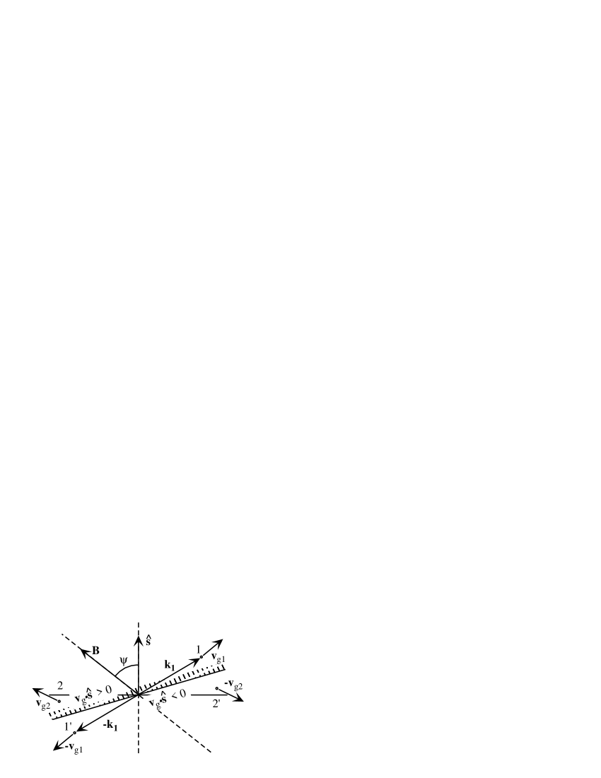
Figure 9: The $k$-space over which the flux integration should be carried is the region in which ${\bf v}_{g}\cdot\hat{{\bf s}}>0$ – i.e. , above the hatched line. Each point in the integration region (e.g. 1,2) has however a counterpart outside the region (1’,2’) for which the group velocity is opposite. If we integrate $|{\bf v}_{g}\cdot\hat{{\bf s}}|$ over all space we get twice the required answer without the complication arising from the boundary.

In our coordinate system, we have that the radial unit vector is:

$$\hat{\bf r}=\sin\theta\cos\phi\,\hat{\bf x}+\sin\theta\sin\phi\,\hat{\bf y}+\cos\theta\,\hat{\bf z}.$$ (42)

The unit vector in the direction of $\theta$ is needed for the group velocity, it is:

$$\hat{\bf\theta}=\cos\theta\cos{\phi}\,\hat{\bf x}+\cos\theta\sin\phi\,\hat{\bf y}-\sin\theta\,\hat{\bf z}.$$ (43)

Last, we need the vector in the direction normal to the surface element. If the angle between the magnetic field direction and the normal to the surface is $\psi$, then this vector is:

$$\hat{{\bf s}}=-\sin\psi\,\hat{\bf x}+\cos\psi\,\hat{\bf z}.$$ (44)

The group velocity is related to $\omega$ through:

$${\bf v}_{\hbox{\rm\scriptsize g}}=\nabla_{k}\omega=\left(\partial\omega\over\partial k\right)_{\theta}\,\hat{\bf r}-{1\over k}\left(\partial\omega\over\partial\theta\right)_{k}\,\hat{\bf\theta}.$$ (45)

If the index of refraction is in the form $n=1+f(B)\sin^{2}\theta$, then we find:

$${\bf v}_{\hbox{\rm\scriptsize g}}={1\over 1+f(B)\sin^{2}\theta}\,\hat{\bf r}-{2f(B)\sin\theta\cos\theta\over(1+f(B)\sin^{2}\theta)^{2}}\,\hat{\bf\theta}.$$ (46)

The integrand is therefore:

$$n^{3}\left|{\bf v}_{\hbox{\rm\scriptsize g}}\cdot\hat{{\bf s}}\right| = \left|\left(1+f(B)\sin^{2}\theta\right)^{2}\times\right.$$ (47)

$$\left.\left(\cos\psi\cos\theta-\sin\psi\sin\theta\cos\phi\right)\right.$$

$$\left.+2f(B)\sin\theta\cos\theta\left(1+f(B)\sin^{2}\theta\right)\times\right.$$

$$\left.\left(\sin\psi\cos\theta\cos\phi+\sin\theta\cos\psi\right)^{\phantom{1}}\hskip-4.0pt\right|.$$

Next, we need to integrate over the NS surface with its varying field strength and varying directions. Since we assume it to be a dipole, we have that if the equatorial magnitude of the magnetic field is $B_{\hbox{\rm\scriptsize eq}}$ then on the surface we have:

$${\bf B}=B_{\hbox{\rm\scriptsize eq}}\left(3(\hat{{\bf s}}\cdot\hat{\bf m})\hat{{\bf s}}-\hat{\bf m}\right).$$ (48)

We thus find that the magnitude of ${\bf B}$ and its angle from the local normal are:

$$B = \sqrt{3(\hat{{\bf s}}\cdot\hat{\bf m})^{2}+1}B_{\hbox{\rm\scriptsize eq}}=\sqrt{3\cos^{2}\alpha+1}B_{\hbox{\rm\scriptsize eq}}$$ (49)

$$\cos\psi = \hat{\bf B}\cdot\hat{{\bf s}}={2\cos\alpha\over\sqrt{3\cos^{2}\alpha+1}}.$$ (50)

We further use that $f(B)$ is linear in $B$ in the interesting regime, implying that $f(B)=f(B_{\hbox{\rm\scriptsize eq}})B\equiv f_{0}\sqrt{3\cos^{2}\alpha+1}$.

The growth of the effective area of the whole star can now be written as:

$${a^{\prime}\over a}={1\over a}\int da^{\prime}={1\over a}\int da{da^{\prime}\over da}={1\over 4\pi}\int d\Omega_{a}{da^{\prime}\over da},$$ (51)

where $\int d\Omega_{a}$ implies an integration over the surface colatitude and longitude $(\alpha,\varphi)$. The integration over $\phi$ is trivial and we have:

$${a^{\prime}\over a}\hskip-3.0pt = \hskip-3.0pt{1\over 4\pi}\int_{1}^{-1}d(\cos\alpha)\int_{1}^{-1}d(\cos\theta)\int_{0}^{2\pi}d\phi\times$$ (52)

$$\left|\left(1+f(B)\sin^{2}\theta\right)^{2}\left(\cos\psi\cos\theta-\sin\psi\sin\theta\cos\phi\right)\right.$$

$$\left.+2f(B)\sin\theta\cos\theta\left(1+f(B)\sin^{2}\theta\right)\right.\times$$

$$\left.\left(\sin\psi\cos\theta\cos\phi+\sin\theta\cos\psi\right)^{\phantom{1}}\hskip-4.0pt\right|,$$

where we explicitly have to express $f(B)$ as $f_{0}\sqrt{3\cos^{2}\alpha+1}$ and $\cos\psi$ as $2\cos\alpha/\sqrt{3\cos^{2}\alpha+1}$. The integration is nontrivial (mainly because of the absolute sign) but is however straight forward if done numerically. The method used was a Monte Carlo integration which easily achieved accuracies better than $10^{-3}$ for several dozen magnetic field strengths in roughly an hour of an HP workstation CPU time.

Another useful computation is the direct evaluation and the construction of a fitting formula for the local increase in the black-body flux as given by eq. 41. The integral is generally a nonlinear function of both the magnetic field strength $B$ and the angle $\psi$ between the magnetic field, ${\hat{\bf B}}$, and the surface normal, $\hat{{\bf s}}$. Thus, a simple fit can only be found in the limit of weak fields ($B\ll B_{0}\approx 1.13\times 10^{17}$ G), it is:

$$1+g(B,\psi){\hskip-4.0pt} \equiv {\hskip-4.0pt}{da^{\prime}\over da}\approx 1+\left(1+0.067\cos\psi+1.6024\cos^{2}\psi\right.$$ (53)

$$\left.-0.672\cos^{3}\psi\right)\left(B/B_{0}\right)$$

Its relative accuracy is better than $10^{-3}$, which is the integration accuracy.

References

- Adler 1971 Adler, S. L. 1971, Ann. Phys., 67, 599.
- Arzoumanian et al. 1994 Arzoumanian, Z., Nice, D. J., Taylor, J. H. & Thorsett, S. E. 1994, ApJ, 422, 671.
- Baring 1995 Baring, M. G. 1995, ApJL, 440, 69.
- Baring & Harding 1995 Baring, M. G. & Harding, A. K. 1995, Astrophys. Sp. Sci., 231, 77.
- Berestetskii, Lifshitz & Pitaevskii 1982 Berestetskii, V. B., Lifshitz, E. M. & Pitaevskii, L. P. 1982, Quantum Electrodynamics, Pergamon, Oxford, second edition
- Dittrich & Reuter 1985 Dittrich, W. & Reuter, M. 1985, Effective Lagrangians in quantum electrodynamics, Springer-Verlag, Berlin
- Erber 1966 Erber, T. 1966, Rev. Mod. Phys., 38, 626.
- Gold 1968 Gold, T. 1968, Nature, 218, 731.