The effective electron mass in core-collapse supernovae

Abstract

Finite temperature field theory is used to calculate the correction to the mass of the electron in plasma with finite temperature and arbitrary chemical potential, and the results are applied to the core regions of type II supernovae (SNe). It is shown that the effective electron mass varies between 1 MeV at the edge of the SN core up to 11 MeV near the center. This changed electron mass affects the rates of the electroweak processes which involve electrons and positrons. Due to the high electron chemical potential, the total emissivities and absorptivities of interactions involving electrons are only reduced a fraction of a percent. However, for interactions involving positrons, the emissivities and absorptivities are reduced by up to 20 percent. This is of particular significance for the reaction $\bar{\nu}+p\leftrightarrow e^{+}+n$ which is a source of opacity for antineutrinos in the cores of type II SNe.

1 Introduction

The properties of electrons are modified by the medium through which they propagate. In particular, the energy-momentum relation for electrons is changed from the well-known $E^{2}=p^{2}+m_{e}^{2}$ to a different relation. This change may be modeled by defining a momentum dependent effective electron mass, $m_{\rm eff}^{2}=E^{2}-p^{2}$, which replaces the vacuum mass of the electron in all calculations involving electrons and positrons. This has important astrophysical consequences.

The consequences of the effective mass of the electron has been the subject of much interest recently in the context of Big Bang Nucleosynthesis (BBN) (e.g. Chapman chapman (1997)). During BBN, plasma effects at temperatures of around 1 MeV lead to a small change in the effective electron mass, leading to modified neutron-proton transition rates. This in turn leads to a small change (generally less than 1 percent) in the abundance of light elements produced by BBN (Dicus dicus (1982); Sawyer sawyer (1996)). It is possible that consequences of such small changes in the early universe will have observable consequences with the advent of the next generation of cosmic microwave background satellites (Lopez and Turner lopez (1998)).

On the other hand, the implications of the change in electron mass at the higher temperatures and densities found in the cores of type II SNe remain unexplored. Typically, finite temperature calculations of relevance to BBN are carried out at zero chemical potential, as there are essentially similar numbers of electrons and positrons in the early universe. In the highly degenerate cores of core-collapse SNe this assumption breaks down, and the finite chemical potential effects must be included. The extension of existing theory to this regime is made here, where it is shown that the effective mass of the electron increases with increasing chemical potential, and that for the densities of relevance in the cores of type II SNe, the electron mass may be over 20 times its vacuum mass.

One might assume that an increase in the effective mass of the electron of this magnitude must have immediate drastic consequences for the physics of type II SNe, as the electron takes part in various processes important to the neutrino opacity in the core. This is not the case. While electrons play a significant role in the transport of neutrinos through the core of a SNe, generally the electron chemical potential is so high that Fermi blocking ensures that the electrons involved in neutrino reactions are ultra-relativistic. In this regime, the finite mass of the electron leads to a small correction to the rates in the ultra-relativistic limit. Increasing the electron mass increases this correction, but it remains relatively small.

On the other hand, the mass of the positron is also changed, and is essentially equal to the mass of the electron. As the positron reactions are not affected by Fermi blocking, the interaction rates involving positrons may be substantially modified. It is shown here that these corrections in the cores of SNe are of the order of 10 to 20 percent.

The basic interaction rates between neutrinos and nucleons, nuclei, electrons, and positrons have been known for many years (see the Appendices of Bruenn (bruenn (1985)) for a summary). More recently, the changes in these rates due to many body effects in the dense nuclear medium have been examined (e.g. Reddy et al. reddy (1998)). This has lead to a decrease in the total neutrino opacities, though the exact size of this decrease is still the subject of some theoretical uncertainty (Raffelt & Seckel raffelt (1995)). Here, a different effect is considered, that of finite temperature effects on the electrons in the medium.

A complete calculation of the lowest order finite temperature contributions to the neutrino absorption, emission and scattering rates in a SN core requires the inclusion of not just the modified electron mass, but also absorption of particles from the plasma, stimulated emission (which is Fermi blocking for fermions), and the use of finite temperature wave functions (Donoghue & Holstein donoghue (1983)). This last point is problematic, as there are technical difficulties in precisely describing the wave functions for massive particles in a medium (Chapman chapman (1997)), especially for the regime considered here, where the electron mass is many times its vacuum mass. There are essentially three prescriptions for the construction of finite temperature wave-functions in the literature (Donoghue & Holstein donoghue (1983); Sawyer sawyer (1996); Esposito et al. esposito (1998)), and there is some confusion as to which prescription is correct. Given this difficulty, this paper is restricted to a calculation of the effects due to the increased electron mass and Fermi blocking. Preliminary estimates based on the work of Sawyer (sawyer (1996)) suggest that these are the dominant effects.

The plan of this paper is as follows. In the following Section, the theory for calculating the electron mass at finite temperature and chemical potential is presented, then these forms are evaluated for the conditions expected within a core collapse SN. In Sec. 4, the modifications to both $\beta$-decay type reactions, and neutrino scattering off electrons and positrons are calculated. Finally, the conclusions of this work are drawn.

2 Electron mass

It has long been recognized that photons propagating in a plasma have behaviour quite different to those propagating in vacuo. These changes include a modified dispersion relation (due to a finite plasma frequency), the appearance of new modes, different polarization properties, and some momenta for which the photons cannot propagate. In fact, such effects apply to all particles, though the magnitude of the changes induced by a medium are dependent on the strength of the interactions between the particle and the medium. For instance, in the cores of type II supernovae, neutrons and protons (SNe) have effective masses different from their vacuum masses (Horowitz & Serot horowitz (1987)). Also, it is known that neutrinos acquire an induced mass in a medium allowing them to undergo resonant mixing (the MSW effect) (Mikheyev & Smirnov mikheyev (1985)). Similarly, the properties of electrons are modified by the medium through which they propagate, and this leads to a changed dispersion relation (i.e. an effective mass which is momentum dependent), and changed polarization properties (Weldon weldon (1982)).

The effective mass of the electron at finite temperature may be understood as an application of the optical theorem to electrons: an electron in a plasma acquires an energy momentum relationship different to that in vacuo due to forward scattering interactions with the photons and electrons in the plasma. Changing to the notation of Weldon (weldon (1982)), if the electron energy is $\omega$ and its momentum is $k$, the effective mass of the electron is then given by

$$m_{\rm eff}^{2}=\omega^{2}-k^{2}.$$ (1)

To lowest order in the fine structure constant, $\alpha$, the reactions that contribute to the effective mass of the electron are shown in Fig. 1a. These are just the diagrams for Compton scattering and Moller scattering. The physical content of this idea may be expressed more rigorously in the language of finite temperature field theory. In this theory, the correction of the electron mass comes about through finite temperature corrections to the electron self-energy diagram, shown in Fig. 1b.

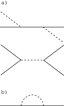
Figure 1: Lowest order Feynman diagrams representing the interactions which lead to the additional self-energy and hence the additional mass of the electron in a plasma.

A general procedure for calculating the one-loop correction to the electron mass was developed by Weldon (weldon (1982)). Weldon calculated the effective mass of massless fermions at finite temperature in the limit of high temperature with zero chemical potential for a variety of field theories. The procedure applicable to QED with finite electron mass was also outlined, and this method was applied by Donoghue and Holstein (donoghue (1983)), who gave approximate expressions for the electron mass at finite temperature and zero chemical potential. This expression was further approximated by Ahmed and Saleem (1987a ), who also extended their approximation to finite chemical potential (Ahmed & Saleem 1987b ).

The procedure outlined by Weldon (weldon (1982)) is followed here, allowing for arbitrary chemical potential. Initially, no approximation such as that used by Donoghue and Holstein (donoghue (1983)) are made, and this leads to some interesting observations concerning the nature of the collective modes of the electrons at low energy, such as the existence of a number of additional propagating modes at low momenta.

The correction to the mass of the electron may be calculated from the electron self-energy diagram shown in Fig. 1. In general, the self-energy, $\Sigma$, at finite temperature will be a linear combination of $K$, the 4-momentum of the electron, $u$, the 4-velocity of the background plasma, and $1$, the unit matrix. Thus, the self energy may be written,

$$\Sigma=-a/\!\!\!\!K-b/\!\!\!u-c^{\prime},$$ (2)

where $a$, $b$, and $c^{\prime}$ are functions of the Lorentz invariants

$$\omega=(K\cdot u),\qquad k=\left[(K\cdot u)^{2}-K^{2}\right]^{1/2},$$ (3)

which, in the frame of the background plasma, may be identified as the energy and momentum of the electron.

Now, including the correction for the self-energy, the electron propagator may be written,

$$S^{-1}=/\!\!\!\!K-m-\Sigma=(1+a)/\!\!\!\!K+b/\!\!\!u-c,$$ (4)

with $c=-c^{\prime}+m$. As discussed in Weldon (weldon (1982)), the energy-momentum relation for the propagating electron modes of the system are given by the location of the poles of the propagator. These poles are determined by the zeroes of the function

$$D(k,\omega)=(1+a)^{2}K^{2}+2(1+a)b(K\cdot u)+b^{2}-c^{2}=0,$$ (5)

and the propagator is given by

$$S=[(1+a)/\!\!\!\!K+b/\!\!\!u+c]/D.$$ (6)

If one defines

$$A=-{1\over 4}{\rm Tr}[/\!\!\!\!K\Sigma],\quad B=-{1\over 4}{\rm Tr}[/\!\!\!u\Sigma],\quad C=-{1\over 4}{\rm Tr}[\Sigma],$$ (7)

then using Eq. (2), one obtains,

$$a = {1\over k^{2}}(B\omega-A),$$

$$b = {(k^{2}-\omega^{2})B+\omega A\over k^{2}},$$

$$c^{\prime} = C.$$ (8)

The use of the one loop expression for $\Sigma$ in evaluating $A$, $B$, and $C$, then defines the constants in dispersion function, Eq. (5). The zeroes of this function may then be found, determining the electron energy-momentum relation and hence the effective mass of the electron.

To determine the above coefficients it is necessary to explicitly calculate the finite-temperature contribution to the electron self-energy. The algebraic form corresponding to the diagram shown in Fig. 1b may be written

$$\Sigma(K)=ie^{2}\int{d^{4}p\over(2\pi)^{4}}D_{\mu\nu}(p)\gamma^{\mu}S(p+K)\gamma^{\nu},$$ (9)

where the propagators used are finite temperature propagators given by

$$D_{\mu\nu}(p)=-g_{\mu\nu}\left[{1\over p^{2}+i0}-2\pi i\delta(p^{2})n_{b}(p)\right],$$ (10)

for the bosons, with $n_{b}(p)$ the boson occupation number, and

$$S(p)=(/\!\!\!p+m)\left[{1\over p^{2}-m^{2}+i0}+i{N(p)\over 2m}\right],$$ (11)

with $N(p)=\sum_{\epsilon=\pm}4\pi m\delta(p^{2}-m^{2})H(\epsilon p^{0})n^{\epsilon}(p)$, where $H$ denotes the Heaviside step function, and $n^{+}(p)$ and $n^{-}(p)$ are the electron and positron distribution functions, respectively. (Note $+$ denotes the particle, and $-$ denotes the antiparticle.)

One may shift the integration in the fermion term of Eq. (9) through $p\rightarrow p-K$, leading to

$$\Sigma(K) = 2e^{2}\int{d^{4}p\over(2\pi)^{4}}\left[{(2m-/\!\!\!p)N(p)\over 2m((p-K)^{2}+i0)}\right.$$ (12)

$$\left.\qquad-{(2m-/\!\!\!p-/\!\!\!\!K)2\pi\delta(p^{2})n_{b}(p)\over(p+K)^{2}-m^{2}+i0}\right],$$

where only term involving a single distribution function has been kept. (The term involving no distribution functions is the vacuum self energy of the electron, which is removed by renormalization, and the term involving two distribution functions is acausal, and thus not physical.) Writing

$$L_{1} = {\rm ln}\left[{2(\omega\varepsilon+kp)-K^{2}-m^{2}\over 2(\omega\varepsilon-kp)-K^{2}-m^{2}}\right],$$

$$L_{2} = {\rm ln}\left[{2(\omega\varepsilon+kp)+K^{2}+m^{2}\over 2(\omega\varepsilon-kp)+K^{2}+m^{2}}\right],$$

$$L_{3} = {\rm ln}\left[{2p(\omega+k)+K^{2}-m^{2}\over 2p(\omega-k)+K^{2}-m^{2}}\right],$$

$$L_{4} = {\rm ln}\left[{2p(\omega+k)-K^{2}+m^{2}\over 2p(\omega-k)-K^{2}+m^{2}}\right],$$ (13)

with $\varepsilon=(p^{2}+m^{2})^{1/2}$, one may perform three of the integrals in Eq. (12), leading to

$$A_{b} = -{e^{2}\over 16\pi^{2}k}\int_{0}^{\infty}dp\,n_{b}(p)\left[8kp\right.$$

$$\qquad\left.+(K^{2}+m^{2})(L_{3}-L_{4})\right]$$

$$A_{f} = -{e^{2}\over 16\pi^{2}k}\int_{0}^{\infty}{dp\,p\over\varepsilon}\left[4kp(n^{+}(p)+n^{-}(p))\right.$$

$$\qquad\left.+(K^{2}+m^{2})(n^{+}(p)L_{1}-n^{-}(p)L_{2})\right]$$

$$B_{b} = -{e^{2}\over 8\pi^{2}k}\int_{0}^{\infty}dp\,n_{b}(p)\left[(p+\omega)L_{3}-(p-\omega)L_{4}\right]$$

$$B_{f} = -{e^{2}\over 8\pi^{2}k}\int_{0}^{\infty}dp\,p\left[n^{+}(p)L_{1}+n^{-}(p)L_{2}\right]$$

$$C_{b} = {me^{2}\over 4\pi^{2}k}\int_{0}^{\infty}dp\,n_{b}(p)\left[L_{3}-L_{4}\right]$$

$$C_{f} = {me^{2}\over 4\pi^{2}k}\int_{0}^{\infty}{dp\,p\over\varepsilon}\left[n^{+}(p)L_{1}-n^{-}(p)L_{2}\right],$$ (14)

where the constants of Eq. (7) have been separated into boson and fermion contributions, according to the appearance or the relevant distribution function from Eq. (12). Eq. (14) reduces to the expressions given by Weldon (weldon (1982)) in the limit of zero electron mass and zero chemical potential (i.e. $n^{+}=n^{-}=n_{f}$). In the limit of zero chemical potential and making the same approximations, Eq. (14) reduces to that of Donoghue and Holstein (donoghue (1983)). Both of these results also reduce to that of Peressutti and Skagerstam (peressutti (1982)) in the limit of zero electron momentum.

To determine the electron mass at a given momentum, the electron dispersion relation, Eq. (5), must be solved numerically using Eq. (14). Rewriting Eq. (5) in terms of $A$, $B$, and $C$ through Eq. (8) leads to

$$A^{2}-2A(k^{2}+B\omega)+B^{2}K^{2}+k^{2}((C-m)^{2}-K^{2})=0,$$ (15)

with $A=A_{f}+A_{b}$, etc.

Integration over the logarithmic functions in Eq. (14) is complicated by the singularities caused by the zeros in the numerators and denominators. These zeros are located at

$$p_{1\pm}={(\omega\pm k)^{2}\mp m^{2}\over 2(\omega\pm k)},$$ (16)

for $L_{1}$ and $L_{2}$, and at $-p_{2\pm}$ for $L_{3}$ and $p_{2\pm}$ for $L_{4}$, with

$$p_{2\pm}={\omega^{2}-k^{2}-m^{2}\over 2(\omega\pm k)}.$$ (17)

In general, the coefficients $A$, $B$, and $C$ will be complex valued, as the arguments of the logarithms in Eq. (14) are negative for values of $p$ between the two zeros. The logarithms in Eq. (14) are to be taken in the principle value sense, and the imaginary part of the coefficients are neglected.

The approximations made by Donoghue & Holstein (donoghue (1983)) lead to the relation

$$m_{\rm eff}^{2}=m^{2}-2(A+mC)$$ (18)

which is obviously much simpler to evaluate than the solutions to Eq. (15), and, as is shown below, is quite accurate.

2.1 Reaction rates

To calculate reaction rates at finite temperature, it is necessary to use finite temperature spinors, which are the solutions of a modified Dirac equation, given by

$$(/\!\!\!\!K-m-\Sigma)U=0,$$ (19)

where U is the spinor wave function in the medium. For a massless electron, it was shown by Weldon (weldon (1982)) that the wave functions in the medium are unchanged in form from their vacuum counterparts – only their normalization is modified, and the normalization coefficient may be calculated by determining the residue of the electron propagator at the electron pole. Donoghue and Holstein (donoghue (1983)) considered finite temperature effects on the mass of a massive electron. In this case, in general, the solutions to Eq. (19) do not correspond to the vacuum solutions. Donoghue and Holstein made an assumption that a corresponding set of states did exist and calculated the normalization coefficient based on this assumption. The coefficient is given by

$$Z_{2}^{-1}=1-\left.(\omega+B)^{-1}\left(\omega+{\partial A\over\partial\omega}+m{\partial C\over\partial\omega}\right)\right|_{\omega=\sqrt{k^{2}+m^{2}}}.$$ (20)

Sawyer (sawyer (1996)) reexamined this procedure and made a perturbation series expansion around the vacuum poles of the propagator, effectively calculating the projection operators to be used within QED at finite temperature. Esposito et al. (esposito (1998)) also adopted a peturbative approach, but obtain a result different from both Sawyer and Donoghue and Holstein.

For this work, a further problem presents itself. As is shown below, electrons in the core of a SN may have masses many times their vacuum mass. Thus, it is unclear whether a perturbation series expansion around the vacuum poles of the propagator is a valid approach to this problem at all. In the absence of a well defined theory, it is assumed that wave-function renormalization effects are unimportant in comparison to the kinematical effects of the changed electron mass. It is unlikely that the correct inclusion of normalization effects will have a significant effect on the results presented, as, in the regime of interest, the high electron chemical potentials ensure that the electrons are relativistic. This implies that the vacuum mass of the electron is relatively unimportant, rendering the massless approach of Weldon (weldon (1982)), in which there are no normalization effects, approximately valid.

3 Evaluation of the effective mass

To evaluate the effective mass of the electron, the locations of the zeroes of the dispersion function, Eq. (15), must be found numerically. Assuming a plasma temperature of 1 MeV and a chemical potential of 10 MeV, the dispersion function as a function of particle energy is shown for a variety of electron momenta in Fig. 2. The point where these dispersion relations pass through the zero point identifies the energy of the particle for its given momentum.

Figure 2: Dispersion functions for electrons in a plasma with temperature of 1 MeV and chemical potential of 10 MeV, for a variety of electron momenta. The physical energy of the electron is given by the value of the abscissa for which the dispersion function is zero. Note that multiple roots appear at low momenta.

The structure of the dispersion functions in Fig. 2 is quite complicated, and shows that for low momenta there exist multiple roots to the electron dispersion equation. An effect analogous to this has been noted before by Klimov (klimov (1981)) and Weldon (weldon (1982), weldon89 (1989)), where two solutions to the electron dispersion relation at zero chemical potential and zero electron mass were found. These were identified as one root corresponding to the electron, and one to a propagating collective mode later labeled the “plasmino” by Braaten (1992). The second of the lower two roots at small momenta in Fig. 2 may be identified as the plasmino mode. The existence of the third zero in the dispersion equation of electrons at low momentum has not been noted before, due to the analytic approximations made in calculating the mode structure. Whether this zero corresponds to a propagating mode depends on the ratio of the imaginary part of the electron self-energy to the real part. If this ratio is comparable to or larger than unity then this mode is strongly damped and does not propagate.

While the structure of the electron dispersion relation, and the nature of these new modes are a fascinating subject in their own right, no analysis of the effects of these new modes will be made here. Given that they only appear at low momenta, they are unlikely to have a significant dynamical effect, as the relevant energy scales for electrons are the temperature and chemical potential, which are high. Attention is restricted to the electron-like pole of the electron dispersion relation, avoiding the difficult task of calculating the polarization and damping characteristics of these new modes. Note, however, that these new modes are of interest and should be investigated.

For a variety of values of chemical potential, the effective mass as a function of momentum is shown in Fig. 3. Also shown is the approximate form of the electron mass as given by Eq. (18). Clearly, this form is quite a good approximation to the electron-like pole of the dispersion function, and may be used for efficient evaluation of the effective electron mass at all chemical potentials.

Figure 3: Ratio of the effective electron mass to the vacuum electron mass as a function of electron momentum for various chemical potentials at a temperature of 1 MeV. The dashed line corresponds to the approximation of Donoghue and Holstein (1983).

For concreteness, a particular model for the central regions of a core-collapse SN as generated by S. Bruenn (bruenn (1985)) is now considered. The relevant data for this model is shown in Fig. 4. This model is based on a 15 solar mass progenitor around 0.2 seconds after core bounce. At this stage the bounce shock has proceeded to around 100 km and the semi-opaque region for the neutrinos lies between 10 to 50 km. The electron mass as a function of radius for this model is shown in Fig. 5. This effective mass was calculated for electrons with their momenta set at half the chemical potential of the plasma. This ensure the mass is within the flat region of the curves in Fig. 3, and is in the appropriate range for the reactions considered below.

Figure 4: Data from a numerical simulation of a SN by Bruenn.

Figure 5: The electron effective mass as a function of distance from the center of a type II SN.

3.1 Equilibria

The increase in the effective mass of the electron in the core regions of a supernova has an effect on the relative numbers of particles which form an equilibrium plasma in these dense environments. A detailed calculation of the equilibrium configurations of an ideal neutron, proton, electron and neutrino gas at fixed lepton fraction has been made both with and without the corrections to the electron mass. The corrections to the quantities characterizing the thermal equilibria, such as the chemical potentials of the electrons, protons, neutrons and neutrinos are of the order of $0.1$ percent, and are thus dynamically unimportant.

4 Reaction rates

The results of Sec. 3 are now applied to determine the change of neutrino opacities in the cores of SNe. In general, it might be argued that the electron mass effects should be great, as the standard correction to the neutrino scattering rates scales as $m_{e}^{2}/T^{2}$, which is of order 1 for the region near the center of the SN. However, for interactions involving degenerate distributions of electrons, the correction to the rate scales as $m_{e}^{2}/\mu_{e}^{2}$, which is always a small quantity in a SN. Thus only rates of interactions which involve positrons are significantly modified.

The changes to the absorptivity, $1/\lambda^{(a)}(\omega)$, for the processes $\nu_{e}+n\rightleftharpoons e+p$, $\bar{\nu}_{e}+p\rightleftharpoons e^{+}+n$, and $\nu_{e}+A^{\prime}\rightleftharpoons A+e$ as calculated by Bruenn (bruenn (1985)) are calculated. The approximate rates for these processes are given by

$$\nu_{e}+n \rightleftharpoons e+p:$$

$${1\over\lambda^{(a)}(\omega)} = {G^{2}\over\pi}\eta_{np}(g_{V}^{2}+3g_{A}^{2})\left[1-f_{e}(\omega+Q)\right]$$

$$\qquad\times(\omega+Q)^{2}\left[1-{m_{E}^{2}\over(\omega+Q)^{2}}\right]^{1\over 2};$$

$$\bar{\nu}_{e}+p \rightleftharpoons e^{+}+n:$$

$${1\over\lambda^{(a)}(\omega)} = {G^{2}\over\pi}\eta_{pn}(g_{V}^{2}+3g_{A}^{2})\left[1-f_{e+}(\omega-Q)\right]$$

$$\times\,(\omega-Q)^{2}\left[1-{m_{E}^{2}\over(\omega-Q)^{2}}\right]H(\omega-Q-m_{e});$$

(22)

$$\nu_{e}+A^{\prime} \rightleftharpoons A+e:$$

$${1\over\lambda^{(a)}(\omega)} = {G^{2}\over\pi}n_{A}\exp[\beta(\mu_{n}-\mu_{p}-Q^{\prime})]g_{A}^{2}$$ (23)

$$\qquad\times{2\over 7}N_{p}(Z)N_{h}(N)\left[1-f_{e}(\omega+Q^{\prime})\right]$$

$$\qquad\times\,(\omega+Q^{\prime})^{2}\left[1-{m_{E}^{2}\over(\omega+Q)^{2}}\right]^{1\over 2};$$

where $G$ is the Fermi constant, $\eta_{np}$ and $\eta_{pn}$ are the effective neutron and proton number densities, respectively, $Q=1.2935$ MeV is the difference between neutron and protons masses, $N_{p}$, and $N_{h}$ are the number of neutrons and neutron holes in the $1f_{7/2}$ and $1f_{5/2}$ levels, respectively, $Q^{\prime}$ is approximately the difference between the neutron and proton chemical potentials plus 3 MeV, and $n_{A}$ is the number density of particles with atomic weight $A$. Note that as absolute magnitudes of these rates are not needed for this calculation, detailed knowledge of many of these quantities is unnecessary. For further details, consult Bruenn (bruenn (1985)).

Including the changes in the nature of the electron at finite temperature and chemical potential leads to a number of changes in the above rates. First, the electron mass in Eqs. (LABEL:eq:8)-(23) must be replaced with the effective electron mass (at high momentum). Secondly, each rate obtains a factor from the normalization of the external electron line given in Eq. (20), which is neglected here. Finally, the conditions relating to the minimum neutrino energy at which the process occurs are changed, with Eq. (LABEL:eq:8) requiring an extra term limiting the process to reactions where the neutrino energy is higher than $Q-m_{eff}$.

The ratio of modified to unmodified absorptivities, integrated over a thermal neutrino spectrum, are shown in Fig. 6 as a function of radius from the center of the SN. Note that under local thermodynamic equilibrium, the absorptivities and emissivities differ only by a factor of a neutrino distribution function. Thus, for thermal neutrino spectra, the emissivities and absorptivities will be changed by the inclusion of the modified electron mass by the same amount, as the effective electron mass does not directly affect the neutrino distribution function. The top panel of Fig. 6 shows that the neutrino interactions with neutrons and nucleons remain largely unchanged by the change in the electron mass. This is because the high electron chemical potentials found in the core of the SN restrict the energy of the created electron to very high energies. At these energies, the electron mass is a smaller fraction of the electron energy, and thus the correction due to the finite mass of the electron is only a small correction to the rate.

The bottom panel of Fig. 6 shows that the absorptivities (and emissivities) of antineutrinos is reduced by a substantial amount. This is because the positrons are not restricted to high energies by Fermi blocking. This may be seen in more detail in Fig. 7, where the ratio of the absorptivities is shown as a function of neutrino energy. Clearly the absorptivity is reduced much more at low energy (and the cut off for absorption is at a higher energy in the modified case). This may also be significant in the region between 10 and 20 km in which the plasma is only partially opaque to neutrinos and some energy equilibration between the neutrinos and the stellar plasma occurs. Although the total reduction in the rates is smaller in this region, the change in the energy distribution of the antineutrinos may have an effect on the predicted spectrum of anti-neutrinos observable from a galactic supernova.

Figure 6: Change in emissivities and absorptivities as a function of radius for the three nucleon processes mentioned in the text. The top panel shows that neutrino absorption and emission on nucleons and nuclei are hardly suppressed at all. The bottom panel shows that in the high density regions of the proto-neutron star, the absorption and emission of antineutrinos by nucleons is suppressed by up to 20 percent

Figure 7: Change in the absorptivity of antineutrinos on protons in the central regions of the core as a function of energy (arbitrary vertical scale). The unmodified rate is the dashed line, and the rate modified by the changed electron mass is shown as the solid line. The effect of the additional effective mass are largest at low energies. The average energy of the neutrinos in this region is around 30 MeV.

4.1 Neutrino-electron scattering

The calculation of neutrino electron scattering rates including electron mass corrections is an involved process, and for the sake of brevity, the scattering kernels will not be reproduced here. The reader is referred to Schinder and Shapiro (schinder (1982)) Eq. (47), which is the form of the rate used here.

In Fig. (8) the ratio of rates with and without a modified electron mass for neutrino-electron scattering and neutrino-positron scattering are integrated over ingoing and outgoing thermal distributions of neutrinos as a function of radius from the center of a model SN. Again it is shown that the rates involving electrons are not changed substantially, but interactions with positrons are reduced by about 15 percent. This is not a dynamically important effect for models of type II SNe, as the number of positrons in the core is exponentially suppressed by the very large chemical potential.

While there is relatively little change in the total opacity of neutrinos to electrons caused by the increased effective electron mass, there could be important changes introduced in the neutrino spectrum due to the increased elasticity of the scatterings. This is due to the dominant role that neutrino electron scatterings play in the energy exchange between the neutrinos and the electrons in the semi–transparent region found at densities of around $10^{13}$ $\mbox{g cm}^{-3}$.

Figure 8: Change in scattering rates as a function of radius for neutrino scattering off electrons and positrons. The total neutrino-electron scattering cross-sections are only reduced by around 0.3 percent.

It is worth noting also that at temperatures of greater than 1 MeV, the efficiency of electron positron production by neutrinos is decreased by the increase in the electron mass. This may be of relevance to Gamma Ray Burst scenarios which rely on neutrino heating. Though this effect is not studied in detail here, we expect the reduction to only be a matter of a few percent at 1 MeV (as the chemical potentials are small compared to the temperature) though it will be significantly higher at higher temperatures. Alternately, the rate of energy deposition due to neutrino electron scattering could be increased due to the additional mass of the electron at high temperature.

5 Conclusions

It has been shown that electrons within the core regions of core collapse SNe behave as if they have a mass many times their vacuum mass. In particular, the effective electron mass varies from around 11 MeV in the central regions of the core, to 1 MeV at the edge of the core. The primary effect of this increased electron mass is the reduction of the antineutrino emissivity and absorptivity off protons by around 20 percent. A complete calculation of these rates to lowest order in the fine structure constant requires a finite temperature treatment of the radiative corrections to the rate of $\bar{\nu}_{e}+p\rightleftharpoons e^{+}+n$, including a complete description of the finite temperature wave function of an electron in these dense environments.

References

- (1) Ahmed, K., Saleem, S., 1987, Phys. Rev D 35, 1861
- (2) Ahmed, K., Saleem, S., 1987, Phys. Rev D 35, 4020
- (3) Braaten, E., 1992, ApJ 392, 70
- (4) Bruenn, S., 1985, ApJS 58, 758
- (5) Chapman, I.A., 1997, Phys. Rev. D 55, 6287
- (6) Dicus, D.A., Kolb, E.W., Gleeson, A.M., et al., 1982, Phys. Rev. D 26, 2694
- (7) Donoghue, J.F., Holstein, B.R., 1983, Phys. Rev. D 28, 340. erratum 1984, Phys. Rev. D 29, 3004
- (8) Esposito, S., Mangano, G., Miele, G., Pisanti, O., 1998, hep-ph/9805428
- (9) Horowitz, C.J., Serot, B.D., 1987, Nucl. Phys. A 464, 613
- (10) Klimov, V.V., 1981, Sov. J. Nucl. Phys. 33, 934
- (11) Lopez, R.E., Turner, M.S., 1998, astro-ph/9807279
- (12) Mikheyev, S.P., Smirnov, A.Yu., 1985, Sov. J. Nucl. Phys. 42, 913
- (13) Peressutti, G., Skagerstam, B.S., 1982, Physics Letters B 110, 406
- (14) Raffelt, G., Seckel, D., 1995, Phys. Rev. D 52, 1780
- (15) Reddy, S., Prakash, M., Lattimer, J.M., Pons, J.A., 1998, astro-ph/9811294
- (16) Sawyer, R.F., 1996, Phys. Rev. D 53, 4232
- (17) Schinder, P.J., Shapiro, S.L., ApJS 50, 23
- (18) Weldon, H.A., 1982, Phys. Rev. D 26, 2789
- (19) Weldon, H.A., 1982, Phys. Rev. D 40, 2410