The Optical-Infrared Colour Distribution of a Statistically-Complete Sample of Faint Field Spheroidal Galaxies

Abstract

In hierarchical models, where spheroidal galaxies are primarily produced via a continuous merging of disk galaxies, the number of intrinsically red systems at faint limits will be substantially lower than in “traditional” models where the bulk of star formation was completed at high redshifts. In this paper we analyse the optical–near-infrared colour distribution of a large flux-limited sample of field spheroidal galaxies identified morphologically from archival Hubble Space Telescope data. The $I_{814}-HK^{\prime}$ colour distribution for a sample jointly limited at $I_{814}<$23 mag and $HK^{\prime}<$19.5 mag is used to constrain their star formation history. We compare visual and automated methods for selecting spheroidals from our deep HST images and, in both cases, detect a significant deficit of intrinsically red spheroidals relative to the predictions of high-redshift monolithic collapse models. However the overall space density of spheroidals (irrespective of colour) is not substantially different from that seen locally. Spectral synthesis modelling of our results suggests that high redshift spheroidals are dominated by evolved stellar populations polluted by some amount of subsidiary star formation. Despite its effect on the optical-infrared colour, this star formation probably makes only a modest contribution to the overall stellar mass. We briefly discuss the implications of our results in the context of earlier predictions based on models where spheroidals assemble hierarchically.

1 INTRODUCTION

The age distribution of elliptical galaxies is a controversial issue central to testing hierarchical models of galaxy formation. The traditional viewpoint (Baade 1957, Sandage 1986) interprets the low specific angular momentum and high central densities of elliptical galaxies with their dissipationless formation at high redshift. In support of this viewpoint, observers have cited the small scatter in the colour-magnitude relation for cluster spheroidals at low redshifts (Sandage & Visvanathan 1978, Bower et al 1992) and, more recently, such studies have been extended via HST imaging to high redshift clusters (Ellis et al 1997, Stanford et al 1997). Examples of individual massive galaxies with established stellar populations can be found at quite significant redshifts (Dunlop 1997).

In contrast, hierarchical models for the evolution of galaxies (Kauffmann et al 1996, Baugh et al 1996) predict a late redshift of formation for most galactic-size objects because of the need for gas cooling after the slow merger of dark matter halos. These models propose that most spheroidal galaxies are produced by subsequent mergers of these systems, the most massive examples of which accumulate since $z\simeq$1. Although examples of apparently old ellipticals can be found in clusters to quite high redshift, this may not be at variance with expectations for hierarchical cold dark matter (CDM) models since clusters represent regions of high density where evolution might be accelerated (Governato et al 1998). By restricting evolutionary studies to high density regions, a high mean redshift of star formation and homogeneous rest-frame UV colours would result; such characteristics would not be shared by the field population.

Constraints on the evolution of field spheroidals derived from optical number counts as a function of morphology (Glazebrook et al 1995, Im et al 1996, Abraham et al 1996a) are fairly weak, because of uncertainties in the local luminosity function. Nonetheless, there is growing evidence of differential evolution when their properties are compared to their clustered counterparts. Using a modest field sample, Schade et al (1998) find a rest-frame scatter of $\delta(U-V)$=0.27 for distant bulge-dominated objects in the HST imaging survey of CFRS/LDSS galaxies, which is significantly larger than the value of $\simeq$0.07-0.10 found in cluster spheroidals at $z\simeq$0.55 by Ellis et al 1997. Likewise, in their study of a small sample of galaxies of known redshift in the Hubble Deep Field (HDF), Abraham et al (1998) found a significant fraction ($\simeq$40%) of distant ellipticals showed a dispersion in their internal colours indicating they had suffered recent star formation possibly arising from dynamical perturbations.

Less direct evidence for evolution in the field spheroidal population has been claimed from observations which attempt to isolate early-type systems based on predicted colours, rather than morphology. Kauffmann et al (1995) claimed evidence for a strong drop in the volume density of early-type galaxies via a $V/V_{max}$ analysis of colour-selected galaxies in the Canada-France Redshift Survey (CFRS) sample (Lilly et al 1995). Their claim remains controversial (Totani & Yoshii 1998, Im & Castertano 1998) because of the difficulty of isolating a robust sample of field spheroidals from $V-I$ colour alone (c.f. Schade et al 1998), and the discrepancies noted between their analyses and those conducted by the CFRS team.

In addition to small sample sizes, a weakness in most studies of high redshift spheroidals has been the paucity of infrared data. As shown by numerous authors (eg. Charlot & Silk 1994), near-IR observations are crucial for understanding the star formation history of distant galaxies, because at high redshifts optical data can be severely affected by both dust and relatively minor episodes of star-formation. Recognizing these deficiencies, Moustakas et al (1997) and Glazebrook et al (1998) have studied the optica-infrared colours of small samples of of morphologically-selected galaxies. Zepf (1997) and Barger et al (1998) discussed the extent of the red tail in the optical-IR colour distribution of HDF galaxies. Defining this tail ($V_{606}$-$K>$7 and $I_{814}$-$K>$4) in the context of evolutionary tracks defined by Bruzual & Charlot’s (1993) evolutionary models, they found few sources in areas of multicolour space corresponding to high redshift passively-evolving spheroidals.

The ultimate verification of a continued production of field ellipticals as required in hierarchical models would be the observation of a decrease with redshift in their comoving space density. Such a test requires a large sample of morphologically-selected ellipticals from which the luminosity function can be constructed as a function of redshift. By probing faint in a few deep fields, Zepf (1997) and Barger et al (1998) were unable to take advantage of the source morphology; constraints derived from these surveys relate to the entire population. Moreover, there is little hope in the immediate term of securing spectroscopic redshifts for such faint samples. The alternative adopted here is to combine shallower near-infrared imaging with more extensive HST archival imaging data, allowing us to isolate a larger sample of brighter, morphologically-selected spheroidals where, ultimately, redshifts and spectroscopic diagnostics will become possible. Our interim objective here is to analyse the optical-infrared colour distribution of faint spheroidals which we will demonstrate already provides valuable constraints on a possible early epoch of star formation.

A plan of the paper follows. In $\S$2.1 we discuss the available HST data and review procedures for selecting morphological spheroidals from the images. In $\S$2.2 we discuss the corresponding ground-based infrared imaging programme and the reduction of that data. The merging of these data to form the final catalogue is described in $\S$2.3. In $\S$3 we discuss the optical-infrared colour distribution for our sample in the context of predictions based on simple star formation histories and consider the redshift distribution of our sample for which limited data is available. We also examine constraints based on deeper data available within the Hubble Deep Field. In $\S$4 we summarise our conclusions.

2 CONSTRUCTION OF THE CATALOGUE

2.1 THE HST SAMPLE

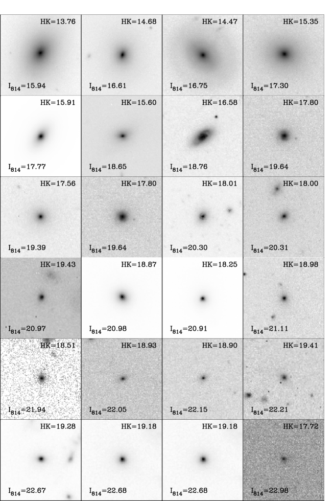
Figure 1: A selection of visually-classified spheroidal galaxies sorted by $I_{814}$ magnitude, selected from the HST archive. Each panel represents 10 arcsec on a side.

In searching the HST archive for suitable fields, we adopted a minimum $I$ F814W-band exposure time of 2500 sec and a Galactic latitude of $|b|$=19^∘ so that stellar contamination would not be a major concern. These criteria led to 48 fields accessible from the Mauna Kea Observatory comprising a total area of 0.0625 deg²(225 arcmin²). Table 1 lists the fields adopted, including several for which limited redshift data is available e.g. the HDF and its flanking fields (Williams et al 1996), the Groth strip (Groth et al 1994) and the CFRS/LDSS survey fields (Brinchmann et al 1997). F606W imaging is available for 25 of the fields in Table 1. Object selection and photometry for each field was performed using the SExtractor package (Bertin & Arnouts 1996). Although the detection limit varies from field to field, the $I_{814}$ -band data is always complete to $\sim 24$ mag and the $V_{606}$ -band to $\sim 25$ mag.

The morphologies of galaxies in the sample were investigated independently using visual classifications made by one of us (RSE), and automated classifications based on the central concentration ($C$) and asymmetry ($A$) parameters defined in Abraham et al. (1996b). In the case of visual classifications we adoped the MDS scheme defining spheroidal to include E: E/S0: S0 and S0/a (MDS types 0,1,2). As shown below, the visual and automated classifications compare quite favourably, with particularly satisfactory agreement for the regular spheroidal galaxies that are the focus of this paper.

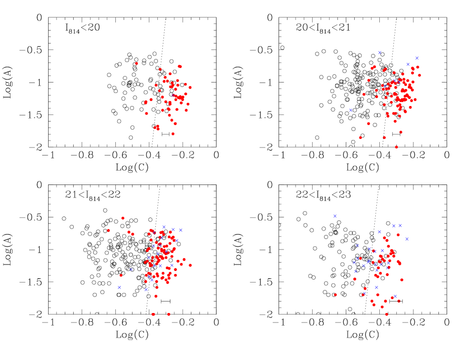
Figure 2: The distribution of asymmetry and concentration for visually-classified galaxies a) [top left] $I_{814}$ $<20$ mag, b) [top right] 20$<$$I_{814}$ $<$21 mag, c) [bottom left] 21$<$$I_{814}$ $<$22 mag (the limit achieved with the Medium Deep Survey) and (d) [bottom right] 22$<$$I_{814}$ $<$23 mag. The dashed lines represent optimal boundaries for the separation of spheroidal galaxies (solid circles) from spirals and irregulars (open circles). Compact objects are shown as crosses. The reference boundary line is defined using the visually identified sample at $I_{814}$ $<$20 and then shifted slightly as a function of magnitude on the basis of simulations. The expected 1$\sigma$ RMS errors on measures of central concentration are shown by the error bar on the lower right portion of each panel.

The appropriate limiting magnitude of our survey is set by that at which we believe we can robustly isolate spheroidal galaxies from compact HII galaxies, stars and bulge-dominated spirals. The Medium Deep Survey (MDS) analyses adopted a limiting magnitude for morphological classification (using nine classification bins) of $I_{814}$ =22 mag, although some MDS papers extended this further to $I_{814}$ =23 mag (see Windhorst et al 1996 for a summary). In Abraham et al (1996b) and Brinchmann et al (1997), HST data similar to that in the present paper was also used to classify galaxies to $I_{814}$ =22 mag. However, by restricting our analysis in the present paper to spheroidal systems, we are able to extend classifications to slightly deeper limits ($I_{814}$ =23.0 mag). This is possible because the chief diagnostic for discriminating spheroidals is central concentration, rather than asymmetry which is sensitive to lower surface brightness features. Because the classifications based on $A$ and $C$ are objective, the classification limits for the present dataset have been investigated using simulations, as described below.

Figure 1 shows a typical set of morphologically-identified spheroidals at various magnitudes down to $I_{814}$ =23 mag. Figure 2 compares the $A-C$ and visual morphological distributions at a range of magnitude intervals, down to the limits of our survey. The demarcation between early and late-types on the basis of $A$ and $C$ is made using bright galaxies ($I_{814}$ $<20$ mag) and shifted slightly as a function of magnitude on the basis of simulations made using the IRAF package artdata, which model the apparent change in the central concentration of an $r^{1/4}$ law elliptical galaxy as a function of decreasing signal-to-noise. Random errors on central concentration are also determined on the basis of simulations, and representative error bars are shown in Figure 2. The general agreement between the visual and automated classifications is remarkably good, particularly to $I_{814}$ $=$22 mag. Between $I_{814}$ $=$22 and 23 mag the agreement worsens, mostly because of the great increase in the number of visually-classified “compact” systems. We define compacts to be those systems where there is no clear distinction between small early-type galaxies, faint stars and/or HII regions.

In order to quantify the concordance between the visual and automated classifications, the $A-C$ distribution was analysed using a statistical bootstrap technique (Efron & Tibshirani 1993). The $A-C$ distribution was resampled 500 times in order to determine the uncertainties in both the number of systems classified as early-type, and the uncertainties on the colour distribution for these systems. These measurements will be discussed further below in §3.3.

The somewhat larger number (323 vs 266) of $A/C$-classified early-types relative to the visually classified galaxies is significant at the 3$\sigma$ level. However, if the compact systems are included in the tally of visually classified early-type systems, then the number of visually and A/C classified ellipticals agree closely (to within 1 sigma). It is clear that the distinction between compact galaxies and early-type systems is an important consideration when determining the number counts of early type systems at the faint limits of these data. However, it is perhaps worth noting at this stage that another bootstrap analysis (presented in §3.3) shows that the uncertainty introduced by compact systems into the number counts at $22<I<23$ does not manifest itself as a large uncertainty in the colour histograms of the early-type population.

2.2 GROUND-BASED INFRARED IMAGING

Although some of the fields in Table 1 have $V_{606}$ and $I_{814}$ HST data, such a wavelength baseline is not very useful at thesed depths. As discussed by Moustakas et al (1997) and Zepf (1997), the addition of infrared photometry is especially helpful in distinguishing between passively-evolving systems and those undergoing active star formation, regardless of redshift, primarily because of its reduced sensitivity to K-dimming, small amounts of star formation and dust reddening.

Our infrared imaging was mainly conducted using the QUIRC 1024² infrared imager on the University of Hawaii 2.2-m telescope. The log of observations is summarised in Table 2. In order to improve the observing efficiency in securing deep infrared photometry for a large number of WFPC-2 fields, we used the notched $H+K^{\prime}$ 1.8$\mu$m filter (which we refer to hereafter as the $HK^{\prime}$ filter) (Wainscoat & Cowie 1998, Figure 3) which offers a gain in sensitivity of typically a factor of $\simeq$2 over a conventional $K^{\prime}$ filter. At the f/10 focus of the UH 2.2m, the field of view is $193^{\prime\prime}\times 193^{\prime\prime}$ with a scale of $0.1886^{\prime\prime}\,$pixel^-1 ensuring that the 3 WFPC2 chips can be comfortably contained within a single exposure.

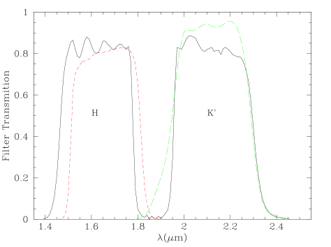
Figure 3: Transmission curve for the notched $HK^{\prime}$ filter(solid line) compared with that for the standard $H$ (dashed line) and $K^{\prime}$ (long-dashed line) passbands

Each $HK^{\prime}$ exposure was composed of 13 sub-exposures of $\simeq$100 sec duration (depending on the background level) spatially-shifted by increments of 5-20 arcsec in all directions. This dithering pattern was repeated 2-3 times during the exposure. The data was processed using median sky images generated from the disregistered exposures and calibrated using the UKIRT faint standards system. Most of the data was taken under photometric conditions; deep non-photometric data was calibrated via repeated short exposures taken in good conditions. The limiting magnitude of the infrared data varies slightly from field to field and is deepest for the HDF and flanking fields which were taken in a separate campaign (Barger et al 1998).

Figure 4: Statistical completeness of the UH 2.2m QUIRC data for the HST archival fields and the HDF as determined by procedures described in the text.

In order to determine the detection limit of our $HK^{\prime}$ data we performed extensive Monte Carlo simulations. Using the IRAF artdata package we created simulated data sets, which were subsequently analysed using the same extraction and measurement methods as for the real data. With the task mkobjects we generated artificial galaxies assuming exponential disk profiles with no internal absorption for spirals and de Vaucouleurs profiles for spheroidals. The profile scales were chosen to be magnitude-dependent converging to the image seeing at faint limits. Figure 4 shows the results of this exercise. The 80% completeness limit for spheroidals is $HK^{\prime}$=19.5 mag for most of the survey extending to $HK^{\prime}$=20.5 mag for the HDF and flanking fields.

2.3 COMPLETENESS OF THE COMBINED OPTICAL-INFRARED CATALOGUE

The final photometric catalogue of spheroidals was obtained by matching the HST $I_{814}$-band and the ground-based IR SExtractor catalogues using the adopted magnitude limits of $HK^{\prime}<$19.5 mag and $I_{814}$ $<$23.0 mag. In the final matched catalogue, we retained the SExtractor ‘$m_{best}$’ magnitudes but measured $I-HK^{\prime}$ colours within a fixed 3 arcsec diameter. This aperture size, together with the fairly good seeing of the IR data, ensures that when calculating colours we are looking at the same physical region of the galaxy. Of the 818 sources in the matched catalogue, 266 systems were visually classified as spheroidals (defined to be one of ‘E, E/S0, S0, or S0/a’ in the MDS scheme) and 50 as compact objects. Automated classifications result in 323 sources classed as spheroidals (with no distinction between spheroidals and compacts).

Clearly the joint selection by $I_{814}$ and $HK^{\prime}$ necessary to exploit HST’s morphological capabilities and establish optical-infrared colours could lead to complications when interpreting $I-HK^{\prime}$ colour distributions. As a major motivation for this study is to identify as completely as possible the extent of any red tail in the colour distribution, incompleteness caused by the various magnitude limits is an important concern. Figure 5 shows that, within the optical, morphologically-selected sample with $I_{814}$ $<$23 mag, virtually all of the $HK^{\prime}<$19.5 mag sample can be matched; only a small fraction (18/818=2.2%) of red $I-HK^{\prime}>$3.5-5 mag objects are missed. We return to the nature of these sources in $\S$3.3.

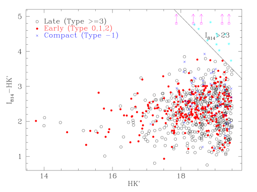
Figure 5: Colour-magnitude distribution for the visually-classified catalogue limited at $HK^{\prime}$=19.5 mag and $I_{814}$ =23 mag. Solid points correspond to spheroidals, crosses to compacts and circles to the remaining spirals and late type galaxies. The joint selection in $I_{814}$ and $HK^{\prime}$ implies a small fraction ($<$3%) of $HK^{\prime}$-selected objects are not contained within the HST sample. These objects are shown as stars and arrows as lower limit when no detection was possible

3 ANALYSIS

3.1 Strategy

Our analysis is motivated by the two principal differences we might expect between models where ellipticals underwent a strong initial burst of activity with subsequent passive evolution (which we will term the ‘monolithic collapse’ model) and those associated with a hierarchical assembly of ellipticals from the dynamical merger of gas-rich disks (Baugh et al 1996). We recognise at the outset that these models represent extreme alternatives with a continuum of intermediate possibilities (c.f. Peacock et al 1998; Jimenez et al. 1998). Our strategy in this paper, however, will be to discuss our field elliptical data in the context of the simplest models proposed to explain the star formation history of distant cluster ellipticals (Ellis et al 1997, van Dokkum et al 1998). More elaborate analyses are reserved until spectroscopic data is available for a large sample.

Firstly, in the monolithic collapse model, the comoving number density of luminous ellipticals should be conserved to the formation redshift (say, $z\simeq$3-5), whereas in hierarchical models we can expect some decline in number density at moderate redshift depending on the cosmological model and other structure formation parameters (Kauffmann et al 1996, Kauffmann & Charlot 1998a). Such a change in the absolute number density would be difficult to convincingly detect without spectroscopic data. The number of faint HST-identified ellipticals has been discussed by Glazebrook et al (1995), Driver et al (1995), Abraham et al (1996b) and Im et al (1996) with fairly inconclusive results because of uncertainties arising from those in the local luminosity function used to make predictions (Marzke et al 1998).

Secondly, there will be a redshift-dependent colour shift associated with merger-driven star formation in the hierarchical models whereas, for the monolithic case, the sources will follow the passive evolution prediction. Kauffmann et al (1996) initially claimed that both signatures would combine in the hierarchical picture to produce a factor 3 reduction in the abundance of passively-evolving sources by $z\simeq$1, but a more recent analysis (Kauffmann & Charlot 1998b) shows that the decline is dependent on the input parameters. For example in a model with non-zero cosmological constant (the so-called ’$\Lambda$CDM’), little decline is expected until beyond z$\simeq$1.

In contemplating these hypotheses in the context of our HST data, it must be remembered that although HST can be used very effectively to isolate spheroidals morphologically to $I_{814}$ =23 mag (representing a considerable advance on earlier colour-selected ground-based samples which could be contaminated by dusty later types), in the case of merger models, the predictions will depend critically on the time taken before a system becomes a recognisable spheroidal. However, any hypothesis which postulates a constant comoving number density of well-established spheroidals is well suited for comparison with our data, the outcome being important constraints on the past star formation history and luminosity evolution.

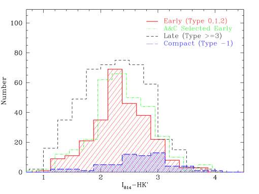
Figure 6: Colour histograms for various morphological samples within our adopted limits of $HK^{\prime}<$19.5 and $I_{814}$ =23. The solid line refers to the visually-classified spheroidals (MDS types 0,1,2) and the dashed-dot line to those spheroidals identified on the basis of their asymmetry and concentration indices. The long dashed line refers to visually-classed compacts (type=-1) and the short dashed line refers to the remainder (types $\geq$3).

3.2 Colour Distributions

Figure 6 shows $I_{814}$ -$HK^{\prime}$ colour histograms for both the visual and A/C-selected spheroidals alongside those for the compacts and the remainder. The automated and visual catalogues have nearly identical colour distributions, confirming earlier tests on the reliability of the automated classifier. In fact, the differences between the automated and visually defined histograms are almost completely attributable to the compact systems, which cannot be segregated from other early-types on the basis of central concentration. The colour histogram for compacts spans the range seen for early-type galaxies, with a peak slightly redward of that for visually classified early-types. It is clear from the similarity between the colour histograms for visual and automated classifications that contamination of spheroidals by compacts (expected in the automated catalogue) does not pose a significant uncertainty in determining the colour distribution.

The histogram of colours for late-type galaxies peaks at nearly the same colour as that for the early-types, which at first seems somewhat surprising. As we will later see, this is largely a reflection of the very wide redshift range involved. However, the distribution for spirals and later types is skewed toward the blue, although redward of $I-HK^{\prime}=$2.5 mag the shapes of the distributions are similar (see also §3.5 below).

3.3 Single Burst Model Predictions

Figure 7 compares the observed colour histograms with a range of model predictions based on the GISSEL96 spectral synthesis code (Bruzual & Charlot 1996) for a range of star-formation histories. Observed and predicted total counts for each of the models are also given in Table 3. At this stage we concentrate on ‘single burst’ or ‘monolithic collapse’ models which conserve the comoving number density at all epochs, and defer discussion of alternative scenarios until §3.5.

Our model predictions take into account the joint $I_{814}$ and $HK^{\prime}$ selection criteria for our sample, and are based on the present-day optical E/S0 luminosity function (LF) from Pozzetti et al. (1996), ie. a standard Schechter function with $\phi^{\star}=0.95\times 10^{-3}$ Mpc^-3, $M^{\star}_{b_{j}}=-20.87$ and a faint-end slope of $\alpha=-0.48$. When making model predictions, this luminosity function is tranformed into one appropriate for the $I_{814}$ photometric band via a single colour shift, resulting in $M^{\star}_{I_{814}}=-23.12$. For comparison, we also show predictions assuming a suitably transformed luminosity function with a flat faint-end slope ($\alpha=-1$) and $\phi^{\star}=0.55\times 10^{-3}$Mpc^-3 as suggested by Marzke et at (1998). Throughout this paper we adopt $H_{0}=50$ Km s^-1Mpc^-1. Given the elementary nature of the comparisons currently possible, and the fact that the expected dispersion in $I-HK^{\prime}$ from the present-day colour-luminosity relation is minimal, we have avoided the temptation to model a distribution of metallicities within the galaxy population, preferring instead to explore the effects of fixing the metallicity of the entire population to a single value within a large range (40%-250% solar) in the simple predictions discussed below. Other variables in the single burst hypothesis include the redshift of formation, $z_{F}$ (fixed at $z_{f}=5$), the burst-duration (represented as a top hat function of width 1.0 Gyr) and the cosmological parameters ($\Omega_{M}$ and $\Omega_{\Lambda}$). As shown in Appendix A, the luminosity weighted metallicities of the present sample are not biased strongly by the limiting isophotes of the our observations, and fair comparisons can be made using individual single-metallicity tracks over a broad range of redshifts.

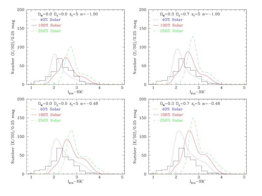
Figure 7: The colour distribution of visually-classified spheroidals with various single burst models (see legend) compared to the observed number, represented by solid histogram (see text for further assumptions).

Clearly the most important input parameter in the model predictions shown in Figure 7 (summarized in Table 3) is the metallicity. Although our spheroidals are almost exclusively luminous ($>L^{\ast}$) galaxies which, in the context of single-burst models would imply a metallicity of at least solar (cf. Appendix A, and Arimoto et al 1997), here we will explore the possibility that part of the colour distribution could arise from a wider metallicity range than that found locally.

3.3.1 A Deficit of Red Spheroidals

The predicted colour distributions show a characteristic asymmetry. This is caused by the blending of the $I_{814}-HK^{\prime}$ K-correction and the passive bluing of systems to $z\simeq$1.5. In contrast, the observations reveal a clear excess of blue ($I_{814}$ $-HK^{\prime}<$2 mag) spheroidals not predicted by even the lowest metallicity models. More significantly, solar and super-solar metallicity models over-predict the extent of the red tail in the colour distribution. Both discrepancies are consistent with recent star-formation in our sample of faint spheroidals. In order to quantify these discrepancies, we performed a Kolmogorov-Smirnov test (K-S) to check whether the observed spheroidal colours could be drawn from any of the model distributions (allowing a measurement error $\sigma_{I-HK^{\prime}}=0.25$ mag). In all cases the observed distribution differs from the models at a confidence level higher than 99.99%. Evidently monolithic collapse models with constant co-moving density fail to reproduce the colour distribution of high redshift spheroidals.

It will be convenient in the following to quantify the strength of the red tail in the colour distribution by defining a “red fraction excess”, shown in Table 3, constructed as the ratio of the predicted number of early type systems with $I_{814}-HK^{\prime}>3.0$ mag to the observed number. The statistical uncertainties on the red fraction excess in this table are based on 500 bootstrap resamplings of the original catalogue, each realization of which was subjected to the same selection criteria applied to the original data.

As discussed by many authors (Glazebrook et al 1995, Marzke et al 1998), the absolute numbers depends sensitively on the normalisation and shape of the local LF. Table 3 includes a summary for the range in LF parameters discussed earlier. For a declining faint-end slope ($\alpha=-0.48$) and solar-and-above metallicity, the red fraction excess is more than 5 times that observed. Adopting a metallicity substantially below solar results in closer agreement but assuming such metallicities for the entire population may be unreasonable given local values (see Appendix, and Arimoto et al 1997). Even so, the red fraction excess is only reduced from $\sim 8$ to $\sim 3$ if the adopted metallicity is varied between 250% solar and 40% solar. Models with a flat faint-end slope ($\alpha=-1$) improve the agreement further and in the very lowest metallicity model with $\Omega_{M}=0$ there is almost no deficit.

In Table 3 we have also included models with $\Omega_{\Lambda}>0$ for both slopes of the LF. The effect of $\Omega_{\Lambda}$ is to increase the apparent deficit of red spheroidals (because of the rapid increase in the differential volume element with redshift for $\Omega_{\Lambda}>0$ cosmologies at $z<1$).

Although models where the redshift of the initial burst, $z_{F}$, is reduced to $z=3$ are not shown in the table, these do not result in significant changes in the above discussions. We conclude that we cannot reconcile the number of galaxies in the red end of the observed colour histogram to the corresponding predictions of a constant co-moving density high-redshift monolithic collapse model. Alternative scenarios, which may explain the relatively blue colours of some observed spheroidals, will be considered in §3.5.

3.3.2 A Declining Number of High Redshift Spheroidals?

While monolithic collapse models fail to reproduce the observed colour distributions, Table 3 indicates that the overall number is in reasonable agreement. Specifically, for a low $\Omega_{M}$ and $\Omega_{\Lambda}$=0, the Marzke et al. luminosity function and luminosity-weighted metallicities of solar and above, we see no significant evolution in the space density of spheroidals. For the currently popular spatially-flat universe with low $\Omega_{M}$ and high $\Omega_{\Lambda}$ (Perlmutter et al 1999), the data imply a deficit of no more than 30%. Stronger evolution ($\sim$ 60% decline) would occur if we adopted the Pozetti et al. luminosity function. We therefore conclude that the colour offset described earlier is more likely the result of star-formation activity in well-formed spheroidals at high redshifts rather than evidence for evolution in their space density.

At this point, we return to the nature of those 18 sources identified in the infrared images which are fainter than $I_{814}$ =23 mag. Although they could formally be included in the colour distributions, they are too faint in the WFPC-2 images for reliable morphological classification. A montage of these sources is shown in Figure 8. At most 3 of the 18 are possible spheroidals. As such, their addition to the colour distribution would have a negligible impact on conclusions drawn from Figure 7.

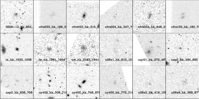
Figure 8: A montage of WFPC-2 images for those red sources contained within the $HK^{\prime}<$19.5 sample but for which $I_{814}$ $>$23.

3.4 Constraints from Redshift Distributions

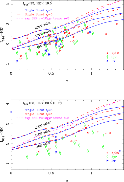
Figure 9: The colour-redshift relation for that subset of the $HK^{\prime}<$19.5 mag sample with published spectroscopic data (large symbols), and for a deeper $HK^{\prime}<$20.5 mag sample within the HDF for which photometric redshift data (smaller symbols) is available (Wang et al 1998). Symbols refer to visual classifications. The solid lines represents a passively evolving elliptical (single burst of duration 0.1 Gyr) at $z_{F}$=5 for different metallicities. Dashed lines show the corresponding models for $z_{F}$=3. Dot-dashed lines represent an exponential star formation with e-folding time $\tau=12$Gyr, truncated at $z=$3, with solar metallicity

While our principal conclusions are based on the enlarged size of our HST sample and addition of infrared photometry compared to earlier work, it is interesting to consider what can be learnt from the (incomplete) redshift data currently available for our sample. We have collated the published spectroscopic redshift data from the CFRS/LDSS surveys (Brinchmann et al 1998), the MDS survey (Glazebrook et al 1998) and the HDF and its flanking fields (tabulated by Cowie 1997) and matched these with our $HK^{\prime}$-selected sample. In total, 97 of our galaxies have published redshifts. As the bulk of these surveys were themselves magnitude-limited in $I$, the magnitude and colour distribution of this subset should be representative of that for an appropriate subset of our primary photometric sample.

Figure 9 (upper panel) shows the colour-redshift relation for the 97 objects in the subsample with redshift information. Also shown are evolutionary predictions based on spectral synthesis models adopting ranges in metallicity and star-formation history as before. The 47 spheroidals in this set are clearly redder at a given redshift than their spiral and later-type counterparts and span a wide redshift range with median value $\overline{z}\simeq$0.7. However, as Schade et al (1998) discussed in the context of $V_{606}$ -$I_{814}$ colours for their smaller sample of HST field galaxies, there is some overlap between the classes at a given redshift. The colour scatter for morphological spheroidals appears somewhat larger than the $\sim 0.2$ mag dispersion expected from slope of the infrared-optical colour-luminosity relations for early-type systems.

In the specific case of the HDF, it is interesting to exploit the increased depth of both the $HK^{\prime}$ data and the HST optical morphologies (Abraham et al 1996a) as well as to consider the abundant photometric redshift estimates. For this purpose we constructed a 19.5$<HK^{\prime}<$20.5 mag extension to our HDF sample, with morphological classifications from the deep ($I_{814}$ $<25$ mag) morphological catalogue of van den Bergh (1996). For this sample we can take advantage of the apparently rather good precision in photometric redshift estimates for early-type galaxies (Connolly et al 1997, Wang et al 1998). By going deeper in the HDF we extend our sample by 20 objects, of which 8 are classed visually as E/S0s (none are compact). Adding this extension to those HDF galaxies already in our catalog, the corresponding numbers with $HK^{\prime}<20.5$ mag; $I_{814}<25$ mag become 50 and 26 respectively. The colour-redshift relation for the combined HDF sample is shown in Figure 9 (lower panel). For the same sample, Figure 10 shows the colour-magnitude diagram of the visually classified E/S0s. The inset shows the colour histogram and the arrow indicates the peak in the distribution for the primary sample.

As expected, the peak of the HDF colour histogram in Figure 10 lies redward of the colour histogram for our entire sample (by $\sim 0.2$ mag). But the redshift data in Figure 9 makes it clear that this peak is still substantially bluer than expected for the simple monolithic collapse model at solar metallicity. For the 26 HDF spheroidals, spectroscopic redshifts are available for 19, the rest being photometric. Importantly, the spectroscopically-confirmed galaxies include 3 ellipticals beyond z$\simeq$0.9, all of which are substantially bluer than the passive evolution predictions. While based on small numbers of galaxies, the figure lends strong support to the conclusions of the previous subsection, particularly when it is realised there is an in-built bias in favour of photometric redshifts matching the passively-evolving spectral energy distributions.

These conclusions based on the HDF are consistent with those of Zepf (1997) and Barger et al (1998) who analysed optical-infrared colours of much fainter sources without taking into account morphological and redshift information.

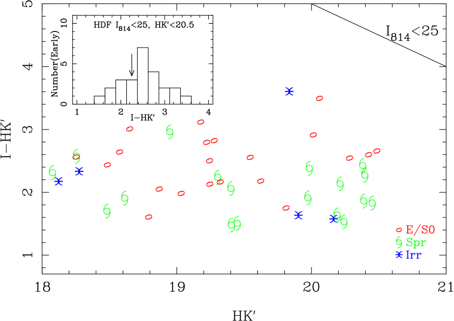
Figure 10: The colour-magnitude diagram of visually-classed objects within the deeper sample possible solely for the HDF ($I_{814}$ $<23$, $HK^{\prime}<$20.5). The inset histogram shows the $I_{814}-HK^{\prime}$ colour distribution for visually-classed spheroidal within the deeper sample. The arrow shows the peak of the distribution in the primary sample. Symbols are as for Figure 9

3.5 Alternative Star Formation Histories

The single burst models ruled out by the colours of speroidals in the previous sections are idealised representations of spheroidal history. We now consider alternative histories which could be more consistent with our various datasets.

At its most fundamental level, the deficit of red spheroidals at faint limits appears to eliminate models with very short epochs of star formation at high redshifts followed by long quiescent periods. In the context of modelling distant red radio galaxies, Peacock et al (1998) have shows that models with continuous star formation truncated at later times avoid the peak luminosities associated with initial bursts and can produce a significant bluing at redshifts where the red tail would otherwise be seen. In an important recent paper, Jimenez et al. (1998) argue that monolithic models have been rejected prematurely by some authors: only extreme scenarios with very short duration bursts (eg. $10^{7}$ Myr) of star-formation followed by absolute quiescence can be ruled out, while bursts with fairly low-levels of extended star-formation activity may still be compatible with the observed data. On the basis of a simple one-dimension chemo-dynamical model for the evolution of spheroids, these authors predict that the integrated star-formation history of early-type galaxies should resemble a quasi-monolithic collapse model. A concrete prediction of this model is that the bulk of the star-formation in high-$z$ spheroids is occuring near their cores, an effect that appears to have been seen (Abraham et al. 1999), and which may be responsible for the blue colours of some ellipticals in our sample.

Figure 11: The colour difference between a 1.0 Gyr single burst and the same model plus a short burst of star formation as a function of the redshift, $z=z_{burst}$, where the burst is added is show for a series of redshift of observation ($z_{0}=0.2,0.5,0.7,1.0,1.5\mbox{~{}and~{}}2.0$). The horizontal dashed line represent $\delta_{colour}=0.3$ and the shaded area shows the range in $z_{burst}$ where $\delta_{color}\geq 0.3$ for each $z_{o}$.

In the light of the above, it is therefore interesting to calculate the amount of recent star formation which must be added to a single burst model in order for the model to match the observed $I_{814}-HK^{\prime}$ colours. We seek to determine the timescales over which such a system is bluer than the passive evolution model by at least $\delta_{colour}=(I_{814}-HK^{\prime})_{model}-(I_{814}-HK^{\prime})_{obs}\simeq 0.3$ mag, i.e. consistent with the typical colour offset from the solar metallicity tracks shown in Figure 9. To model this we added a short burst of star-formation (of duration 0.1 Gyr, forming 15% of the stellar mass) occurring at $z=z_{burst}$ to an underlying solar metallicity monolithic collapse model at a given redshift using the population synthesis models of Bruzual & Charlot (1996). We then computed the redshift range over which the burst at $z_{burst}$ results in $\delta_{color}>0.3$ for a given redshift of observation, $z_{o}$.

The result of this exercise is shown in Figure 11 for several redshifts of observation $z_{0}$. The range in redshift space where a 15% burst produces a blueing $\delta_{colour}\geq 0.3$ is shown as the shaded area. (For example, a galaxy observed at redshift $z_{o}=1$ would be at least 0.3 mag bluer than the monolithic collapse models between points A and B in the figure. At $z_{o}=0.5$ a burst would have to occur at $0.5<z_{burst}<0.65$, while for $z_{o}=0.7$ it would have to occur in the range $z_{burst}\sim 0.7-0.9$. Since almost all points in Figure 9 lie blueward of the solar metallicity model tracks, and since galaxies in our sample lying in the redshift range $0<z<1$ have “memory” of bursts over $\delta z\sim 0.1-0.2$, it seems improbable that moderate intensity (ie. 15% mass) single burst events can explain the colour offsets shown in Figure 9. It seems more probable that the duty-cycle of star-formation is more extended, indicative of either a low level of roughly continuous star-formation underlying the old stellar populations, or perhaps of a succession of lower mass bursts.

The preceeding analysis indicates the extent to which a modest “polluting” star-forming population superposed on a dominant old stellar population reconciles our observations with traditional monolithic collapse scenarios. In contrast to this, it is interesting to consider what sort of hierarchical formation models may also be consistent with the present data. The rather mild density evolution in our sample is in sharp disagreement with the predicted factor of three decline in the abundance of spheroidals at $z\sim 1$, based on the present generation of “semi-analytical” models in high-density, matter-dominated cosmologies (eg. Kauffmann & Charlot 1998a). However, in a flat $\Lambda$-CDM model (with $\Omega_{M}=0.3$, $\Omega_{\Lambda}=0.7$) the decline in the abundance of spheroidals is only 30% at $z\sim 1$ (Kauffmann & Charlot 1998b), and may be consistent with the present observations. In the latter model the oft-quoted factor of three decline in the space density of ellipticals occurs at $z=2$ instead of $z=1$, so future work extending the present sample to higher redshifts may allow us to distinguish between “extended” monolithic collapse scenarios and $\Lambda$-CDM hierarchical models. However, more detailed modelling in this particular case, e.g. of the colours distribution, is beyond the scope of this paper. If star-formation in extended monolithic-collapse scenarios is centrally concentrated (as suggested by the simple one-dimensional models of Jimenez et al. 1998), the two scenarios may also be distinguishable at lower redshifts on the basis of resolved colour distributions (Menanteau et al. 1999, in preparation).

4 CONCLUSIONS

We have constructed a new catalogue of $\simeq$300 faint field spheroidal galaxies using HST images for morphology to a limit of $I_{814}$ =23 mag. Follow-up infrared photometry has enabled us to consider the optical-infrared colour distribution of an infrared magnitude limited sample. We have modelled expected colours using various star formation histories, metallicities and cosmologies. For a limited subset, spectroscopic redshift data is available and within the HDF it is possible to construct a deeper catalogue.

Our main results can be summarised as follows:

$\bullet$ There is little evidence for strong evolution in the space density of luminous field spheroidal systems out to $z\sim 1$. Within the uncertainties introduced by poorly constrained values for the local spheroidal luminosity function and by $\Omega_{M}$ and $\Omega_{\Lambda}$, our data is consistent with no evolution, or with modest evolution (at the level of $\sim 30\%$) in terms of a decline in the space density of spheroidals by $z\sim 1$.

$\bullet$ Although we detect little evidence for strong evolution in the space density of luminous spheroidals, we find a marked deficit in the number of red spheroidals compared to predictions where the bulk of star formation was completed prior to $z\simeq$3.

$\bullet$ Where redshift data is available it suggests that the duty cycle for star-formation in high-redshift spheroidals is indicative of a low level of extended star-formation underlying a passively evolving population, rather than of relic star-formation following from a massive burst episode.

$\bullet$ The apparently mild density evolution and blue colours of high-redshift spheroidals in the present sample are consistent with the predictions of “extended” monolithic collapse scenarios, in which the existing star-formation pollutes the colours of a dominant, underlying old stellar population. The data is not consistent with the predictions of semi-analytical hierarchical models in high-density, matter-dominated cosmologies. However, the observed weak density evolution may be consistent with the predictions of hierarchical $\Lambda$-CDM models (Kauffmann & Charlot 1998b).

Spectroscopic redshifts for a complete sub-sample of our catalogue will enable models for the star-formation history of high redshift spheroidals to be rigorously tested, eliminating some of the ambiguities present in the current analysis.

Table 1: The HST Sample

Field	$I_{814}$	$V_{606}$	$H$+$K^{\prime}$	FWHM	$\alpha$(J2000)	$\delta$(J2000)	Nz	NE/S0
0029+13	6300	3300	3900	0.6”	00:29:06.2	13:08:12.9	…	…
0144+2	4200	…	2340	0.8”	01:44:10.6	02:17:51.2	…	…
0939+41	4600	5400	3120	0.9”	09:39:33.3	41:32:47.9	…	…
1210+39	4899	3999	3120	0.6”	12:10:33.3	39:29:01.6	…	…
1404+43	8700	5800	3120	0.7”	14:04:29.3	43:19:15.2	…	…
East	5300	…	10985	0.8”	12:37:02.0	62:12:23.4	…	…
HDF	123600	109050	10530	0.8”	12:36:47.5	62:13:04.4	30	18
NEast	2500	…	10595	0.8”	12:37:03.7	62:15:13.0	…	…
NWeast	2500	…	10985	0.8”	12:36:49.4	62:15:53.8	…	…
OutEast	3000	…	10985	0.8”	12:37:16.2	62:11:42.5	…	…
OutWest	2500	…	10270	0.8”	12:36:19.3	62:14:25.5	…	…
SEast	2500	…	10465	0.8”	12:36:46.2	62:10:14.6	…	…
SWest	2500	…	10395	0.8”	12:36:32.0	62:10:55.3	…	…
West	5300	…	11375	0.8”	12:36:33.6	62:13:44.9	…	…
cfrs031	6700	…	3120	0.8”	03:02:57.4	00:06:04.9	8	4
cfrs033	6700	…	3120	0.7”	03:02:33.0	00:05:55.2	5	1
cfrs034	6400	…	3120	0.8”	03:02:49.8	00:13:09.2	5	1
cfrs035	6400	…	3120	1.0”	03:02:40.8	00:12:34.3	2	1
cfrs101	6700	…	3120	0.8”	10:00:23.2	25:12:45.1	7	2
cfrs102	6700	…	3120	0.7”	10:00:36.5	25:12:40.1	9	6
cfrs103	5302	…	3120	0.6”	10:00:46.7	25:12:26.3	12	7
u26x1	4400	2800	4420	0.8”	14:15:20.1	52:02:49.9	…	…
u26x2	4400	2800	3120	0.7”	14:15:13.7	52:01:39.6	…	…
u26x4	4400	…	3120	0.7”	14:18:03.2	52:32:10.4	…	…
u26x5	4400	…	3315	0.7”	14:17:56.7	52:31:00.6	…	…
u26x6	4400	…	3120	0.5”	14:17:50.3	52:29:50.8	…	…
u26x7	4400	…	3120	0.7”	14:17:36.9	52:27:31.2	…	…
u2ay0	25200	24399	4160	1.4”	14:17:42.7	52:28:31.3	…	…
u2iy	7400	…	3120	0.6”	14:17:43.1	52:30:23.3	…	…
u3d3	4200	3300	3120	1.3”	20:29:39.6	52:39:22.3	…	…
ubi1	6300	3300	2600	0.6”	01:10:00.7	-02:27:22.2	5	1
uci1	10800	4800	3900	0.4”	01:24:41.6	03:51:24.2	…	…
ueh0	12600	8700	3900	0.5”	00:53:24.1	12:34:01.9	4	2
uim0	11800	…	4090	0.6”	03:55:31.4	09:43:31.9	5	1
umd4	9600	2400	3900	0.7”	21:51:06.9	28:59:57.0	…	…
uop0	4200	7200	3120	0.9”	07:50:47.9	14:40:39.1	…	…
uqc01	7200	7800	3120	1.0”	18:07:07.3	45:44:33.5	…	…
usa0	6300	5400	3120	0.7”	17:12:24.0	33:35:51.2	…	…
usa1	6300	5400	3900	0.5”	17:12:24.7	33:36:03.0	…	…
usp0	4200	3300	3120	0.9”	08:54:16.9	20:03:35.5	…	…
ust0	23100	16500	3120	0.9”	10:05:45.8	-07:41:21.0	…	…
ut21	11999	3600	3900	0.8”	16:01:13.2	05:36:03.2	…	…
ux40	7500	3300	3900	0.6”	15:19:40.3	23:52:09.9	5	3
ux41	6000	3300	3120	0.8”	15:19:54.6	23:44:57.8	…	…
uy402	5400	1400	3120	0.8”	14:35:16.0	24:58:59.9	…	…
uzk0	8700	8400	3120	0.9”	12:11:12.3	39:27:04.8	…	…
uzp0	6300	3300	3120	0.8”	11:50:28.9	28:48:35.2	…	…
uzx05	4700	2600	3120	0.7”	12:30:52.7	12:18:52.5	…	…

Table 2: Log of Observations

Program Date	Fields Observed	$\langle$Seeing$\rangle$	Telescope
Feb 6-8 1996	HDF	1.0”	UH-2.2m
Apr 5-8 1996	HDF	1.0”	CFHT
Apr 17-22 1996	8 HDF-FF	0.8”	UH-2.2m
Aug 20-24 1997	21 MDS fields	0.8”	UH-2.2m
Jan 18-20 1998	23 MDS fields	0.8”	UH-2.2m
Feb 12-13 1998	11 MDS fileds	0.7”	UH-2.2m

Table 3: Absolute Numbers

Data Set	$N_{early}$	$N_{early}^{I_{814}-HK^{\prime}>3.0}$	Total Excessb	Red Fraction Excessc
Observational data (with bootstrapped errors)
Visually Classified	$266\pm 13$	$26\pm 5$
Visually Classified + Compacts	$316\pm 14$	$40\pm 5$
A/C classified	$323\pm 13$	$40\pm 6$
Pozzetti et al LFa ($\alpha=-0.48$)
40% Solar $\Omega_{M}=0.0$ $\Omega_{\Lambda}=0.0$	357.17	72.63	$1.34_{1.28}^{1.41}$	$2.79_{2.34}^{3.46}$
100% Solar $\Omega_{M}=0.0$ $\Omega_{\Lambda}=0.0$	366.57	135.26	$1.38_{1.31}^{1.45}$	$5.20_{4.36}^{6.44}$
250% Solar $\Omega_{M}=0.0$ $\Omega_{\Lambda}=0.0$	372.85	198.09	$1.40_{1.34}^{1.47}$	$7.62_{6.39}^{9.43}$
40% Solar $\Omega_{M}=0.3$ $\Omega_{\Lambda}=0.7$	433.94	90.37	$1.63_{1.56}^{1.72}$	$3.48_{2.92}^{4.30}$
100% Solar $\Omega_{M}=0.3$ $\Omega_{\Lambda}=0.7$	449.58	168.27	$1.69_{1.61}^{1.78}$	$6.47_{5.43}^{8.01}$
250% Solar $\Omega_{M}=0.3$ $\Omega_{\Lambda}=0.7$	458.74	247.12	$1.72_{1.64}^{1.81}$	$9.50_{7.97}^{11.77}$
Marzke et al LFa ($\alpha=-1.00$)
40% Solar $\Omega_{M}=0.0$ $\Omega_{\Lambda}=0.0$	240.29	28.56	$0.90_{0.86}^{0.95}$	$1.10_{0.92}^{1.36}$
100% Solar $\Omega_{M}=0.0$ $\Omega_{\Lambda}=0.0$	259.81	65.18	$0.98_{0.93}^{1.03}$	$2.51_{2.10}^{3.10}$
250% Solar $\Omega_{M}=0.0$ $\Omega_{\Lambda}=0.0$	286.76	113.26	$1.08_{1.03}^{1.13}$	$4.36_{3.65}^{5.39}$
40% Solar $\Omega_{M}=0.3$ $\Omega_{\Lambda}=0.7$	284.40	35.43	$1.07_{1.02}^{1.12}$	$1.36_{1.14}^{1.69}$
100% Solar $\Omega_{M}=0.3$ $\Omega_{\Lambda}=0.7$	311.23	80.37	$1.17_{1.12}^{1.23}$	$3.09_{2.59}^{3.83}$
250% Solar $\Omega_{M}=0.3$ $\Omega_{\Lambda}=0.7$	344.91	139.39	$1.30_{1.24}^{1.36}$	$5.36_{4.50}^{6.64}$

Appendix A Calculation of the Luminosity-weighted Mean Metallicity of a Spheroidal Galaxy Interior to an Isophotal Limit

Elliptical galaxies are known to contain highly enriched cores with strong metallicity gradients. Because of cosmological dimming, in the present paper we sample ellipticals at a range of rest-frame limiting isophotes, and it is important to have at least a qualitative understanding of the effects of metallicity gradients on the sampled starlight probed by our data. It is shown in Arimoto et al (1997) that the mean luminosity-weighted iron abundance of spheroidal systems with $R^{1/4}$ profiles integrated to infinity is similar to the abundance measured at the effective radius. It is straightforward to generalize the integral in equation (6) of Arimoto et al (1997) to calculate $\langle Z(R)\rangle$, the mean metallicity of an $R^{1/4}$ law spheroid within a given isophotal radius $R$, as a fraction of the metallicity measured within the effective radius, $R_{e}$. For a circularly symmetric galaxy the resulting expression is analytically tractable. The $R^{1/4}$ law giving surface brightness $I(R)$ as a function of radius $R$ is parameterized as follows:

$$I(R)=\exp\left\{-b\left[{\left(R\over R_{e}\right)}^{1/4}-1\right]\right\}$$ (1)

where $R_{e}$ is the half-light radius, and $b=3.33\ln(10)$. Metallicity gradients can be parameterized by a power-law index $c$ as a function of radius:

$$Z(R)=Z(0)\left({R\over R_{e}}^{-c}\right).$$ (2)

Essentially all of the ellipticals studied by Arimoto et al. (1997) have gradients parameterized by $0<c<1.3$, with metallicities of up to several hundred percent solar in their cores decreasing to roughly solar abundance at the effective radius.

Integrating equation (6) of Arimoto et al (1997) to a radius $R$ instead of to infinity yields the mean metallicity interior to a radius R, expressed in units of the mean metallicity interior to radius $R_{e}$:

$$\langle Z(R)\rangle=-e^{b(-1+R^{1/4})}{A/B}\\$$ (3)

where

$$A = [-5040b-2520b^{2}-840b^{3}-210b^{4}-42b^{5}$$ (5)

$$-7b^{6}-b^{7}+5040(-1+E^{b})]\cdot$$

$$[\Gamma(8-4c)-\Gamma(8-4c,bR^{1/4})]$$

$$B = [-5040(-1+e^{bR^{1/4}})+5040bR^{1/4}$$ (8)

$$+2520b^{2}\sqrt{R}+840b^{3}R^{3/4}+210b^{4}R+$$

$$42b^{5}R^{5/4}+7b^{6}R^{3/2}+b^{7}R^{7/4}]\cdot$$

$$[\Gamma(8-4c)-\Gamma(8-4c,b)].$$

(Note that in the preceeding expression, $\Gamma(x)$ is the Euler gamma function, and $\Gamma(x,y)$ is the incomplete gamma function).

Figure 12: The mean luminosity-weighted metallicity as a function of isophotal radius. Metallicity is given as a fraction of the metallicity interior to the half-light radius $R_{e}$. Radii are expressed in units of the half-light radius. The dotted line corresponds to $c=1.3$, and the solid line to $c=0.4$.

Mean metallicities as a function of radius are shown in Figure A1 for values of $c=0.4$ and $c=1.3$, spanning the range of metallicity gradients typically seen in luminous ellipticals. As expected, the luminosity-weighted metallicity as a function of isophotal radius rises sharply at $R\ll R_{e}$, but for our present purposes the important feature to note in Figure 12 is the shallow decline beyond $R>0.5R_{e}$ in the luminosity-weighted mean metallicity, regardless of the strength of the power-law slope $c$ parameterizing the metallicity gradients. This behaviour was also noted by Arimoto et al. 1997 in their simplified calculation. The overall metallicity of the galaxy can be well-characterized by the mean metallicity interior to the effective radius (ie. $\sim$ solar in the Arimoto et al. sample) over an extraordinarily large range in isophotal radius. We can thus make fair comparisons between ellipticals over a broad range of redshifts in spite of cosmological dimming of the rest-frame isophote, provided only the ellipticals are observed with sufficient signal-to-noise that their isophotal radii are at least as large as their effective radii. This is the case for the vast majority of ellipticals in the present sample — only at very high redshifts, where compact ellipticals have limiting isophotes comparable to their effective radii, is the mean luminosity-weighted metallicity expected to deviate from that at the effective radius.

References

- [] Abraham, R. G., Tanvir, N. R., Santiago, B. X., Ellis, R. S., Glazebrook, K. & van den Bergh, S. 1996a, MNRAS, 279, L47
- [Abraham et al. 1996b] Abraham, R. G., van den Bergh, S., Ellis, R. S., Glazebrook, K., Santiago, B. X., Griffiths, R. E., Surma, P. 1996b, ApjSS, 107, 1
- [] Abraham, R. G., Smecker-Hane, Tammy A., Hutchings, J. B., Carlberg, R. G., Yee, H. K. C., Ellingson, Erica, Morris, Simon, Oke, J. B., Rigler, Michael, 1996c, ApJ, 471, 694
- [] Abraham,R. G., Ellis,R. S., Fabian, A. C., Tanvir, N. R. and Glazebrook, K., 1998 MNRAS (astro-ph/9807140)
- [] Arimoto, N., Matsushita, K., Ishimaru, Y., Ohashi, T., & Renzini, A. 1997, ApJ, 477, 128
- [] Baade, W. 1957 in Stellar Populations, ed. O’Connell, D.J.K. p3, Vatican (Rome).
- [] Barger, A. J., Aragon-Salamanca, A., Ellis, R. S., Couch, W. J., Smail, I., Sharples, R. M.,1996, MNRAS, 27, 1
- [] Barger, A. J., Cowie, L. L., Trentham, N., Fulton, E., Hu, E. M., Songalia, A. & Hall, D., 1998, ApJ (in press)
- [] Baugh, C. Cole, S. & Frenk, C.S. 1996 MNRAS 283, 1361.
- [] Bertin, E. & Arnouts, S. 1996 Astron. Astrophys. Suppl. 117, 393.
- [] Bower, R.G., Lucey, J.R. & Ellis, R.S. 1992 MNRAS 254, 601.
- [] Brinchmann, J., Abraham, R.G., Schade, D. et al 1998 Ap J 499, 112.
- [] Broadhurst, T.J., Ellis, R.S. & Glazebrook, K. 1992 Nature
- [] Bruzual, G. & Charlot, S. 1993 Ap J 405, 538
- [] Bruzual, G. & Charlot, S. 1996, GISSEL (in preparation)
- [] Charlot, S. & Silk, J., 1994, ApJ, 432, 453
- [] Connolly, A.J., Szalay, A.S., Dickinson, M. SubbaRao, M.U. & Brunner, R.J. 1997 Ap J 486, 11
- [] Cowie, A.S., 1997 unpublished catalogue of HDF redshifts (see http://www.ifa.hawaii.edu/cowie/tts/tts.html)
- [] Driver, S.P., Windhorst, R.A., Ostrander, E.J., Keel, W.C. et al 1995 Ap J 449, L23.
- [] Dunlop, J. 1998 in The most distant radio galaxies, eds. Best, et al, Kluwer, in press (astro-ph/9801114)
- [] Efron, B. & Tibshirani, R. J. 1993. “An Introduction to the Bootstrap”, (Chapman & Hall:New York)
- [] Ellis, R.S. Smail, I., Dressler, A. et al 1997 Ap J 483, 582
- [] Glazebrook, K., Ellis, R.S., Santiago, B. & Griffiths, R.E. 1995 MNRAS 275, L19.
- [] Glazebrook, K., Abraham, R., Santiago, B., Ellis, R.S., & Griffiths, R. 1998 MNRAS 297, 885.
- [] Governato, F., Baugh, C.M., Frenk, C.S. et al 1998 Nature 392, 359
- [] Groth, E., Kristian, J.A., Lynds, R. et al 1994 Bull. AAS 185, 53.09
- [] Hogg, D.W., Cohen, J.G., Blandford, R. et al 1998 AJ 115, 1418
- [] Im, M & Casertano, S. 1998 preprint
- [] Im, M. Griffiths, R.E., Ratnatunga, K.U. & Sarajedini, V.L. 1996 Ap J 461, L9
- [] Jimenez, R., Friaca, A., Dunlop, J., Terlevich, R., Peacok, J. & Nolan, L. 1999 MN submitted (astro-ph 9812222)
- [] Kauffmann, G., Charlot, S. & White, S.D.M. 1996 MNRAS 283, L117.
- [] Kauffmann, G. & Charlot, S. 1998a MNRAS 297, L23.
- [] Kauffmann, G. & Charlot, S. 1998b, preprint (astro-ph/9810031).
- [] Lilly, S.J., Tresse, L., Hammer, F., Crampton, D. & LeFévre, O. 1995 Ap J 455, 108
- [] Lilly, S.J., LeFévre, O., Hammer, F. & Crampton, D. 1996 Ap J 460, L1.
- [] Marzke, R.O., da Costa, L.N., Pellegrini, P.S., Willmer, C.N.A. & Geller, M.J. 1998 Ap J in press (astro-ph/9805218)
- [] Menanteau, F., Abraham, R.G. & Ellis, R.S. 1999 (in preparation)
- [] Moustakas, L.A., Davis, M., Graham, J. & Silk, J. 1997, ApJ, 475, 445.
- [] Peacock, J.A., Jimenez, R., Dunlop, J., Waddington, I. et al 1998 MNRAS in press (astro-ph/9801184)
- [] Perlmutter, S. et al 1999 ApJ, in press (astro-ph/9812133)
- [] Pozzetti, L. Bruzual, G., Zamorani, G., 1996 MNRAS 281, 953
- [] Rose, J., Bower, R.G., Caldwell, N. et al 1994 AJ 108, 2054
- [] Sandage, A. 1986 in Deep Universe, ed. Binggeli, B. & Buser, R. p1, Springer-Verlag (Berlin).
- [] Sandage, A., Visvanathan, N. 1978 Ap J 223, 707
- [] Schade, D. Lilly, S.J., Crampton, D. et al 1998 in preparation
- [] Stanford, S.A., Eisenhardt, P.R. & Dickinson, M. 1998 Ap J 492, 461.
- [] Totani, T. & Yoshii, Y. 1998 preprint (astro-ph/9805262)
- [] van den Bergh, S., Abraham, R. G., Ellis, R. S., Tanvir, N. R., Santiago, B. X., Glazebrook, K. G.,1996, AJ, 112, 359
- [] van Dokkum, P., Franx, M., Kelson, D.D. et al 1998 Ap J, in press (astro-ph/9807242)
- [] Wang, Y., Bahcall, N. & Turner, E.L. 1998 AJ in press (astro-ph/ 9804195).
- [] Williams, R.E., Blacker, B., Dickinson, M. et al 1996 AJ 112, 1335.
- [] Windhorst, R., Driver, S.P., Ostrander, E.J. et al 1996 in Galaxies in the Young Universe, ed. Hipperlein, H., p265, Springer-Verlag (Berlin).
- [] Zepf, S.E. 1997, Nature, 390, 377