SCUBA - A submillimetre camera operating on the
James Clerk Maxwell Telescope

Abstract

The Submillimetre Common-User Bolometer Array (SCUBA) is one of a new generation of cameras designed to operate in the submillimetre waveband. The instrument has a wide wavelength range covering all the atmospheric transmission windows between 300 and 2000 $\mu{m}$. In the heart of the instrument are two arrays of bolometers optimised for the short (350/450 $\mu{m}$) and long (750/850 $\mu{m}$) wavelength ends of the submillimetre spectrum. The two arrays can be used simultaneously, giving a unique dual-wavelength capability, and have a 2.3 arc-minute field of view on the sky. Background-limited performance is achieved by cooling the arrays to below 100 mK. SCUBA has now been in active service for over a year, and has already made substantial breakthroughs in many areas of astronomy. In this paper we present an overview of the performance of SCUBA during the commissioning phase on the James Clerk Maxwell Telescope (JCMT).

Keywords: Submillimetre astronomy: JCMT, Bolometer arrays: SCUBA

1 INTRODUCTION

Until recently, the only instruments available for continuum astronomy in the submillimetre waveband were single-channel, broadband photometers[1]. Not only was mapping extended regions of sky painstakingly slow, but instrument sensitivity was invariably detector-noise limited at all wavelengths of operation. SCUBA is the most sensitive and versatile of a new breed of imaging devices now available for the submillimetre region[2, 3].

The instrument consists of two arrays of bolometers (or pixels); the Long Wave (LW) array has 37 pixels operating in the 750 and 850 $\mu{m}$ atmospheric transmission windows, while the Short Wavelength (SW) array has 91 pixels for observations at 350 and 450 $\mu{m}$. Each of the pixels has diffraction-limited resolution on the telescope, and are arranged in a closed-packed hexagon (as shown in Figure 1). Both arrays have approximately the same field-of-view on the sky (diameter of 2.3 arc-minutes), and can be used simultaneously by means of a dichroic beamsplitter. In addition, there are three pixels available for photometry in the transmission windows at 1.1, 1.35 and 2.0 mm, and these are located around the edge of the LW array.

SCUBA was a giant step forward on two major technical fronts: Firstly, it was designed to have a sensitivity limited by the photon noise from the sky and telescope background at all wavelengths, i.e. achieve background limited performance. This is achieved by cooling bolometric detectors to 100 mK using a dilution refrigerator, while limiting the background power by a combination of single-moded conical feedhorns and narrow-band filters. The second innovation came in the realisation of the first large-scale array for submillimetre astronomy (arbitrarily defined here as greater than 100 detectors in total!). This multiplex advantage means that SCUBA can acquire data thousands of times faster than the previous (single-pixel) instrument to the same noise level.

SCUBA was designed and constructed by the Royal Observatory in Edinburgh (ROE) in collaboration with Queen Mary and Westfield College. It was delivered to the Joint Astronomy Centre in April 1996, with first light on the telescope in July 1996. After a lengthy commissioning period, SCUBA began taking observations for the astronomical community in May 1997. In this paper we present an overview of both the instrument characterisation and the telescope performance from the commissioning phase. SCUBA is still evolving, with new and innovative ways to take data and remove the effects of the atmosphere being developed all the time. In the final section we briefly discuss potential ways of improving the performance in the next few years.

Figure 1: The pixel layout for the SCUBA Short-Wave and Long-Wave arrays. The locations of the photometric pixels (1.1, 1.35 and 2.0 mm) are also shown.

2 Instrument performance

2.1 Bolometer characterisation

The SCUBA bolometers are of a composite design, with an NTD germanium thermometer[4] bonded to a sapphire substrate. The incoming radiation is absorbed onto a thin film of bismuth mounted on the substrate. Electrical connections are made by 10 $\mu{m}$ diameter brass wire, which governs the overall thermal conductance, and these leads are fed out of the back of the mount. Each bolometer is designed as a $``$plug-in$"$ unit which can be close-packed to form an array, and easily replaced in event of malfunction. The cylindrical body design acts as an integrating cavity, which is fed by a single-moded circular waveguide from a conical feedhorn. Each bolometer is included in a bias circuit with individual 90 M$\Omega$ load resistor (also cooled to 100 mK) and common battery bias supply. Signals are taken from the bolometers to dc-coupled, cold JFET head amplifiers via woven niobium-titanium ribbon cables, and then out of the cryostat to room-temperature ac-coupled amplifiers through RF filters. The bolometer design and construction is discussed more fully in Holland et al.[5], and the signal processing chain by Cunningham et al[2].

2.1.1 V-I curves

A typical set of voltage-current (V-I) measurements for the central pixel of the LW array at 850 $\mu{m}$ are shown in Figure 2. These data were recorded for four background power levels: viewing ambient Eccosorb (293 K), a cold load (temperature about 45 K), liquid-nitrogen (77 K) and a filter blank at liquid helium temperatures (3.5 K). The background power loading on the detector is clearly seen to increase as a function of temperature. The cold load is effected by placing a mirror over the cryostat window, and produces a background power on the arrays of approximately 30 pW, very close to that expected from the sky under very good conditions at 850 $\mu{m}$ (see section 2.1.2). Since the filter bandwidths are almost identical at 450 and 850 $\mu{m}$ the amount of background power on each pixel, from a fixed temperature load at the window, is essentially the same, and this is clearly seen in the measured V-I curves at the two wavelengths.

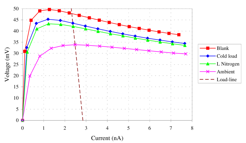
Figure 2: Voltage-current characteristics for a SCUBA bolometer at 850 $\mu{m}$, for four different backgrounds.

When optimally biased, as indicated by the load-line, the bolometers have an operating d.c. resistance of about 18 M$\Omega$ under the cold load background. The electrical responsivity is typically around 280 MV/W and has been found to vary by no more than $\pm$ 8% across the arrays. The figure shows that the V-I characteristics are significantly non-linear. For SCUBA bolometer material, electric-field induced non-linearity of the V-I has been seen to increase significantly as the operating temperature is reduced below 0.3 K. Two possible explanations for this are that the d.c. resistance has a strong electric field dependence, or that the electrons in the lattice become decoupled from the phonons at low temperatures resulting in a hot-electron effect. These possibilities are further discussed with reference to SCUBA data by Holland et al. (in prep).

2.1.2 Noise performance

A plot of the noise voltage versus frequency at optimum bias is given in Figure 3. In this plot the LN trace has been replaced by one in which the instrument views the zenith sky under excellent conditions at 850 $\mu{m}$ (precipitable water vapour level $<$ 1mm). The intrinsic detector noise (which can be assumed to that viewing the LHe blank) is clearly less than when viewing the sky, and this demonstrates that the detectors are background photon noise limited at this wavelength. During the normal operating modes of the instrument the bolometers are required to respond to frequencies in a 3–11 Hz signal band (for the scan-map observing mode). This band is free from any distinct features that may degrade the instrument sensitivity. There is also little $``$1/f” noise, except when the instrument views the zenith (this is low-frequency excess sky noise). Johnson noise dominates the intrinsic detector noise, and the noise level for each background level agrees very well with models based on the bolometer construction.

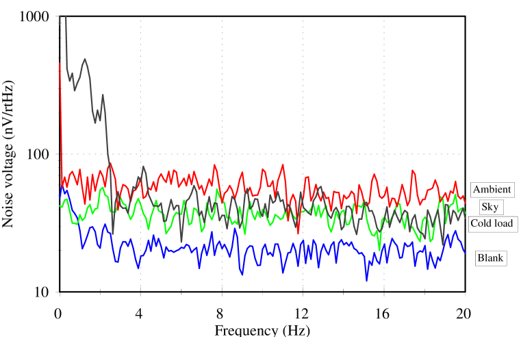
Figure 3: Noise spectra for a central pixel of the LW array at 850 $\mu{m}$ for four different background levels.

One crucial goal of the instrument is to achieve uniform noise performance over the entire array. Figure 4 shows how the demodulated chop-frequency (8 Hz) noise level varies for all array bolometers under the cold load background. In general, the noise stability is very uniform, with $\approx$ 10% of bolometers having a level $>$ 50 nV/Hz^1/2. The mean noise level across the arrays, discounting these bad pixels, is 40 $\pm$ 6 nV. For the pixels that do not meet the specification, the noise signature is predominantly 1/f noise and is believed to be due to poor contacts in the ribbon cables, and not intrinsic to the bolometers themselves. This beautifully illustrates the uniform behaviour obtainable with NTD germanium bolometers. In addition, throughout the laboratory testing phase there has only been one identified faulty bolometer (this corresponds to a yield of over 99%), and there has been no clear evidence for any deterioration in the overall noise performance.

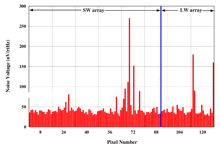
Figure 4: Variation in the demodulated chop-noise across the SCUBA arrays.

2.1.3 Optical responsivity

The optical responsivity was estimated from the power absorbed between two known temperature V-I curves. This gives an d.c. optical responsivity of approximately 250 MV/W at the cryostat window under background power levels of about 30 pW (cold load). Using the measured speed of response of the detectors (6 msec) the responsivity at a chop frequency of 8 Hz is 240 MV/W. The central pixel of the LW array has a performance slightly better than average across the arrays. The histogram in Figure 5 shows the spread in electrical and optical responsivity about mean levels of 270 MV/W (electrical) and 230 MV/W (optical). The spread in optical performance is greater than the electrical because of variations between the feedhorns. Again, this highlights the uniform performance across the 128 pixels within the SCUBA arrays.

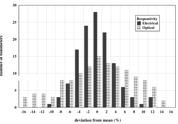
Figure 5: Electrical and optical responsivity variation across the SCUBA arrays.

2.1.4 Noise equivalent power (NEP)

Using the measured cold load noise voltage of 40 nV/Hz^1/2 and an optical responsivity of 230 MV/W, the measured optical NEP at the window of the cryostat is approximately 1.7 $\times$ 10^-16 W/Hz^1/2. Assuming that the zenith sky also has a noise level of about 40 nV (as shown in Figure 3), and at most a 7% loss in efficiency through the telescope optics and membrane, then the photon noise limited NEP on the sky is 1.8 $\times$ 10^-16 W/Hz^1/2. When blanked-off to incoming radiation the intrinsic NEP, determined from the V-I curve, is 6 $\times$ 10^-17 W/Hz^1/2. This clearly demonstrates that the performance is background limited, mainly from the sky, but also from contributions from the optics of the telescope and instrument.

2.2 Spectral coverage

Wavelength selection is determined by bandpass filters which are carefully designed to match the atmospheric transmission windows. The filters are multi-layer, metal-mesh interference filters and are located in nine-position rotating drum, surrounding the arrays. They have excellent transmission (typically over 80%), and have less than 0.1% out-of-band power leakage. The performance of the filters was originally measured at ambient temperature by a Fourier transform spectrometer (FTS) in the laboratory.

Late in 1996 the filter profiles were measured in-situ, and at the normal operating temperature (3.5 K) using the University of Lethbridge FTS[6]. All the array profiles were found to have shifted towards longer wavelengths, most into atmospheric lines of water vapour. This was the major reason why the initial sensitivities on the telescope were considerably worse than expected. Extensive testing at QMW in London showed that the shifting in wavelength was caused by a warping of the filter mounting rings when cold. New filters were manufactured using annealed stainless-steel rings, and after a modification to the way they were mounted in the drum, the re-measured profiles showed no appreciable shift in wavelength. The measured filter profiles are shown in Figure 6, together with the transmission curve for the atmosphere above Mauna Kea for 1mm of precipitable water vapour.

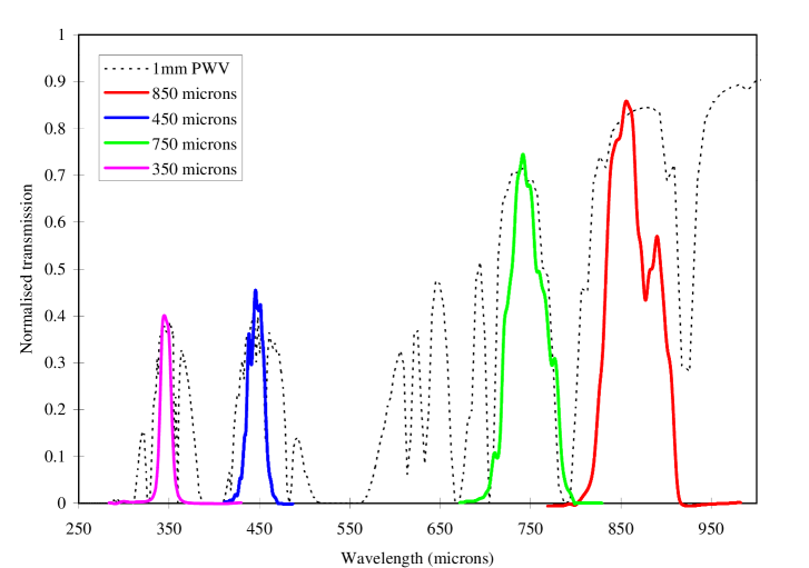
Figure 6: Measured filter profiles for the SCUBA array wavelengths, superimposed on the Mauna Kea atmospheric transmission curve for 1mm PWV. The 350 $\mu{m}$ filter was measured in the laboratory at a temperature of 77 K. Each profile has an arbitrary transmission axis, plotted to scale with the atmospheric windows.

2.3 Optical efficiency

The optical efficiency of the instrument (not including coupling to the telescope) can be estimated from the individual elements between the detector and the cryostat window. Assuming that the bolometer absorbs all incident power, and the feedhorns have negligible loss, then we expect an efficiency of 41 and 38% at 850 and 450 $\mu{m}$ respectively. The measured value, determined from the $\Delta$T V-I curves is only 24 and 21%, and so there is a loss of $\approx$ 70 % that can not be readily accounted for. This is further discussed in section 4.

3 Performance on the telescope

Figure 7 shows a side view of the SCUBA installed on the left-hand Nasmyth platform of the telescope. One consequence of the telescope having an altazimuth mount is that the field of view rotates during an observation. Since there is no mechanical field rotator this is compensated for in real-time software.

SEE ASSOCIATED JPEG IMAGE SCUBA2.JPG

Figure 7: Photograph of SCUBA on the left-hand Nasymth platform of the JCMT.

3.1 Observing modes

SCUBA is both a camera and a photometer. There are 4 basic observing modes available for use with SCUBA: photometry, jiggle-mapping, scan-mapping and polarimetry. These will be briefly described in the next section (a more extensive description of the first three is given by Lightfoot et al.[7]).

3.1.1 Photometry

Point-source photometry is carried out with the central pixel of each array simultaneously at two wavelengths, or with any of the photometric pixels independently. The conventional techniques of secondary mirror chopping and telescope nodding are adopted to remove the dominant sky background. Extensive tests have shown that better S/N is obtaining by performing a small 3 $\times$ 3 grid (of spacing 2 arc-seconds) around the source. This compensates for the slight offset between the two arrays (1.5 arc-seconds), and presumably helps cancel scintillation effects and/or slight pointing or tracking uncertainties.

3.1.2 Jiggle-mapping

Jiggle mapping is the adopted observing mode for sources that are smaller than the array field of view. Since the detectors are spaced in the focal plane by 2 $\times$ FWHM on the sky, the secondary mirror is jiggled to fill in the gaps, and produce a fully-sampled map. It requires 16 jiggles to fully-sample a source at one wavelength. When using both arrays simultaneously (the default) a 64-point jiggle pattern is required. Such a map is normally split into 4 sections, and after each section the telescope is nodded to the other beam. Limited mosaicing of jiggle-maps is also possible.

3.1.3 Scan mapping

Scan mapping is used to map regions that are extended compared with the array field-of-view. This is an extension of the raster technique used with single-element photometers, where the telescope is scanned across a region whilst chopping to produce a differential map of the source. The SCUBA arrays have to be scanned at one of 6 angles (between 0 and 180 degrees) to produce a fully-sampled map. Data is acquired using a method first described by Emerson[8], where maps are taken at several different chop throws and directions. This significantly reduces the $``$restoration noise” of the traditional EKH technique[9], and results in substantial improvements in S/N. This new method is more fully discussed by Jenness et al.[10] in this volume.

3.1.4 Polarimetry

This is a very new observing mode for SCUBA, and requires additional hardware in the form of a photolithographic analyser to select one plane of polarisation and a rotating achromatic half-waveplate. Photometry is carried out a number of waveplate positions, and the amplitude and phase of the resulting sinusoidal modulation of the signal is used to deduce the degree of linear polarisation and position angle. At time of writing this observing mode has been commissioned in $``$single-pixel$"$ mode, with the prospects of full-imaging polarimetry by the end of 1998.

3.2 Sensitivity

The overall sensitivity on the telescope is represented by the noise equivalent flux density (NEFD), and is the flux density which produces a signal-to-noise of unity in a second of integration. The NEFD, particularly at the shorter wavelengths, depends very much on the weather, and on many occasions the fundamental limit to sensitivity is governed by $``$sky noise”. This is caused by spatial and temporal variations in the emissivity of the atmosphere passing over the telescope on short timescales. Our investigations of sky noise and its removal from SCUBA data are discussed by Jenness et al[10]. Table 1 summarises the per-pixel measured NEFD at all wavelengths, after sky noise removal, under the $``$best$"$ and $``$average$"$ conditions at each wavelength. These represent an order of magnitude improvement over the previous instrument at JCMT. In Table 2 we present 5-$\sigma$ detection limits based on the best NEFDs for 1, 10 and 25 hours on-source integration times.

Table 1: Measured NEFDs under best and average weather conditions on Mauna Kea.

Wavelength	Best NEFD	Average NEFD
($\mu$m)	(mJy/$\sqrt{Hz}$)	(mJy/Hz1/2)
350	1000	1600
450	450	700
750	110	140
850	75	90
1100	90	100
1350	60	60
2000	120	120

Table 2: 5-$\sigma$ detection limits for 1, 10 and 25 hours of integration time for the best SCUBA NEFDs.

Wavelength	NEFD	1-hr	10-hrs	25-hrs
($\mu$m)	(mJy/Hz1/2)	(mJy)	(mJy)	(mJy)
350	1000	83	26	17
450	450	38	12	7.5
850	75	6.3	2.0	1.3
1350	60	5.0	1.6	1.0

Since the instrument is predominantly background limited from the sky, the NEFD will vary with sky transmission, particularly at the submillimetre wavelengths. This variation can be calculated from,

$$NEFD=\frac{NEP_{ph}}{0.4\ A_{e}\ \eta\ e^{-\tau A}\ \Delta\nu}$$ (1)

where $NEP_{ph}$ is the photon noise limited NEP, $A_{e}$ the effective area of the telescope primary (102 m² at 850 $\mu{m}$ assuming a coupling efficiency of 70% to a point-source, and an rms surface accuracy of 30 $\mu{m}$), $\eta$ the optical efficiency (measured as 0.22 including telescope losses), $\tau$ the zenith optical depth (0.15 is close to the best achievable at 850 $\mu{m}$, $A$ the airmass of the source, and $\Delta\nu$ the radiation passband (30 GHz). The factor of 0.4 is included as an efficiency factor for chopping. Given a knowledge of the above parameters it is possible to construct a model of how the NEFD varies as a function of sky transmission. Figure 8 shows how the calculated NEFDs at 450 and 850 $\mu{m}$ vary with sky transmission. Also on this plot are some measured values from long ($\geq$ 15 minutes) photometry observations. As can be seen there is excellent agreement between the model and the measured points.

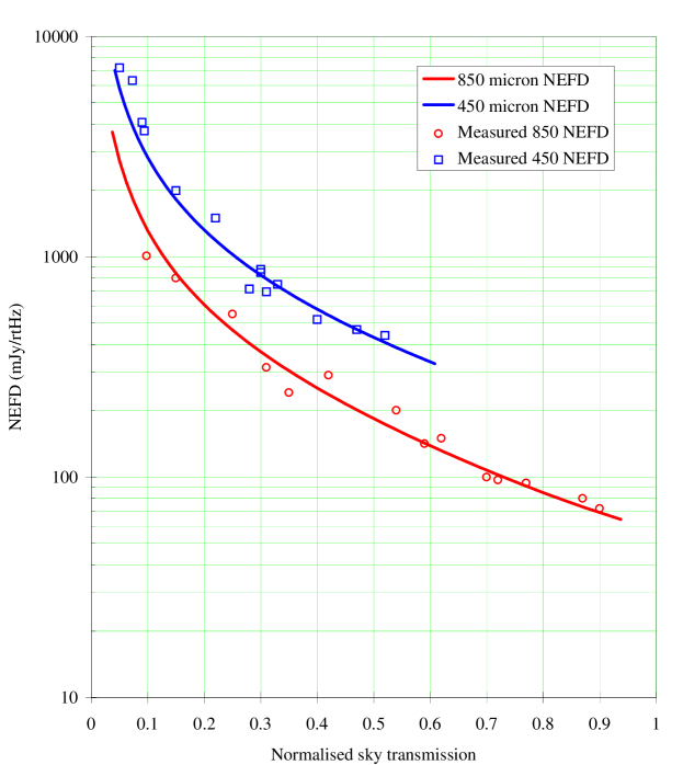
Figure 8: Model variation of the NEFD with sky transmission. Measured points are also shown by the symbols.

One of the primary scientific goals for SCUBA is to make deep integrations of faint sources, over a period of many hours, and so it is crucial that the noise integrates down in a predictable way. Figure 9 shows data coadded over a period of almost 5 hours, in which the standard error (solid line) integrates down with time as 95 (t/s)^-1/2.

Figure 9: Standard error evolution with time for a 5 hour photometry observation at 850 $\mu{m}$.

3.3 Optical performance

To obtain the maximum possible field of view at the Nasmyth focus, the normal f/12 focal ratio is extended to f/16 by a shift in the secondary mirror position. The resulting spherical aberration is removed by a corrector plate at the cryostat window. To minimise the thermal load on the low temperature stage, and the size of the feedhorns in the focal plane, the final focal ratio is down-converted to f/4. More details of the optical design are given in Murphy et al. (in prep).

The SCUBA optical system is almost entirely an all-mirror design (the exception being the corrector plate), and includes several off-axis mirrors to fold the telescope beam into a reasonably compact volume. Even though complex mirror shapes minimise aberrations to a large extent, some field curvature in the focal plane is inevitable. In addition, the bolometers have a range of optical responsivities, as indicated in Figure 5. Hence, the positions and relative responsivities of the bolometers must be accurately known for image resampling to work properly. The arrays are therefore flatfielded by scan-mapping the telescope beam over a bright point-like source (eg. Mars or Uranus). The flatfield has been found to remain extremely constant over the past year.

Diffraction-limited performance is illustrated at 450 and 850 $\mu{m}$ in Figure 10. These maps are centered on each array and are a 12 minute jiggle map of Uranus, chopping 60 arc-seconds in azimuth (E-W in the figure). The contours start at 2% and 1% of the peak at 450 and 850 $\mu{m}$ and then increase in the same steps. The measured full-width half maximum (FWHM) beam sizes are 7.8 and 13.8 arc-seconds at 450 and 850 $\mu{m}$ respectively.

One novel feature of the SCUBA optical design is an internal calibration system to take out long and short term drifts in the detector response. The internal calibrator (an $``$ inverse bolometer$"$) can be used to correct for variations in the sky background, or, if necessary, drifts in the base temperature of the refrigerator.

3.4 Vibrational microphonics

One of the early problems encountered with SCUBA on the telescope was unexpected high vibration levels from the secondary mirror unit. This affected about 10% of pixels, in addition to those suffering from 1/f noise. Of particular concern was the dominant 5th harmonic of the chop at around 40 Hz, which was interfering with the demodulation of the fundamental and internal calibrator signals. Increasing the rise-time of the chopper waveform by about 2 msec has improved the situation quite dramatically, without a noticeable loss in on-source efficiency (and consequently NEFD). Although one or two pixels remain slightly sensitive to vibration, particularly for large chop throws, this is no longer a major concern.

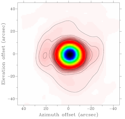
(a) (b)

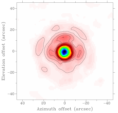
Figure 10: Beam maps of Uranus for the two array central pixels at (a) 850 $\mu{m}$ (10 contours starting at 1% of peak for the base, 1% intervals) and (b) 450 $\mu{m}$ (2% base, 2% intervals).

4 Future upgrades

It is possible that there is still a factor of 2 to be gained in NEFD at most wavelengths. One obvious way to improve the short wavelength performance in particular, is by improving the large scale surface accuracy of the telescope dish, and there is a programme already underway to accomplish this. For SCUBA itself there are several areas in which gains could be made, and these are briefly discussed in this section.

4.1 Improvements in sensitivity

4.1.1 Optical efficiency

In section 2.4 it was noted that the estimated and measured optical efficiencies differ by about 70% at 850 $\mu{m}$. Similar, or even larger discrepancies, exist at the other wavelengths. A small fraction of this loss could be accounted for in the bolometer absorption efficiency (for example, if the impedance match to free space is not optimum). The cause of the remaining loss is thought to be due to a subtle interaction between the array feedhorns and the filters. To make the inner system compact, and the filter diameters as small as possible, the arrays are in very close proximity to the filters in the drum. It is possible that a large array of feedhorns so close to the filters could modify the effective terminating impedance of the filters, resulting in a change to their reflectance coefficients. The net result could be that the horn beams leaving filter drum enclosure are considerably broader than when measured individually. If the beams are so wide that they over-illuminate the internal mirrors, then not only will the signal coupling to the telescope be reduced, but also additional photon noise will be introduced from the 45 K optics box.

One way of counteracting the rise in photon noise, if the horn beams themselves cannot be corrected, would be to terminate the spillover on a colder surface. An additional radiation shield at a temperature of $<$ 10 K would be complex and difficult to manufacture, but is nevertheless being considered.

4.1.2 Bolometer cavity tuning

FTS measurements were also carried out on the photometric pixels. The results showed a deep fringe roughly in the centre of the observed profile, and this fringe depth was seen to increase with wavelength. The reason for this is thought to be that the bolometer cavities do not scale with wavelength (i.e. they are all the same size). At the shorter (array) wavelengths the cavity behaves like a true integrating cavity, in which many modes propagate, and because radiation is coupled to the cavity at all wavelengths over the passband, absorption becomes more efficient. At the longer wavelengths fewer modes propagate in the cavity, thus losing the integrating properties.

A simple $``$tuning^′′ of the cavity at 1350 $\mu{m}$ (moving the waveguide exit closer to the substrate) gave an immediate factor of 2 improvement in NEFD (as shown in Table 1). Such gains are also expected at 1.1 and 2 mm in the near future. It is also possible that the photometric pixel bolometers could be re-designed to have a more optimum cavity design. It is unlikely, based on tests so far, that significant gains will be achievable at the array wavelengths by simply moving the position of the waveguide.

4.2 Improvements in noise performance

As mentioned in section 2.1.2 there are still some 10% of pixels that do not meet the noise specification. The reason for this is likely to be the copper-plated joints to the Nb-Ti ribbon cables. Fortunately, there has not been a deterioration in noise performance (eg. due to oxidisation or moisture when the instrument is opened). A new ribbon cable technology, being developed by ROE, should eliminate this problem.

4.3 Observing modes

Recent work has concentrated on improving the efficiency of all observing modes. In particular, the new scan-map observing mode, described by Jenness et al.[10], has demonstrated large improvements in achievable S/N (factors of 2–3) for mapping large areas of sky. More refinements to this mode are likely in the near future. For point-source photometry, chopping between bolometer positions is an obvious way to improve efficiency, and this is undergoing tests at the present time.

Another potential and very exciting observing technique is to utilise the versatility of the secondary mirror controller and the SCUBA data acquisition system (and transputer array) to record data very quickly. Full speed data on all SCUBA pixels can be taken with rates of 128 Hz or even higher. The previous functions of chopping and jiggling can be combined into a single stepping pattern, and in so doing should result in big savings in integration time (currently the telescope spends half of its time integrating on blank sky). Fully-sampled maps will also be obtained more quickly than the current technique, thereby rendering changes in atmospheric transmission less of a concern. More details of this are given by Le Poole et al. in this volume[11].

Array polarimetry is also an area that is being developed. Polarimetric data, from either dust continuum or synchrotron emission, can be used to deduce the magnetic field structure in a wide range of sources. Achromatic waveplates have been developed to allow simultaneous imaging using both arrays. Analysing the array polarisation data, correcting for instrumental polarisation contributions and sky rotation, is currently under investigation.

5 Scientific impact

After only a year in routine operation SCUBA has made a big impact on almost all areas of astronomy. Some of the areas that have benefited from SCUBA’s unprecedented sensitivity and mapping abilities are shown below.

• First real submillimetre images of a comet

• Light-curves of asteroids (and Pluto!)

• Searches for embedded protostars and pre-stellar cores

• Dust distribution around proto-planetary systems

• Study of detached shells in late-type stars

• Mapping the dust extent in nearby galaxies

• Starburst galaxy studies

• Imaging of massive nearby radio galaxies

• High red-shift galaxy surveys

• Lensing by galaxy clusters

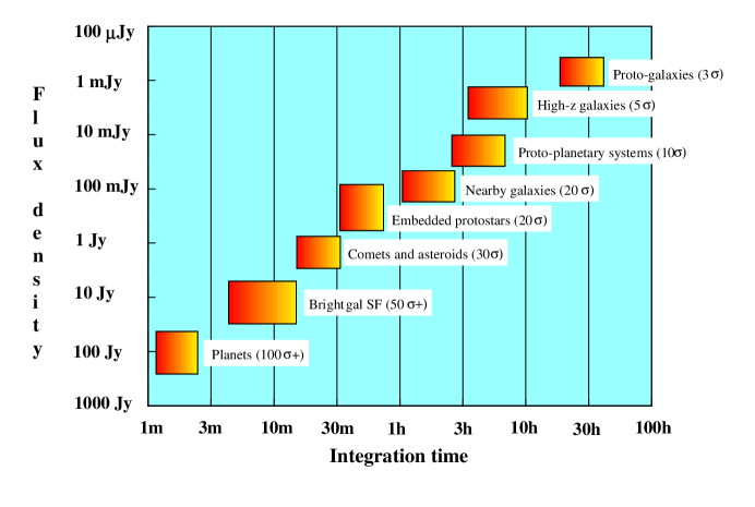
Figure 11: Typical SCUBA observational limits at 850 $\mu{m}$ for a wide range of astronomical sources.

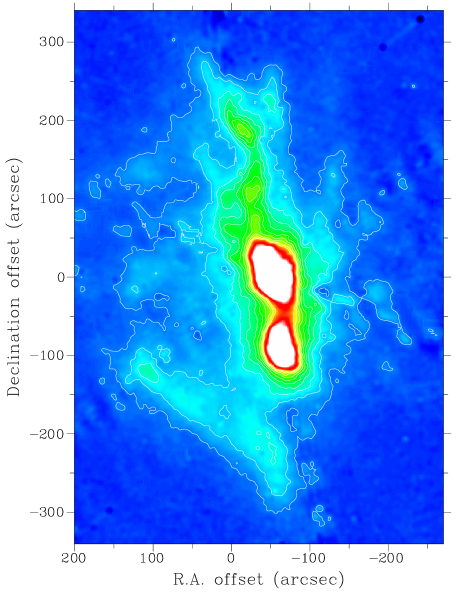
Figure 12: Scan-map of the central core of OMC1 at 850 $\mu{m}$. Contours start at 1% of the peak of OMC1 (150 Jy) and increment in 1% steps.

Figure 11 shows typical observational limits at 850 $\mu{m}$ for a wide variety of sources. These are based on programmes undertaken over the past year and illustrate the kind of limits that can be achieved. As an example of the mapping capabilities, Figure 12 shows an 850 $\mu{m}$ scan-map of the central bright core of the Orion Molecular Cloud. This 8 $\times$ 8 arc-minute map was obtained in just 50 minutes of integration time, and has a rms noise level of 60 mJy/beam. The Orion $``$bright-bar” is also clearly seen in this image, as well as the little-studied embedded protostellar ridge in the north.

6 Conclusions

SCUBA has proven to be an extremely powerful and versatile camera for submillimetre astronomy. Background photon noise limited performance on the telescope has been achieved by cooling the detectors to 100 mK and careful design of the focal plane optics. With an order of magnitude improvement in per-pixel sensitivity over the previous (single-pixel) instrument, and over 100 detectors in two arrays, SCUBA can acquire data approaching 10,000 times faster than was possible previously. It is clear that with this huge increase in performance, SCUBA will revolutionise submillimetre astronomy for many years to come.

References

- [1] W. D. Duncan, E. I. Robson, P. A. R. Ade, M. J. Griffin, and G. Sandell, “A millimetre/submillimetre common user photometer for the James Clerk Maxwell Telescope,” Mon. Not. R. Astron. Soc. 243, pp. 126–132, 1990.
- [2] C. R. Cunningham, W. K. Gear, W. D. Duncan, P. R. Hastings, and W. S. Holland, “SCUBA: the submillimeter common-user bolometer array for the James Clerk Maxwell Telescope,” Proc. SPIE 2198, pp. 638–649, 1994.
- [3] W. K. Gear and C. R. Cunningham, “SCUBA: A camera for the James Clerk Maxwell Telescope,” in Multi-feed systems for radio telescopes, D. T. Emerson and J. M. Payne, eds., ASP Conference Series 75, pp. 215–221, 1995.
- [4] E. E. Haller, “Physics and design of advanced ir bolometers and photoconductors,” IR Phys. 25, pp. 257–266, 1985.
- [5] W. S. Holland, P. A. R. Ade, M. J. Griffin, I. D. Hepburn, D. G. Vickers, C. R. Cunningham, P. R. Hastings, W. K. Gear, W. D. Duncan, T. E. C. Baillie, E. E. Haller, and J. W. Beeman, “100 mk bolometers for the Submillimetre Common-User Bolometer Array (SCUBA) i. Design and construction,” Int. J. IR&mm waves 17, pp. 669–692, 1996.
- [6] D. A. Naylor, T. A. Clark, and G. Davis, “A polarising Fourier transform spectrometer for astronomical spectroscopy at submillimeter and mid-infrared wavelengths,” Proc. SPIE 2198, pp. 529–538, 1994.
- [7] J. F. Lightfoot, W. D. Duncan, W. K. Gear, B. D. Kelly, and I. A. Smith, “Observing strategies for SCUBA,” in Multi-feed systems for radio telescopes, D. T. Emerson and J. M. Payne, eds., ASP Conference Series 75, pp. 327–334, 1995.
- [8] D. T. Emerson, “Approaches to multi-beam data analysis,” in Multi-feed systems for radio telescopes, D. T. Emerson and J. M. Payne, eds., ASP Conference Series 75, pp. 309–317, 1995.
- [9] D. T. Emerson, U. Klein, and C. G. T. Haslam, “A multiple beam technique for overcoming atmospheric limitations to single-dish observations of extended radio sources,” Astron. Astrophys. 76, pp. 92–105, 1979.
- [10] T. Jenness, J. F. Lightfoot, and W. S. Holland, “Removing sky contributions from SCUBA data,” Proc. SPIE 3357, 1998 (astro-ph/9809120).
- [11] R. Le Poole and H. W. van Someren Greve, “DREAM, the Dutch REal-time Acquisition Mode for SCUBA,” Proc. SPIE 3357, 1998.