Removing sky contributions from SCUBA data

Abstract

The Submillimetre Common-User Bolometer Array (SCUBA) is a new continuum camera operating on the James Clerk Maxwell Telescope (JCMT) on Mauna Kea, Hawaii. It consists of two arrays of bolometric detectors; a 91 pixel 350/450 micron array and a 37 pixel 750/850 micron array. Both arrays can be used simultaneously and have a field-of-view of approximately 2.4 arcminutes in diameter on the sky.

Ideally, performance should be limited solely by the photon noise from the sky background at all wavelengths of operation. However, observations at submillimetre wavelengths are hampered by “sky-noise” which is caused by spatial and temporal fluctuations in the emissivity of the atmosphere above the telescope. These variations occur in atmospheric cells that are larger than the array diameter, and so it is expected that the resultant noise will be correlated across the array and, possibly, at different wavelengths.

In this paper we describe our initial investigations into the presence of sky-noise for all the SCUBA observing modes, and explain our current technique for removing it from the data.

Keywords: Submillimetre astronomy, Bolometer arrays, SCUBA, sky-noise

1 INTRODUCTION

Observations at submillimetre wavelengths have always been severely hindered by the atmosphere, which is only partially transparent throughout the region. In addition to attenuating the signal, the atmosphere and the immediate surroundings of the telescope and the observatory contribute thermal radiation which is often a few orders of magnitude greater than the signal from the source under investigation. The necessity to extract the source signal from this background has led to the techniques of sky chopping and telescope nodding.

The aim of SCUBA is to be background limited, i.e. limited by the photon noise from the sky background. The main limit to sensitivity, particularly at the shorter submillimetre wavelengths arises from sky-noise. Sky-noise manifests itself in three ways: a D.C. offset, noise due to sky variability and scintillation. For this to be achieved the DC offset and effects of sky variability and scintillation must be removed. Chopping and nodding remove the DC offset and, in addition, diminish the effect of sky variability but don’t remove it completely.

Fig. 1 shows the noise spectrum for the centre pixel of the long-wave (LW) array at 850 microns. The bottom trace illustrates the system noise (i.e. the intrinsic detector and amplifier noise). The top trace shows the corresponding spectrum when the detector views the zenith sky under good observing conditions at 850 microns (approximately 1 mm of precipitable water vapour) with the chopper stationary. It can be seen that there is a “1/f” component to the zenith sky trace, extending out to 4 Hz or so, which is well above the system noise level.

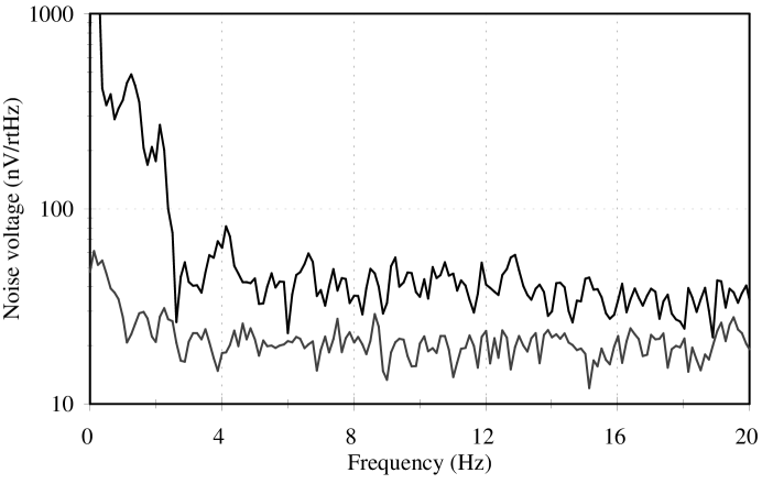
Figure 1: This figure shows noise spectra for a single pixel at 850 microns with no chopping (upper line) along with the system noise (lower trace). Clearly excess noise is visible below 3 Hz when looking at the sky.

Duncan et al.[1] have shown that two-position chopping at a frequency of approximately 8 Hz greatly reduces the sky-noise contamination in the power spectrum, but that on many occasions there is still a level of noise well above the system noise level.

There are several ways to reduce the residual sky-noise; firstly careful design of the filters to select the most transparent parts of the atmospheric window. Secondly, the chop throw should be kept as small as possible since the magnitude of sky-noise increases approximately linearly with chop throw amplitude[1]. Three-position chopping has also been found to produce considerable improvements. In this paper we concentrate our discussion on how to remove the error due to sky variability from array data taken with the Submillimetre Common-User Bolometer Array (SCUBA)[2, 3, 4] at the James Clerk Maxwell Telescope (JCMT).

2 Observing Modes with SCUBA

Three different observing modes are available[5]: two imaging modes (one for sources smaller than the array (jiggle mapping) and one for sources larger than the array (scan mapping)) and a photometry mode for measuring the flux density of point sources. The jiggle mapping and photometry modes have much in common and can be grouped together as ‘jiggle modes’ (a photometry observation is simply an under-sampled jiggle map). All these modes suffer from sky variability to a varying degree and each mode will be investigated in turn.

2.1 Jiggle modes

Both photometry and jiggle maps share the same basic observing method. The secondary mirror is chopped between the source position and sky at approximately 8 Hz to remove the bulk of the sky emission from the signal. SCUBA takes data at 128 Hz but currently hardware restriction mean that samples have a fixed integration time of 1 second. In order to remove slowly varying background emission and telescope asymmetries the telescope is nodded so that the source appears in the opposite beam. The nods are then subtracted before further processing so that each data point is in fact the difference between two 1 second integrations taken at different times – the time difference is directly related to the number of samples taken between each nod. It should also be noted that this technique results in pseudo-three beam data so that it is assumed that there is no source emission at any of the off-positions.

2.1.1 Photometry

The photometry mode is used to measure the flux density of point sources. In general a bolometer is centred on the source and a small jiggle pattern is used to compensate for any offsets between the two arrays: the standard jiggle pattern is a 3 by 3 grid with 2 arcsec spacing. For this configuration it takes $2\times 9$ seconds to complete an integration (nine seconds per nod) plus some overhead for moving the telescope. One important point is that data are taken for all bolometers even though only one is on source at any given time.

2.1.2 Mapping sources smaller than the array

As shown in Fig. 2a the individual bolometers are arranged in a hexagonal pattern to maximize packing efficiency. The size of the feedhorns means that the bolometers are separated by approximately 2 beam-widths so a fully-sampled image can not be taken in one go. To overcome this problem the secondary mirror is ‘jiggled’ to fill in the gaps so that a fully-sampled image can be obtained. For a single array 16 different secondary mirror positions are required for this but 64 positions are required when both arrays are being used simultaneously because of the factor of 2 difference in bolometer spacing between the arrays (see Fig. 2b).

(a) (b)

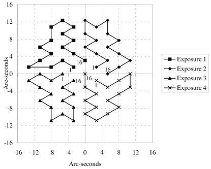
Figure 2: (a) The jiggle pattern used to fully-sample the long-wave array. The six nearest bolometers are shown to indicate the hexagonal packing of the array. (b) The jiggle pattern used to fully sample both array. Note that it is split into four sections so that the telescope can nod four times during an integration.

2.2 Mapping sources larger than the array

Jiggle mapping is not useable when there is a possibility of source emission in the off-beam. In this case a raster mapping technique is used where the telescope scans across the desired area whilst chopping.

3 Investigation of sky variability

This section will describe the differing ways in which sky variability manifests itself and the ways it can be removed.

We can only hope to remove sky variability if the size of the sky features are much larger than the array. The scale height of the ‘screen’ layer in the atmosphere that is moving over the telescope and causing the sky variation is of order 2 km or less. Combining this with typical wind speeds and the observed frequency of the fluctuations implies that the scale size of the fluctuations is of order 1000 arcsec or more so the error caused on something the size of the array should be well approximated by a DC offset.

3.1 Jiggle modes

The choice of chop configuration is critical for minimising the observed sky variability. In most cases azimuth chopping and nodding is used since this has been shown to be the best configuration for reducing systematics[6] but occasionally different chop directions are required (e.g. a chop in RA/dec to a fixed position on the sky or chopping between two bolometers on the array). The other important factor is the size of the chop throw – as the chop throw increases the sky cancellation becomes worse and the beam shape becomes more distorted.

3.1.1 Sky removal technique

The standard data reduction technique for jiggle data is:

1. The first stage in the data reduction process is to subtract the nods. This means that each processed data point is the difference of two one second samples taken 9 or 16 seconds apart.

2. Correct for atmospheric extinction and flatfield the data.

3. Identify sky bolometers or sky regions. For extended sources it is preferable to specify a sky region for all but the shortest observations. SCUBA is mounted on the nasmyth platform of an alt-az telescope with no image rotator such that during a long observation bolometers would see sky and source.

4. For each 2 second sample (2 seconds because of the nodding) calculate the average sky signal and subtract this from the entire array.

Currently no attempt has been made to remove a sky plane from the data. Preliminary investigations have been made but in general the effect has been small relative to the large scale DC offset.

3.1.2 Photometry

For most photometry observations the sources are known to be isolated and point-like and the chop throw can therefore be chosen to minimise systematics: two position chopping and nodding in azimuth are used[6] with small chop throws (30 to 60 arcsec).

Fig. 3 shows an example of some 850-micron photometry data with a sky transmission of approximately 80 per cent and seeing of 1.25 arcsec. For these data the measured sky variability contribution is approximately 0.12 mV (or approximately 30 mJy/beam) and when removed boosts the signal-to-noise by a factor of 2.

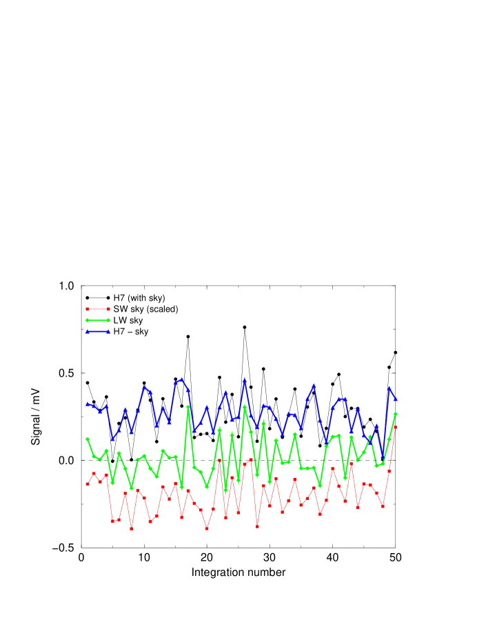
Figure 3: Sky and source signal for a 50 integration photometry observation at 850-microns. The lower trace shows the sky signal for the short-wave array (reduced by a factor of 5). In this case sky removal improves the signal-to-noise by a factor of 2.

All of the long integration photometry data taken between 1997 October and 1998 February have been processed in order to investigate sky variability for a set of different observations. It was expected that sky variability would increase during the daylight hours but, as shown in Fig. 4, these data do not show a large increase in sky variability during the morning. Although the number of data points taken before midnight are small there is a suggestion that the sky variability is higher for the first part of the night. Whilst these results seem to contradict the data presented later on for 64 position jiggle maps it must be remembered that photometry observations have much shorter integration times, chop throws and nod cycles. Additionally it is also possible that the months chosen are special in some way and more data analysis is required.

Figure 4: Magnitude of the measured sky variability plotted against the time of day.

Fig. 5 shows data for 250 observations with a linear least squares fit. Although the correlation is not perfect this preliminary result indicates that the magnitude of the sky variability seen on the short-wave array is proportional to that seen on the long-wave array.

Figure 5: Sky variability at 450 microns plotted against the sky variability for the short wave array for long photometry observations. A linear least squares fit is shown: the gradient is approximately 5.0 with a correlation coefficient of more than 0.9.

3.1.3 Mapping

Jiggle mapping suffers in two ways when compared with photometry mode:

1. The array has a diameter of more than two arcminutes, so it is necessary to chop at least this distance to avoid chopping onto the array.

2. The size of the jiggle pattern dictates that nodding will take place every 16 seconds. Whilst taking data on both arrays the jiggle pattern consists of 64 points, but a nod every 64 seconds is far too long even in the most stable conditions. For this case the pattern is split into 4 chunks of 16 so that nodding occurs every 16 seconds as for a single array observation (see Fig. 2b).

Fig. 6 shows a particularly good example of extreme sky variability with Fig. 6a showing the image before sky removal and Fig. 6b the image after sky removal. The time sequence for this observation is shown in Fig. 6c: the short-wave and long-wave sky are clearly correlated with variations in the central pixel. The upper trace of Fig. 6 shows the central pixel after sky removal and the signal variation repeats for each integration reflecting the fact that a 64 point jiggle pattern jiggles on and off the source.

These data were taken mid-morning and the lower trace of Fig. 6c shows that the large scale variations occur every 16 seconds reflecting the time taken for individual nods. Clearly, conditions were so unstable that a shorter nod period was desirable although it was possible to remove this effect later.

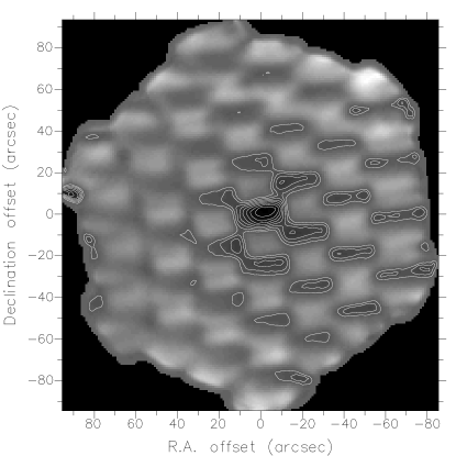
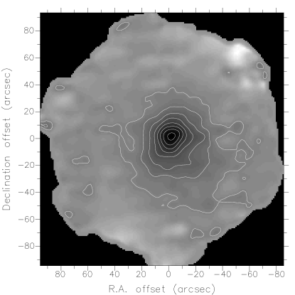
(a) (b) (c)

Figure 6: (a) Data processed without sky removal. (b) Image after sky contribution is removed from each jiggle position. The contour levels are as used in (a). (c) Plot showing data for the central pixel after sky removal and before sky removal along with the sky signal measured for the long and short wave arrays (lower two traces). Note that the data from the short-wave array has been reduced by a factor of 4 to bring it onto the same scale as the long-wave data.

3.2 Removing the effect of sky variability from SCUBA scan maps

The observing technique for scan mapping is to raster the SCUBA arrays over the map area, using the secondary chopper to measure the difference signal between points a short distance apart. Chopping removes the DC offset due to sky emission and diminishes the effect of sky variability on the signal. Unfortunately, it also results in a map that has the source profile convolved with the chop.

To restore the source profile we must deconvolve the chop from the measured map. The problems associated with this step can best be appreciated by considering the Fourier transform (FT) of the chop function, which is a sine wave with zeroes at the origin and at harmonics of the inverse chop throw. Deconvolving the chop function is equivalent to dividing the FT of the measured map by the FT of the chop and then transforming back to image space. Clearly, problems arise at spatial frequencies where the sine wave of the chop FT has a low value or is zero. Noise at these frequencies is blown up and significantly reduces the signal-to-noise of the restored map[7].

A few years ago Emerson[8] proposed a method by which this problem could be reduced and conducted tests on model data to demonstrate the improvement. His method requires the taking of 4 maps instead of 1; 2 maps chopping vertically with 2 different throws, and 2 chopping horizontally. The chop amplitudes are chosen so that, except at the origin, the zeroes in the FT of one do not coincide with the zeroes in the FT of the other up to the spatial frequency limit of the telescope beam. The 4 maps obtained are then Fourier transformed and coadded, each weighted in frequency space according to the sensitivity of its chop direction and throw. The coadd is transformed back to give the finished image.

This method has been used for SCUBA with very encouraging results. The final images are greatly improved cosmetically, are much less affected by spikes in the raw data and, most importantly, display a significant increase in signal-to-noise. An example of the improvement can be seen by comparing 2 maps of a large area around the nucleus of M82, the first taken with the old method (Fig. 7a), the second with the new (Fig. 7b), both with the same total integration time. In this case the signal-to-noise of the new map is 2 times better than the old.

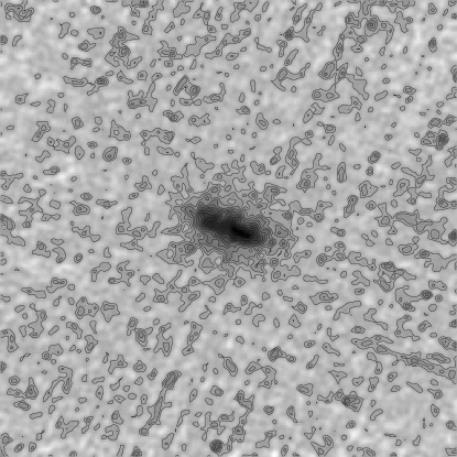
(a) (b)

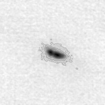
Figure 7: (a) This is a 256 arcsec by 256 arcsec map of M82 taken using the classic scan mapping technique[7] but with the addition of data from a second scanning angle. (b) This is a map of the same region with the same integration time, but taken and reduced according to the method described by Emerson[8]. Identical contour levels have been used.

There is, however, one problem evident in the new M82 map. Strong emission from the source is known to be restricted to a small area around the nucleus; the rest of the map should be empty. Instead we see small amplitude, large scale fluctuations around the zero level; to make this clearer the map is shown again in Fig. 10a with a colour table biased towards low intensity.

This residual noise is occurring at very low spatial frequencies, where all 4 chopped maps of the new method have low sensitivity. Even the new method of map restoration must inflate the signal at these frequencies to recover the source profile, along with any noise present. Unfortunately, it is at just such low frequencies that sky variability is likely to contribute most noise.

A small section of the raw data from one of the M82 observations is shown in Fig. 8a. In this we can clearly see small areas of high or low emission where bolometers have passed over the source. However, also visible are faint light and dark bands measured across all the bolometers simultaneously and with time-scales of order 1–20 seconds, characteristics both of variable sky emission.

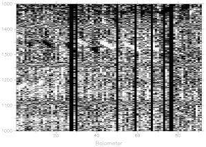
(a) (b)

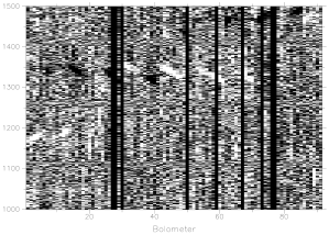
Figure 8: (a) A portion of the raw data from one of the observations of M82. Bolometer number increases along the x-axis and measurement number (time) up the y-axis. The measurements were made at approximately 8 Hz. (b) The same data after sky removal. Note that the faint banding visible across the bolometers in (a) (e.g. pixels 1050–1150 and pixels 1450–1500) has disappeared.

The main problem with removing sky variations from scan map data is that it is difficult to disentangle signals due to the sky from those due to passage over the source. In general, we would have to exploit the fact that source signals are correlated in position whereas sky variations correlate in time. However, our M82 dataset is a map covering a large area with a compact source at the centre so, in this case, we can cheat. It is possible to effectively remove the source from the raw data by simply ignoring all data points with a signal further from zero than a given threshold.

After source removal, a ‘variable sky’ dataset was calculated from the raw data by smoothing the time series signal from each bolometer with a box function 6 samples wide, then at each measurement time averaging the signal across all bolometers in the array with good noise behaviour. The variable sky was then subtracted from the original raw data resulting in a corrected dataset of which the same small section as before is plotted in Fig. 8b. It is evident that our crude efforts have been successful; the banding has disappeared in the corrected data and no new features have been added due to improper removal of source emission.

As an example of the strength of the sky variations compared to the raw signal from a single bolometer, the data for one bolometer over a short time-span are shown in Fig. 9. As can be seen, the sky variations are well below the noise level for the bolometer. Smoothing in time and averaging over the array are definitely required to measure the effect.

Figure 9: The raw time-series data for a single bolometer with, superimposed, the derived signal due to sky variation.

The method described above was used to remove the sky variations from all the M82 datasets and these were then reduced as before to yield the result shown in figure Fig. 10b. Here we can see that sky removal has indeed had the desired effect; the low frequency ripple on the background has all but disappeared.

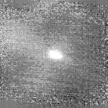
(a) (b)

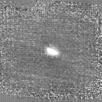
Figure 10: (a) Low intensity fluctuations in the map of M82 reduced without ‘sky removal’. (b) Map of M82 after ‘sky removal’, displayed on the same intensity scale as (a). The contour levels are the same for each image. These images cover a region of 500 arcsec by 500 arcsec.

And that completes the description of our work so far. Clearly, the method of sky removal outlined above is unsatisfactory for any but compact sources but it does demonstrate that further effort is very worthwhile. The next stage will be to develop a scheme by which extended sources of arbitrary shape can be removed from the raw data. One obvious method to try will be to calculate back from a reduced map the signal that should have been received at each measured position in the raw data, then subtract it from the actual raw data. Hopefully, this will be sufficiently accurate to leave the variable sky signal behind.

4 Conclusions

In this work we have shown that noise due to sky variability is evident in SCUBA data and that it is correlated across the array as well as at different wavelengths. This raises the prospect of using sky signal measured on one array to remove the sky signal measured on another. Currently the biggest issue facing us is that of sky removal for scan mapping; our preliminary investigation has shown that we can detect and remove this sky variability, albeit from compact sources.

References

- [1] W. D. Duncan, E. I. .Robson, P. A. R. Ade, and S. E. Church, “Measurements of submillimetre emission noise from Mauna Kea,” in Multi-feed Systems for Radio Telescopes, D. T. Emerson and J. M. Payne, eds., ASP Conference Series 75, pp. 295–308, 1995.
- [2] W. S. Holland, W. K. Gear, J. F. Lightfoot, T. Jenness, E. I. Robson, C. R. Cunningham, and K. Laidlaw, “SCUBA: A submillimetre camera operating on the James Clerk Maxwell Telescope,” in Advanced Technology MMW, Radio and Terahertz Telescopes, Proc. SPIE this volume, 1998.
- [3] C. R. Cunningham, W. K. Gear, W. D. Duncan, P. R. Hastings, and W. S. Holland, “SCUBA: The Submillimeter Common-User Bolometer Array for the James Clerk Maxwell Telescope,” in Instrumentation in Astronomy VIII, D. L. Crawford and E. R. Craine, eds., Proc. SPIE 2198, pp. 638–649, 1994.
- [4] W. K. Gear and C. R. Cunningham, “SCUBA: A camera for the James Clerk Maxwell Telescope,” in Multi-feed Systems for Radio Telescopes, D. T. Emerson and J. M. Payne, eds., ASP Conference Series 75, pp. 215–221, 1995.
- [5] J. F. Lightfoot, W. D. Duncan, W. K. Gear, B. D. Kelly, and I. A. Smith, “Observing strategies for SCUBA,” in Multi-feed Systems for Radio Telescopes, D. T. Emerson and J. M. Payne, eds., ASP Conference Series 75, pp. 327–334, 1995.
- [6] S. E. Church, A. N. Lasenby, and R. E. Hills, “An upper limit on the finescale anisotropy of the cosmic background radiation at 800-microns,” Mon. Not. R. Astron. Soc. 261, pp. 705–717, 1993.
- [7] D. T. Emerson, U. Klein, and C. G. T. Haslam, “A multiple beam technique for overcoming atmospheric limitations to single-dish observations of extended radio sources,” Astron. Astrophys. 76, pp. 92–105, 1979.
- [8] D. T. Emerson, “Approaches to multi-beam data analysis,” in Multi-feed Systems for Radio Telescopes, D. T. Emerson and J. M. Payne, eds., ASP Conference Series 75, pp. 309–317, 1995.