Constraining Large Scale Structure Theories
with the Cosmic Background Radiation

Abstract

The case is strong that cosmic microwave background (CMB) and large scale structure (LSS) observations can be combined to determine the theory of structure formation and the cosmological parameters that define it. We review: the relevant 10+ parameters associated with the inflation model of fluctuation generation and the matter content of the Universe; the relation between LSS and primary and secondary CMB anisotropy probes as a function of wavenumber; how COBE constraints on energy injection rule out explosions as a dominant source of LSS; and how current anisotropy band-powers in multipole-space, at levels $\sim(10^{-5})^{2}$, strongly support the gravitational instability theory and suggest the universe could not have reionized too early. We use Bayesian analysis methods to determine what current CMB and CMB+LSS data imply for inflation-based Gaussian fluctuations in tilted $\Lambda$CDM, $\Lambda$hCDM and $o$CDM model sequences with cosmological age 11-15 Gyr, consisting of mixtures of baryons, cold “c” (and possibly hot “h”) dark matter, vacuum energy “$\Lambda$”, and curvature energy “o” in open cosmologies. For example, we find the slope of the initial spectrum is within about 5% of the (preferred) scale invariant form when just the CMB data is used, and for $\Lambda$CDM when LSS data is combined with CMB; with both, a nonzero value of $\Omega_{\Lambda}$ is strongly preferred ($\approx 2/3$ for a 13 Gyr sequence, similar to the value from SNIa). The $o$CDM sequence prefers $\Omega_{tot}<1$, but is overall much less likely than the flat $\Omega_{\Lambda}\neq 0$ sequence with CMB+LSS. We also review the rosy forecasts of angular power spectra and parameter estimates from future balloon and satellite experiments when foreground and systematic effects are ignored to show where cosmic parameter determination can go with just CMB information alone.

1 The Relation Between CMB and LSS Observables

In this section, we first present an overview of the relation between the scales that CMB anisotropies probe, those that large scale structure observations of galaxy clustering probe, and the scales that are responsible for collapsed object formation in hierarchical models of structure formation, in particular those determining the abundances of clusters and galaxies. We review the basic parameters of amplitude and tilt characterizing the fluctuations in the simplest versions of inflation, but consider progressively more baroque inflation models needing progressively more functional freedom in describing post-inflation fluctuation spectra. We then describe the high precision that has been achieved in calculations of primary CMB anisotropies (those determinable with linear perturbation theory), and the less precisely calculable secondary anisotropies arising from nonlinear processes in the medium.

a CMB as a Probe of Early Universe Physics

The source of fluctuations to input into the cosmic structure formation problem is likely to be found in early universe physics. We want to measure the CMB (and large scale structure) response to these initial fluctuations. The goal is to peer into the physical mechanism by which the fluctuations were generated. The contenders for generation mechanism are (1) “zero point” quantum noise in scalar and tensor fields that must be there in the early universe if quantum mechanics is applicable and (2) topological defects which may arise in the inevitable phase transitions expected in the early universe.

From CMB and LSS observations we hope to learn: the statistics of the fluctuations, whether Gaussian or non-Gaussian; the mode, whether adiabatic or isocurvature scalar perturbations, and whether there is a significant component in gravitational wave tensor perturbations; the power spectra for these modes, ${\cal P}_{\Phi}(k),{\cal P}_{is}(k),{\cal P}_{GW}(k)$ as a function of comoving wavenumber $k=2\mathchar 28953\relax\bar{a}/\mathchar 28949\relax$, with the cosmological scale factor $\bar{a}(t)$ removed from the physical wavelength $\mathchar 28949\relax(t)$ and set to unity now. The length unit is ${\,{\rm h}^{-1}~{}\rm Mpc}$, where ${\rm h}$ is the Hubble parameter in units of $100{\rm~{}km~{}s^{-1}}{\rm~{}Mpc}^{-1}$, i.e., really a velocity unit. Until a few years ago ${\rm h}$ was considered to be uncertain by a factor of two or so, but is now thought to be between 0.6 and 0.7.

Sample initial and evolved power spectra for the gravitational potential ${\cal P}_{\Phi}(k)$ ($\equiv d\mathchar 28955\relax_{\Phi}^{2}/d\ln k$, the rms power per $d\ln k$ band) are shown in Fig. 1. The (linear) density power spectra, ${\cal P}_{\mathchar 28954\relax}(k)\propto k^{4}{\cal P}_{\Phi}(k)$, are also shown in Fig. 1. (We use ${\cal P}(k)=k^{3}P(k)/(2\mathchar 28953\relax^{2})$ for power spectra, the variance in the fluctuation variable per $\ln k$, rather than the oft-plotted mean-squared fluctuation for mode $k$, $P(k)$, so ${\cal P}_{\mathchar 28954\relax}\equiv\Delta^{2}(k)$ in the notation of Peacock (1997).) As the Universe evolves the initial shape of ${\cal P}_{\Phi}$ (nearly flat or scale invariant) is modified by characteristic scales imprinted on it that reflect the values of cosmological parameters such as the energy densities of baryons, cold and hot dark matter, in the vacuum (cosmological constant), and in curvature. Many observables can be expressed as weighted integrals over $k$ of the power spectra and thus can probe both density parameters and initial fluctuation parameters.

b Cosmic Structure and the Nonlinear Wavenumber

In hierarchical structure formation models such as those considered here, as the universe evolves ${\cal P}_{\mathchar 28954\relax}^{1/2}(k)$ grows with time until it crosses unity at small scales, and the first star forming tiny dwarf galaxies appear (“1st *”), typically at a redshift of about 20. The nonlinear wavenumber $k_{NL}(t)$, defined by $\int_{0}^{k_{NL}}{\cal P}_{\mathchar 28954\relax}(k)d\ln k$=1, decreases as the universe expands, leaving in its wake dwarf galaxies (dG), normal galaxies (gal), groups (gps) and clusters (cls), forming from waves concentrated in the $k$-space bands that their labels cover in Fig. 1. Equivalent mass scales are given above them.

Scales just below $k_{NL}$ are weakly nonlinear and define the characteristic patterns of filaments connecting clusters, and membranes connecting filaments. Voids are rare density minima which have opened up by gravitational dynamics and merged, opposite to the equally abundant rare density maxima, the clusters, in which the space collapses by factors of 5-10 and more.

At $k>k_{NL}(t)$, nonlinearities and complications associated with dissipative gas processes can obscure the direct connection to the early universe physics. Most easily interpretable are observables probing the linear regime now, $k<k_{NL}(t_{0})$. CMB anisotropies arising from the linear regime are termed primary. As Fig. 1 shows, these probe three decades in wavenumber, with the high $k$ cutoff defined by the physics at $z\sim 1000$ when CMB photons decoupled, not $k_{NL}$ at that time. Within the LSS band, two important scales for the CMB arise: the sound crossing distance at photon decoupling, $\sim 100{\,{\rm h}^{-1}~{}\rm Mpc}$, and the width of the region over which this decoupling occurs, which is about a factor of 10 smaller, and below which the primary CMB anisotropies are damped. LSS observations of galaxy clustering at low redshift probe a smaller range, but which overlaps the CMB range. We have hope that $z\sim 3$ LSS observations, when $k_{NL}(t)$ was larger, can extend the range, but gas dynamics can modify the relation between observable and power spectrum in complex ways. Although probes based on catalogues of high redshift galaxies and quasars, and on quasar absorption lines from the intergalactic medium, represent a very exciting observational frontier, it will be difficult for theoretical conclusions about the early universe and the underlying fluctuations to be divorced from these “gastrophysical” complications. Secondary anisotropies of the CMB (§ h), those associated with nonlinear phenomena, also probe smaller scales and the “gastrophysical” realm.

c Probing Wavenumber Bands with the CMB and LSS

Although the scales we can probe most effectively are smaller than the size of our Hubble patch ($\sim 3000{\,{\rm h}^{-1}~{}\rm Mpc}$), because ultralong waves contribute gentle gradients to CMB observables, we can in fact place useful constraints on the ultralarge scale structure (ULSS) realm “beyond our horizon”. Indeed current constraints on the size of the universe arise partly from this region and partly from the very large scale structure (VLSS) region. (For compact spatial manifolds, the wavenumbers have an initially discrete spectrum, and are missing ultralong waves, limited by the size of the manifold.)

The COBE data and CMB experiments with somewhat higher resolution probe the VLSS region very well. Density fluctuations are highly linear in that regime, which is what makes it so simple to analyze. One of the most interesting realms is the LSS one, in which CMB observations probe exactly the scales that LSS redshift surveys probe. The density fluctuations are linear to weakly nonlinear in this realm, so we can still interpret the LSS observations reasonably well — with one important caveat: Galaxies form and shine through complex nonlinear dissipative processes, so how they are distributed may be rather different than how the total mass is distributed. The evidence so far is consistent with this “bias” being only a linear amplifier of the mass fluctuations on large scales, albeit a different one for different galaxy types. Detailed comparison of the very large CMB and LSS redshift survey results we will get over the next five years should help enormously in determining the statistical nature of the bias.

Because the ${\cal P}_{\Phi}$ of the COBE-normalized sCDM model shown shoots high relative to the cluster data point, the sCDM model is strongly ruled out. More rigorous discussion of what is compatible with COBE, smaller angle CMB experiments such as SK95, the cluster data point and the shape of the ${\cal P}_{\Phi}$ spectrum as estimated from galaxy clustering data is given in § d. The filter functions plotted for SK95, Planck, etc. show the bands they are sensitive to: multiplying by a $k$-space $\Delta T/T$ power spectrum gives the variance per $\ln k$ (e.g., Bond 1996).

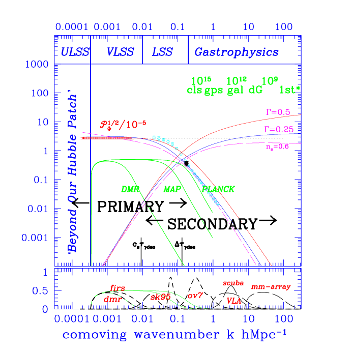
Figure 1: The bands in comoving wavenumber $k$ probed by CMB primary and secondary anisotropy experiments, in particular by the satellites COBE, MAP and Planck, and by large scale structure (LSS) observations are contrasted. The width of the CMB photon decoupling region and the sound crossing radius ($\Delta\mathchar 28956\relax_{\mathchar 28941\relax dec},c_{s}\mathchar 28956\relax_{\mathchar 28941\relax dec}$) define the effective acoustic peak range for primary anistropies (those involving linear fluctuations). Secondary anisotropies arise only once matter has gone nonlinear. Sample (linear) gravitational potential power spectra (actually ${\cal P}_{\Phi}^{1/2}(k)$) are also plotted, and the $y$-axis values refer to ${\cal P}_{\Phi}^{1/2}/10^{-5}$ (which is dimensionless). The horizontal dotted line is the post-inflation scale invariant power spectrum, which is bent down as the universe evolves by an amount dependent upon the matter content. The hatched region at low $k$ gives the 4 year DMR error bar on the $\Phi$ amplitude in the COBE regime. The solid data point in the cluster-band denotes the $\Phi$ constraint from the abundance of clusters (for $\Omega_{tot}$=1,$\Omega_{\Lambda}$=0). The open circles are estimates of the linear $\Phi$ power from current galaxy clustering data by Peacock (1997). A bias is “allowed” to (uniformly) raise the shapes to match the observations. The corresponding linear density power spectra, ${\cal P}_{\mathchar 28954\relax}^{1/2}(k)$, are also shown rising to high $k$. Models shown in Fig. 1 are the “standard” $n_{s}=1$ CDM model (labelled $\Gamma=0.5$ with $\Omega_{nr}=1$, ${\rm h}=0.5$), a tilted ($n_{s}=0.6$, $\Gamma=0.5$) CDM model and a model with the shape modified ($\Gamma=0.25$) by changing the matter content of the Universe, e.g., $\Omega_{nr}=0.36$, ${\rm h=0.7}$. The bands at high $k$ associated with object formation (cls, gal, etc. ) and the filters showing the bands various CMB experiments probe are discussed in the text.

d The Cosmic Parameters of Structure Formation Theories

Even simple Gaussian inflation-generated fluctuations for structure formation have a large number of early universe parameters we would wish to determine (§ e): power spectrum amplitudes at some normalization wavenumber $k_{n}$ for the modes present, $\{{\cal P}_{\Phi}(k_{n}),{\cal P}_{is}(k_{n}),{\cal P}_{GW}(k_{n})\}$; shape functions for the “tilts” $\{\mathchar 28951\relax_{s}(k),\mathchar 28951\relax_{is}(k),\mathchar 28951\relax_{t}(k)\}$, usually chosen to be constant or with a logarithmic correction, e.g., $\mathchar 28951\relax_{s}(k_{n}),d\mathchar 28951\relax_{s}(k_{n})/d\ln k$. (The scalar tilt for adiabatic fluctuations, $\mathchar 28951\relax_{s}(k)\equiv d\ln{\cal P}_{\Phi}/d\ln k$, is related to the usual index, $n_{s}$, by $\mathchar 28951\relax_{s}=n_{s}-1$.) The transport problem (§ g) is dependent upon physical processes, and hence on physical parameters. A partial list includes the Hubble parameter ${\rm h}$, various mean energy densities $\{\Omega_{tot},\Omega_{B},\Omega_{\Lambda},\Omega_{cdm},\Omega_{hdm}\}{\rm h}^{2}$, and parameters characterizing the ionization history of the Universe, e.g., the Compton optical depth $\mathchar 28956\relax_{C}$ from a reheating redshift $z_{reh}$ to the present. Instead of $\Omega_{tot}$, we prefer to use the curvature energy parameter, $\Omega_{k}\equiv 1-\Omega_{tot}$, thus zero for the flat case. In this space, the Hubble parameter, ${\rm h}=(\sum_{j}(\Omega_{j}{\rm h}^{2}))^{1/2}$, and the age of the Universe, $t_{0}$, are functions of the $\Omega_{j}{\rm h}^{2}$. The density in nonrelativistic (clustering) particles is $\Omega_{nr}=\Omega_{B}+\Omega_{cdm}+\Omega_{hdm}$. The density in relativistic particles, $\Omega_{er}$, includes photons, relativistic neutrinos and decaying particle products, if any. $\Omega_{er}$, the abundance of primordial helium, etc. should also be considered as parameters to be determined. The count is thus at least 17, and many more if we do not restrict the shape of ${\cal P}_{\Phi}(k)$ through theoretical considerations of what is “likely” in inflation models. Estimates of errors on a smaller 9 parameter inflation set for the MAP and Planck satellites are given in § e.

The arena in which CMB theory battles observation is the anisotropy power spectrum in multipole space, as in Figs. 2,3, which show how primary ${\cal C}_{\ell}$’s vary with some of these cosmic parameters. Here ${\cal C}_{\ell}\equiv\ell(\ell+1){\langle|(\Delta T/T)_{\ell m}|^{2}\rangle}/(2\mathchar 28953\relax)$. The ${\cal C}_{\ell}$’s are normalized to the 4-year dmr(53+90+31)(A+B) data (Bennett et al. 1996a, Bond 1995, Bond & Jaffe 1997). The arena for LSS theory battling observations is the ${\cal P}_{\Phi}$ of Fig. 1. (Usually it is ${\cal P}_{\mathchar 28954\relax}/k^{3}\sim k{\cal P}_{\Phi}$ which is plotted.)

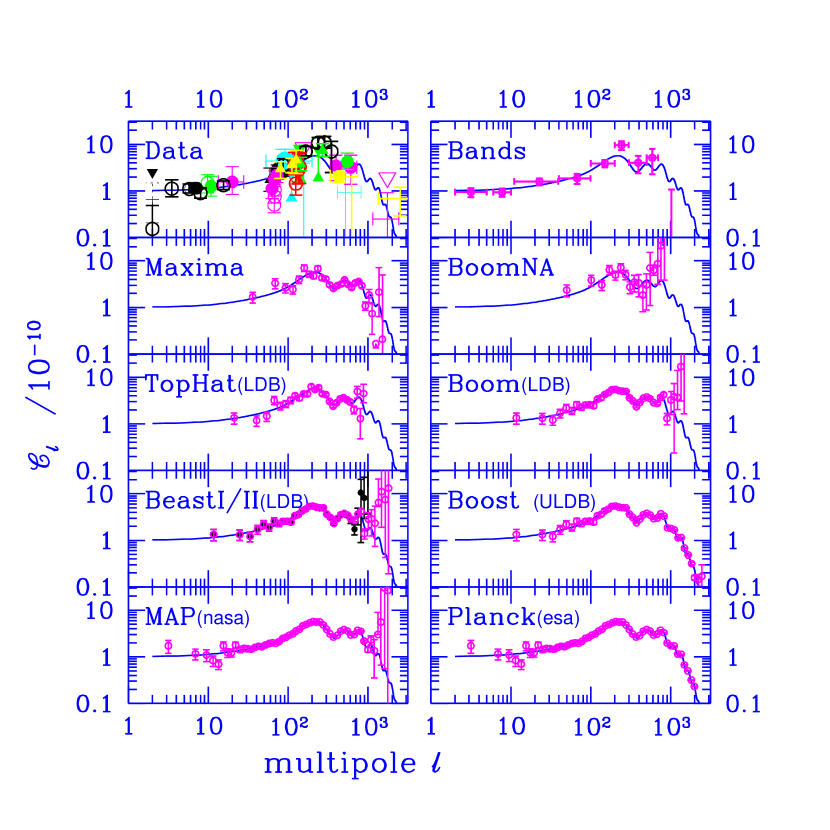
Figure 2: The ${\cal C}_{\ell}$ anisotropy bandpower data for experiments up to summer 1998 are shown in the upper left panel. The data are optimally combined into 9 bandpower estimates (with one-sigma errors) shown in the upper right panel. To guide the eye an untilted COBE-normalized sCDM model is repeated in all panels. The rest of the panels show forecasts of how accurate ${\cal C}_{\ell}$ will be determined for this model from balloon and satellite experiments, with parameters given in Table 2.

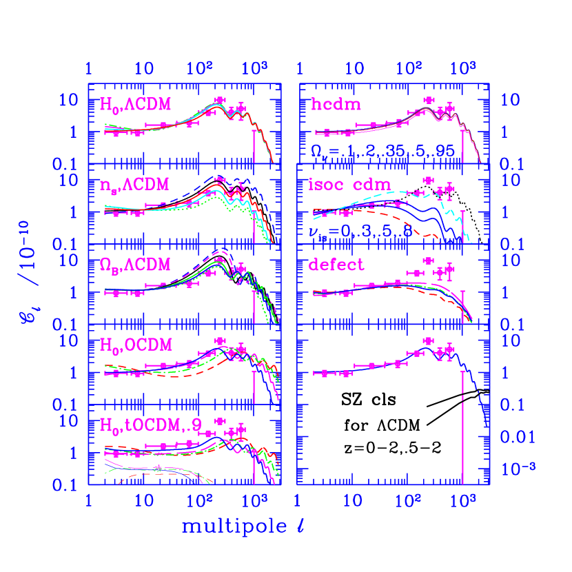
Figure 3: The 9 bandpower estimates from current anisotropy data are compared with various 13 Gyr model sequences: (1) $H_{0}$ from 50 to 90, $\Omega_{\Lambda}$, 0 to 0.87, for an untilted $\Lambda$CDM sequence; (2) $n_{s}$ from 0.85 to 1.25 for the $H_{0}=70$ $\Lambda$CDM model ($\Omega_{\Lambda}=.66$); (3) $\Omega_{B}{\rm h}^{2}$ from 0.003 to 0.05 for the $H_{0}=70$ $\Lambda$CDM model; (4) $H_{0}$ from 50 to 65, $\Omega_{k}$ from 0 to 0.84 for the untilted oCDM sequence; (5) the same for a $n_{s}=0.9$ oCDM sequence, clearly at odds with the data; (6) $H_{0}$=50 sequence with neutrino fractions varying from 0.1 to 0.95; (7) shows an isocurvature CDM sequence with positive isocurvature tilts ranging from 0 to 0.8; (8) shows that sample defect ${\cal C}_{\ell}$’s from Pen, Seljak and Turok (1997) do not fare well compared with the current data; ${\cal C}_{\ell}$’s from (Allen et al. 1997) are similar. The bottom right panel is extended to low values to show the magnitude of secondary fluctuations from the thermal SZ effect for the $\Lambda$CDM model. The kinematic SZ ${\cal C}_{\ell}$ is significantly lower. Dusty emission from early galaxies may lead to high signals, but the power is concentrated at higher $\ell$, with possibly a weak tail because galaxies are correlated extending into the $\ell\mathrel{\hbox to0.0pt{\lower 3.0pt\hbox{$\mathchar 536\relax$}\hss}\raise 2.0pt\hbox{$\mathchar 316\relax$}}2000$ regime.

For a given model, the early universe ${\cal P}_{\Phi}$ is uniquely related to late-time power spectrum measures of relevance for the CMB, such as the quadrupole ${\cal C}_{2}^{1/2}$ or averages over $\ell$-bands B, ${\langle{\cal C}_{\ell}\rangle}_{B}^{1/2}$, and to LSS measures, such as the rms density fluctuation level on the $8{\,{\rm h}^{-1}~{}\rm Mpc}$ (cluster) scale, $\mathchar 28955\relax_{8}$, so any of these can be used in place of the primordial power amplitudes in the parameter set. In inflation, the ratio of gravitational wave power to scalar adiabatic power is ${\cal P}_{GW}/{\cal P}_{\Phi}\approx-(100/9)\mathchar 28951\relax_{t}/(1-\mathchar 28951\relax_{t}/2)$, with small corrections depending upon $\mathchar 28951\relax_{s}-\mathchar 28951\relax_{t}$ (Bond 1994, 1996). If such a relationship is assumed, the parameter count is lowered by one.

e Fluctuation Freedom in Inflation

Many variants of the basic inflation theme have been proposed, sometimes with radically different consequences for ${\cal P}_{\Phi}(k)\sim k^{1-n_{s}(k)}$, and thus for the CMB sky, which is used in fact to highly constrain the more baroque models. A rank-ordering of inflation possibilities: (1) adiabatic curvature fluctuations with nearly uniform scalar tilt over the observable range, slightly more power to large scales ($0.8\mathrel{\hbox to0.0pt{\lower 3.0pt\hbox{$\mathchar 536\relax$}\hss}\raise 2.0pt\hbox{$\mathchar 316\relax$}}n_{s}\mathrel{\hbox to0.0pt{\lower 3.0pt\hbox{$\mathchar 536\relax$}\hss}\raise 2.0pt\hbox{$\mathchar 316\relax$}}1$) than “scale invariance” ($n_{s}=1$) gives, a predictable nonzero gravity wave contribution with tilt similar to the scalar one, and tiny mean curvature ($\Omega_{tot}\approx 1$); (2) same as (1), but with a tiny gravity wave contribution; (3) same as (1) but with a subdominant isocurvature component of nearly scale invariant tilt (the case in which isocurvature dominates is ruled out); (4) radically broken scale invariance with weak to moderate features (ramps, mountains, valleys) in the fluctuation spectrum (strong ones are largely ruled out); (5) radical breaking with non-Gaussian features as well; (6) “open” inflation, with quantum tunneling producing a negatively-curved (hyperbolic) space which inflates, but not so much as to flatten the mean curvature ($d_{c}\sim(Ha)^{-1}$, not $\gg(Ha)^{-1}$, where $d_{c}\equiv H_{0}^{-1}|\Omega_{k}|^{-1/2}$); (7) quantum creation of compact hyperbolic space from “nothing” with volume $d_{T}^{3}$ which inflates, with $d_{T}\sim(Ha)^{-1}$, not $\gg(Ha)^{-1}$, and $d_{T}$ of order $d_{c}$; (8) flat ($d_{c}=\infty$) inflating models which are small tori of scale $d_{T}$ with $d_{T}$ a few $(Ha)^{-1}$ in size. It is quite debatable which of the cases beyond (2) are more or less plausible, with some claims that (4) is supersymmetry-inspired, others that (6) is not as improbable as it sounds. Of course, how likely a priori the cases (7) and (8) of most concern to us here is completely unknown, but it is the theorists’ job to push out the boundaries of the inflation idea and use the data to select what is allowed.

f LSS Constraints on the Power Spectrum

We have always combined CMB and LSS data in our quest for viable models. Fig. 1 shows how the two are connected. DMR normalization precisely determines $\mathchar 28955\relax_{8}$ for each model considered; comparing with the $\mathchar 28955\relax_{8}\sim 0.6\Omega_{nr}^{-0.56}$ target value derived from cluster abundance observations severely constrains the cosmological parameters defining the models. In Fig. 1, this means the COBE-normalized ${\cal P}_{\Phi}(k)$ must thread the “eye of the needle” in the cluster-band.

Similar constrictions arise from galaxy-galaxy and cluster-cluster clustering observations: the shape of the linear ${\cal P}_{\Phi}$ must match the shape reconstructed from the data. The reconstruction shown is from Peacock (1997). The clustering observations are roughly compatible with an allowed range $0.15\mathrel{\hbox to0.0pt{\lower 3.0pt\hbox{$\mathchar 536\relax$}\hss}\raise 2.0pt\hbox{$\mathchar 316\relax$}}\Gamma+\mathchar 28951\relax_{s}/2\mathrel{\hbox to0.0pt{\lower 3.0pt\hbox{$\mathchar 536\relax$}\hss}\raise 2.0pt\hbox{$\mathchar 316\relax$}}0.3$, where $\Gamma\approx\Omega_{nr}\,{\rm h}\,[\Omega_{er}/(1.68\Omega_{\mathchar 28941\relax})]^{-1/2}\,e^{-(\Omega_{B}(1+\Omega_{nr}^{-1}(2{\rm h})^{1/2})-0.06)}$ characterizes the density transfer function shape. The sCDM model has $\Gamma\approx 0.5$. To get $\Gamma+\mathchar 28951\relax_{s}/2$ in the observed range one can: lower ${\rm h}$; lower $\Omega_{nr}$ ($\Lambda$CDM, oCDM); raise $\Omega_{er}$, the density parameter in relativistic particles ($1.68\Omega_{\mathchar 28941\relax}$ with 3 species of massless neutrinos and the photons), e.g., as in $\mathchar 28956\relax$CDM, with a decaying $\mathchar 28951\relax$ of lifetime $\mathchar 28956\relax_{d}$ and $\Gamma\approx 1.08\Omega_{nr}{\rm h}(1+0.96(m_{\mathchar 28951\relax}\mathchar 28956\relax_{d}/{\rm keV~{}yr})^{2/3})^{-1/2}$; raise $\Omega_{B}$; tilt $\mathchar 28951\relax_{s}<0$ (tCDM), for standard CDM parameters, e.g., $0.3\mathrel{\hbox to0.0pt{\lower 3.0pt\hbox{$\mathchar 536\relax$}\hss}\raise 2.0pt\hbox{$\mathchar 316\relax$}}n_{s}\mathrel{\hbox to0.0pt{\lower 3.0pt\hbox{$\mathchar 536\relax$}\hss}\raise 2.0pt\hbox{$\mathchar 316\relax$}}0.7$ would be required. Adding a hot dark matter component gives a power spectrum characterized by more than just $\Gamma$. In the post-COBE era, all of these models that lower $\Gamma+\mathchar 28951\relax_{s}/2$ have been under intense investigation to see which, if any, survive as the data improve.

g Cosmological Radiative Transport

Cosmological radiative transfer is on a firm theoretical footing. Together with a gravity theory (invariably Einstein’s general relativity, but the CMB will eventually be used as a test of the gravity theory) and the transport theory for the other fields and particles present (baryons, hot, warm and cold dark matter, coherent fields, i.e., “dynamical” cosmological “constants”, etc.), we propagate initial fluctuations from the early universe through photon decoupling into the (very) weakly nonlinear phase, and predict primary anisotropies, those calculated using either linear perturbation theory (e.g., for inflation-generated fluctuations), or, in the case of defects, linear response theory. The sources driving their development are all proportional to the gravitational potential $\Phi$: the “naive” Sachs-Wolfe effect, $\Phi/3$; photon bunching and rarefaction (acoustic oscillations), ${1\over 4}{\mathchar 28942\relax\mathchar 28954\relax_{\mathchar 28941\relax}\over\mathchar 28954\relax_{\mathchar 28941\relax}}$, responsible for the adiabatic ${1\over 3}{\mathchar 28942\relax\mathchar 28954\relax_{B}\over\mathchar 28954\relax_{B}}$ effect and the isocurvature effect; linear-order Thompson scattering (Doppler), $\mathchar 28955\relax_{T}\bar{n}_{e}{\bf v}_{e}\cdot{\hat{q}}$, with $\mathchar 28955\relax_{T}$ the Thomson cross section, ${\bf v}_{e}$ and $\bar{n}_{e}$ the electron velocity and density, and ${\hat{q}}$ the photon direction; the (line-of-sight) integrated Sachs-Wolfe effect, $\sim 2\int_{l.o.s.}\dot{\Phi}$; there are also subdominant anisotropic stress and polarization terms. For primary tensor anisotropies, the sources are the two polarization states of gravity waves, ${\textstyle{1\over 2}}\dot{h}_{+,\times}$; again there are subdominant polarization terms.

Spurred on by the promise of percent-level precision in cosmic parameters from CMB satellites (§ e), a considerable fraction of the CMB theoretical community with Boltzmann transport codes compared their approaches and validated the results to ensure percent-level accuracy up to $\ell\sim 3000$ (COMBA 1995). An important goal for COMBA was speed, since the parameter space we wish to constrain has many dimensions. Most groups have solved cosmological radiative transport by evolving a hierarchy of coupled moment equations, one for each $\ell$. Although the equations and techniques were in place prior to the COBE discovery for scalar modes, and shortly after for tensor modes, to get the high accuracy with speed has been somewhat of a challenge. There are alternatives to the moment hierarchy for the transport of photons and neutrinos. In particular the entire problem of photon transport reduces to integral equations in which the multipoles with $\ell>2$ are expressed as history-integrals of metric variables, photon-bunching, Doppler and polarization sources. The fastest COMBA-validated code, “CMBfast”, uses this method (Seljak & Zaldarriaga 1996), is publicly available and widely used (e.g., to generate some of the power spectra in Fig. 3).

h Secondary Anisotropies

Although hydrodynamic and radiative processes are expected to play important roles around collapsed objects and may bias the galaxy distribution relative to the mass (gastrophysics regime in Fig. 1), a global role in obscuring the early universe fluctuations by late time generation on large scales now seems unlikely. Not too long ago it seemed perfectly reasonable based on extrapolation from the physics of the interstellar medium to the pregalactic and intergalactic medium to suppose hydrodynamical amplification of seed cosmic structure could create the observed Universe. The strong limits on Compton cooling from the COBE FIRAS experiment (Fixsen et al. 1997), in energy ${\mathchar 28942\relax E_{Compton\ cool}/E_{cmb}}=4y<6.0\times 10^{-5}$ (95% CL), constrain the product $f_{exp}R_{exp}^{2}$ of filling factor $f_{exp}$ and bubble formation scale $R_{exp}$, to values too small for a purely hydrodynamic origin. If supernovae were responsible for the blasts, the accompanying presupernova light radiated would have been much in excess of the explosive energy (more than a hundred-fold), leading to much stronger restrictions (e.g., Bond 1996).

Nonetheless significant “secondary anisotropies” are expected. These include: linear weak lensing, dependent on the 2D tidal tensor, a projection of the 3D tidal tensor $\partial^{2}\Phi/\partial x^{i}\partial x^{j}$; the Rees-Sciama effect, $2\int_{l.o.s.}\dot{\Phi}_{NL}$, dependent upon the gravitational potential changes associated with nonlinear structure formation; nonlinear Thompson scattering, $\mathchar 28955\relax_{T}\mathchar 28942\relax{n}_{e}{\bf v}_{e}\cdot{\hat{q}}$, dependent upon the fluctuation in the electron density $\mathchar 28942\relax{n}_{e}$ as well as ${\bf v}_{e}$, and responsible for the quadratic-order (Vishniac) effect and the “kinematic” Sunyaev-Zeldovich (SZ) effect (moving cluster/galaxy effect); the thermal SZ effect, associated with Compton cooling, $\int_{l.o.s.}\mathchar 28960\relax_{K}(x)\mathchar 28942\relax(n_{e}T_{e})$, where $\mathchar 28960\relax_{K}(x)$ is a function of $x=E_{\mathchar 28941\relax}/T_{\mathchar 28941\relax}$ passing from $-2$ on the Rayleigh-Jeans end to $x$ on the Wein end, with a null at $x=2.83$ (i.e., $1863\mathchar 28950\relax{\rm m}$ or 161 GHz); pregalactic or galactic dust emission, $\sim\int_{l.o.s.}\mathchar 28960\relax_{dust}(x_{d})\mathchar 28954\relax_{d}$, dependent upon the distribution of the dust density $\mathchar 28954\relax_{d}$ and temperature $T_{d}$ through a function $\mathchar 28960\relax_{dust}$ of $x_{d}=E_{\mathchar 28941\relax}/T_{d}$.

Secondary anisotropies may be considered as a nuisance foreground to be subtracted to get at the primary ones, but they are also invaluable probes of shorter-distance aspects of structure formation theories, full of important cosmological information. The $k$-space range they probe is shown in Fig. 1. The effect of lensing is to smooth slightly the Doppler peaks and troughs of Fig. 3. ${\cal C}_{\ell}$’s from quadratic nonlinearities in the gas at high redshift are concentrated at high $\ell$, but for most viable models are expected to be a small contaminant. Thomson scattering from gas in moving clusters also has a small effect on ${\cal C}_{\ell}$ (although it should be measurable in individual clusters). Power spectra for the thermal SZ effect from clusters are larger (Bond & Myers 1996); the example in the bottom panel of Fig. 3 is for an untilted $H_{0}=70$ COBE-normalized $\Lambda$CDM model, with $\bar{y}\sim 2\times 10^{-6}\,(\Omega_{B}{\rm h}^{2}/0.025)$, still small c.f. the FIRAS constraint. (Here and in the following, when $H_{0}$ values are given, the units ${\rm~{}km~{}s^{-1}}{\rm~{}Mpc}^{-1}$ are implicit.) Although ${\cal C}^{(SZ)}_{\ell}$ may be small, because the power for such non-Gaussian sources is concentrated in hot or cold spots the signal is detectable, in fact has been for two dozen clusters now at the $>5$ sigma level, and indeed the SZ effect will soon be usable for cluster-finding. ${\cal C}_{\ell}$ for a typical dusty primeval galaxy model is concentrated at higher $\ell$ associated with galaxy sizes, although a small contribution associated with clustering extends into the lower $\ell$ range. These dusty anisotropies are now observable with instrumentation on submm telescopes (e.g., SCUBA on the James Clerk Maxwell Telescope on Mauna Kea, with the $k$-space filter shown in Fig. 1).

2 CMB Parameter Estimation, Current and Future

a Comparing and Combining CMB Experiments

We have progressed from the tens of pixels of early $\Delta T/T$ experiments through thousands for DMR (Bennett et al. 1996a) and SK95 (Netterfield et al. 1996), soon tens of thousands for long duration balloon experiments (LDBs) and eventually millions for the MAP (Bennett et al. 1996b) and Planck (Bersanelli et al. 1996) satellites. Finding nearly optimal strategies for data projection, compression and analysis which will allow us to disentangle the primary anisotropies from the Galactic and extragalactic foregrounds and from the secondary anisotropies induced by nonlinear effects will be the key to realizing the theoretically-possible precision on cosmic parameters and so to determine the winners and losers in theory space. Particularly powerful is to combine results from different CMB experiments and combine these with LSS and other observations. Application of the same techniques to demonstrate self-consistency and cross-consistency of experimental results is essential for validating conclusions drawn from the end-product of data analysis, e.g., the power spectra in bands as shown in Fig. 2 and the cosmic parameters they imply.

Current band-powers are shown in the upper panel of Fig. 2. The first lesson of Figs. 2,3 is that, in broad brush stroke, smaller angle CMB data (e.g., SP94, SK95, MSAM, MAX) are consistent with COBE-normalized ${\cal C}_{\ell}$’s for the untilted inflation-based models. It is possible that some of the results may still include residual contamination, but it is encouraging that completely different experiments with differing frequency coverage are highly correlated and give similar bandpowers, e.g. DMR and FIRS (e.g., Bond 1996), SK95 and MSAM (Netterfield et al. 1996, Knox et al. 1998). Lower panels compress the information into 9 optimal bandpower estimates derived from all of the current data (see Bond, Jaffe & Knox 1998b for techniques).

The few data points below $\ell\mathrel{\hbox to0.0pt{\lower 3.0pt\hbox{$\mathchar 536\relax$}\hss}\raise 2.0pt\hbox{$\mathchar 316\relax$}}20$ are mainly from COBE’s DMR experiment. Clearly the $\ell$-range spanned by DMR is not large enough to fix well the cosmological parameter variations shown in the right panels, but combining CMB anisotropy experiments probing different ranges in $\ell$-space improves parameter estimates enormously because of the much extended baseline: it is evident that $n_{s}$ can be reasonably well determined, low $\Omega$ open models violate the data, but $\Omega_{\Lambda}$ cannot be well determined by the CMB alone.

b DMR and Constraints on Ultra-large Scale Structure

DMR is fundamental to analyses of the VLSS region and ULSS region, and is the data set that is the most robust at the current time. The average noise in the 53+90+31 GHz map is about 20$\mathchar 28950\relax K$ per fwhm beam ($\sim 7^{\circ}$), and there are about 700 of these resolution elements outside of the Galactic disk cut (about 4000 2.6^∘ DMR pixels with 60$\mathchar 28950\relax K$ noise). The signal is about 37$\mathchar 28950\relax K$ per beam: i.e., there is a healthy signal-to-noise ratio. The signal-to-noise for widespread modes (e.g., multipoles with $\ell\mathrel{\hbox to0.0pt{\lower 3.0pt\hbox{$\mathchar 536\relax$}\hss}\raise 2.0pt\hbox{$\mathchar 316\relax$}}15$) is even better. Indeed, even with the much higher precision MAP and Planck experiments we do not expect to improve the results on the COBE angular scales greatly because the 4-year COBE data has sufficiently large signal-to-noise that one is almost in the cosmic variance error limit (due to realization to realization fluctuations of skies in the theories) which cannot be improved upon no matter how low the experimental noise.

Wiener-filtered maps shown in Fig. 4 give the statistically-averaged signal given the data and a best-fit signal model. These optimally-filtered maps are insensitive to modest variations in the assumed theory. The robustness of features in the maps as a function of frequency and the weak frequency dependence in the bandpowers are strong arguments that what is observed is on the sky with a primary anisotropy origin, made stronger by the compatible amplitudes and positive cross-correlations with the FIRS and Tenerife data sets.

Recall the “beyond our horizon” land in Fig. 1 is actually partly accessible because long waves contribute gentle gradients to our observables. The DMR data is well suited to probe this regime. Constraints on such “global parameters” as average curvature from COBE are not very good. Obviously it is much preferred to use the smaller angle data on the acoustic peak positions. The COBE data can be used to test whether radical broken scale invariance results in a huge excess or deficit of power in the COBE $k$-space band, e.g., just beyond $k^{-1}\sim H_{0}^{-1}$, but this has not been much explored. The remarkable non-Gaussian structure predicted by stochastic inflation theory would likely be too far beyond our horizon for its influence to be felt. The bubble boundary in hyperbolic inflation models may be closer and its influence shortly after quantum tunneling occurred could possibly have observable consequences for the CMB. Theorists have also constrained the scale of topology in simple models (Fig. 4). Bond, Pogosyan & Souradeep (1997, 1998) find the torus scale is $d_{T}/2>1.1(2H_{0}^{-1})=6600{\,{\rm h}^{-1}~{}\rm Mpc}$ from DMR for flat equal-sided 3-tori at the $95\%$ confidence limit, slightly better than other groups find since full map statistics were used. The constraint is not as strong if the repetition directions are asymmetric, $>0.7(2H_{0}^{-1})$ for 1-tori from DMR. It is also not as strong if more general topologies are considered, e.g., the large class of compact hyperbolic topologies (Bond, Pogosyan & Souradeep 1997, 1998, Cornish et al. 1996, 1998, Levin et al. 1997, 1998).

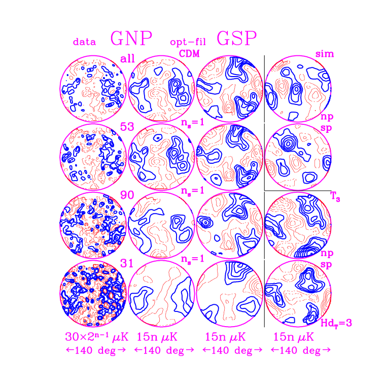
Figure 4: The first column shows unfiltered $140^{\circ}$ diameter dmr $A$+$B$ maps centered on the North Galactic Pole, the second shows them after Wiener-filtering (with monopole, dipole and quadrupole removed), the third the South Pole version, with the $nth$ contour as noted and negative contours heavier than positive ones. The Wiener maps use a model which fits the correlation function and amplitude of the DMR data (specifically, the $n_{s}$=1 sCDM model was used, but insensitive to even rather significant variations). The maps have been smoothed by a $1.7^{\circ}$ Gaussian filter. all is 53+90+31$A$+$B$. Although higher noise results in filtering on greater angular scales, the large scale features of all maps are the same. This is also borne out by detailed statistical comparisons map to map. The last column shows some theoretical realizations, after optimal filtering. The first two rows are the NGP and SGP for a $n_{s}$=1 CDM model. The lower two rows are for a 3-torus topology, with repetition length $d_{T}=9000{\,{\rm h}^{-1}~{}\rm Mpc}$, 1.5 times the horizon radius, in all three directions, a model strongly ruled out because of the high degree of positive correlation between the North and Southern hemispheres that the periodicity induces (Bond, Pogosyan & Souradeep 1998). Highly correlated patterns also exist for small compact hyperbolic models and lead to constraints on manifold size.

c Cosmic Parameters from All Current CMB Data

We have undertaken full Bayesian statistical analysis of the 4 year DMR (Bennet et al. 1996a), SK94-95 (Netterfield et al. 1996) and SP94 (Gundersen et al. 1995) data sets, taking into account all correlations among pixels in the data and theory (Bond & Jaffe 1997). Other experiments available up to March 1998 were included by using their bandpowers as independent points with the Gaussian errors shown in Fig. 2. We have shown this approximate method works reasonably well by comparing results derived for DMR+SP94+SK95 with the full analysis with those using just their bandpowers (Jaffe, Knox & Bond 1997). We have also shown that a significant improvement in accuracy is possible if instead of the average and 1 sigma limits on the experimental bandpowers ${\cal C}_{B}$ or on ${\cal C}_{B}^{1/2}$, one uses $\ln({\cal C}_{B}+x_{B})$, where $x_{B}$ is related to the noise of the experiment (Bond, Jaffe & Knox 1998b). This includes some of the major non-Gaussian deviations in the bandpower likelihood functions; results using this more accurate approach, and incorporating the very recent CAT98 and QMAP data, will be reported elsewhere (Bond, Jaffe & Knox 1998c, in preparation). Other groups have also calculated parameter constraints using the ${\cal C}_{B}^{1/2}$ bandpower approach (e.g., Lineweaver & Barbosa 1997, Hancock & Rocha 1997, Lineweaver 1998).

With current errors on the data, simultaneously exploring the entire parameter space of § d is not useful, so we restricted our attention to various subregions of $\{\Omega_{B}{\rm h}^{2},\Omega_{cdm}{\rm h}^{2},\Omega_{hdm}{\rm h}^{2},\Omega_{k}{\rm h}^{2},\Omega_{\Lambda}{\rm h}^{2},\mathchar 28951\relax_{s},\mathchar 28951\relax_{t},\mathchar 28955\relax_{8}\}$, such as $\{\mathchar 28955\relax_{8},n_{s},{\rm h}\,|\,{\rm fixed}\,t_{0},\Omega_{B}{\rm h}^{2}\}$, where $\Omega_{k}$=0 and $\Omega_{\Lambda}$ is a function of ${\rm h}t_{0}$ or $\Omega_{\Lambda}$=0 and $\Omega_{k}>0$ is a function of ${\rm h}t_{0}$. The age of the Universe, $t_{0}$, was chosen to be 11, 13 or 15 Gyrs. A recent estimate for globular cluster ages with the Hipparcos correction is $11.5\pm 1.3~{}{\rm Gyr}$ (Chaboyer et al. 1998), with perhaps another Gyr to be added associated with the delay in globular cluster formation, so 13 Gyr is a good example. We considered the ranges $0.5\mathrel{\hbox to0.0pt{\lower 3.0pt\hbox{$-$}\hss}\raise 2.0pt\hbox{$\mathchar 316\relax$}}n_{s}\mathrel{\hbox to0.0pt{\lower 3.0pt\hbox{$-$}\hss}\raise 2.0pt\hbox{$\mathchar 316\relax$}}1.5$, $0.43\mathrel{\hbox to0.0pt{\lower 3.0pt\hbox{$-$}\hss}\raise 2.0pt\hbox{$\mathchar 316\relax$}}{\rm h}\mathrel{\hbox to0.0pt{\lower 3.0pt\hbox{$-$}\hss}\raise 2.0pt\hbox{$\mathchar 316\relax$}}1$, and $0.003\mathrel{\hbox to0.0pt{\lower 3.0pt\hbox{$-$}\hss}\raise 2.0pt\hbox{$\mathchar 316\relax$}}\Omega_{B}{\rm h}^{2}\mathrel{\hbox to0.0pt{\lower 3.0pt\hbox{$-$}\hss}\raise 2.0pt\hbox{$\mathchar 316\relax$}}0.05$. The old “standard” nucleosynthesis estimate was $\Omega_{B}{\rm h}^{2}=0.0125$, but the preferred one is now $0.025$. We assumed reheating occurred sufficiently late to have a negligible effect on ${\cal C}_{\ell}$, although this is by no means clear. ${\cal C}_{\ell}$’s for sample restricted parameter sequences are shown in Fig. 3. We made use of signal-to-noise compression of the data (by factors of 3) in order to make the calculations of likelihood functions such as ${\cal L}(\mathchar 28955\relax_{8},n_{s},{\rm h}\,|\,{\rm fixed}\,t_{0},\Omega_{B}{\rm h}^{2})$ more tractable (without loss of information or accuracy).

The $n_{s}$ constraints are quite good. If $\mathchar 28955\relax_{8}$ is marginalized for the tilted $\Lambda$CDM sequence with $H_{0}$=50, with DMR only the primordial index is $n_{s}$ = $1.02^{+.23}_{-.25}$ with no gravity waves and $\mathchar 28951\relax_{t}$=0, and $1.02^{+.23}_{-.18}$ with gravity waves and $\mathchar 28951\relax_{t}$=$\mathchar 28951\relax_{s}$, rather encouraging for the nearly scale invariant models preferred by inflation theory. Because the gravitational potential changes at late time with $\Lambda\neq 0$, the integrated Sachs-Wolfe effect gives more power in ${\cal C}_{\ell}$ at small $\ell$, so the preferred $n_{s}$ steepens to compensate. When $\Lambda$ is marginalized in the 13 Gyr tilted $\Lambda$CDM sequence, $n_{s}=1.17\pm 0.31$ is obtained. For this sequence, when all of the current CMB data are used we get $1.02^{+.05}_{-.03}$ for $H_{0}=50$ (and $\Omega_{\Lambda}=0$, the tilted sCDM model sequence) and $1.00^{+.04}_{-.04}$ for $H_{0}=70$ (and $\Omega_{\Lambda}=0.66$). Marginalizing over $H_{0}$ (i.e., $\Lambda$) gives $1.01^{+.05}_{-.04}$ with gravity waves included, $0.98^{+.08}_{-.06}$ if they are not. The marginalized 13 Gyr tilted oCDM sequence gives $1.00^{+.05}_{-.05}$.

$H_{0}$ and $\Omega_{\Lambda}$ for fixed age are not that well determined by the CMB data alone, as can be seen from the dotted lines in Fig. 5. After marginalizing over all $n_{s}$, we get $H_{0}<75$ at $1\mathchar 28955\relax$, but effectively no constraint at 2$\mathchar 28955\relax$. The strong dependence of the position of the acoustic peaks on $\Omega_{k}$ means that the oCDM sequence is better restricted: $\Omega_{tot}\sim.7$ is preferred; for the 13 Gyr sequence this gives $H_{0}\approx 53$ and for the 11 Gyr sequence $H_{0}\approx 65$.

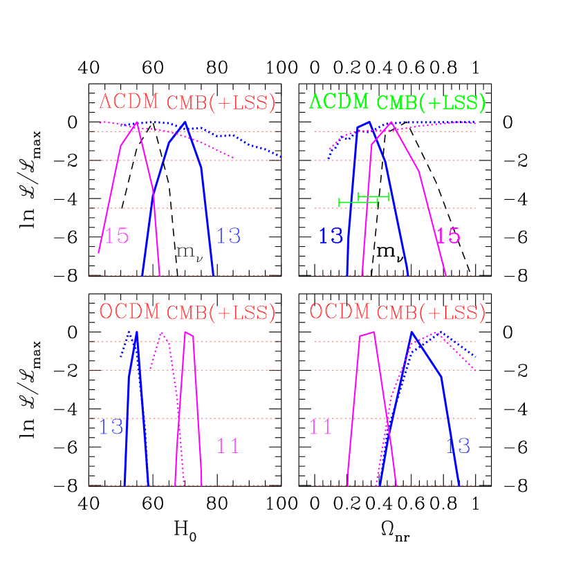
Figure 5: Likelihood curves for fixed-age $\Lambda$CDM and oCDM sequences, marginalized over $\mathchar 28955\relax_{8}$ and $n_{s}$. A Gaussian approximation to the likelihood places 1,2,3$\mathchar 28955\relax$ at the horizontal dashed lines. The 1$\mathchar 28955\relax$ ranges are explicitly given in the text. The dotted curves are for CMB only, solid for CMB+LSS. The right panels are equivalent to the left, but translated to $\Omega_{nr}$ ($1-\Omega_{\Lambda}$ for $\Lambda$CDM, $\Omega_{tot}$ for oCDM). The curves shown are for no GW, but there is little difference if GW are included. The sequence labelled $m_{\mathchar 28951\relax}$ is for the 13 Gyr $\Lambda$hCDM sequence with a fixed $\Omega_{m\mathchar 28951\relax}/\Omega_{nr}$ ratio of 0.2, and 2 degenerate neutrino species. Even this case favours slightly a nonzero $\Omega_{\Lambda}$. In the upper left panels, the 68% confidence limits for the values of $\Omega_{m}$ estimated using the luminosity-distance relation for Type I supernovae from Perlmutter et al. and Craig et al. are also shown. Note that the CMB data alone slightly favours a value of $\Omega_{tot}<1$. The absolute likelihood for the CMB+LSS data strongly favours the $\Lambda$CDM over the oCDM sequences. When just the fully analyzed DMR+SK95+SP94 data are used with LSS, the marginalized results for $\Lambda$CDM are remarkably similar, with the long baseline between DMR and SK95 fixing the freedom in $n_{s}$ (although values of $n_{s}$ about 1.1 are now preferred). When only DMR is used along with LSS, $n_{s}$ is not nailed down, and the resulting freedom implies $\Omega_{nr}=1$ models are not disfavoured. The horizontal error bars in the upper right panel show the $1\mathchar 28955\relax$ range of $\Omega_{nr}$ for $\Omega_{nr}+\Omega_{\Lambda}=1$ models inferred from the supernova Ia observations of Perlmutter et al. 1998 (upper) and Reiss et al. 1998 (lower).

Calculations of defect models (e.g. strings and textures) give ${\cal C}_{\ell}$’s that do not have the prominent peak that the data seem to indicate (Pen, Seljak & Turok 1997, Allen et al. 1997).

d Cosmic Parameters from Current LSS plus CMB Data

Combining LSS and CMB data gives more powerful discrimination among the theories, as Fig. 1 illustrates visually and Fig. 5 shows quantitatively. The approach we use here and in Bond & Jaffe (1997) to add LSS information to the CMB likelihood functions is to design prior probabilities for $\Gamma+\mathchar 28951\relax_{s}/2$ and $\mathchar 28955\relax_{8}\Omega_{nr}^{0.56}$, reflecting the current observations, but with flexible and generous non-Gaussian and asymmetric forms to ensure the priors can encompass possible systematic problems in the LSS data. For example, our choice for $\mathchar 28955\relax_{8}\Omega_{nr}^{0.56}$ was relatively flat over the 0.45 to 0.65 range. (Explicitly we used $0.55^{+.02+.15}_{-.02-.08}$, with the two error bars giving a Gaussian and a top hat error so that the net result is generously flat over the total $\pm 1\mathchar 28955\relax$ range. For $\Gamma+\mathchar 28951\relax_{s}/2$, we used $0.22^{+.07+.08}_{-.04-.07}$. Using the Peacock 1997 reconstructed linear power spectrum shown in Fig. 1 would give more stringent constraints for the shape e.g., Gawiser & Silk 1998.)

Using all of the current CMB data and the LSS priors, for the 13 Gyr $\Lambda$CDM sequence with gravity waves included, we get $n_{s}=1.00^{+.05}_{-.03}$ and $H_{0}=72\pm 3$ ($\Omega_{\Lambda}\approx 0.7$), respectively, when $H_{0}$ and $n_{s}$ are marginalized; with no gravity waves, $0.96^{+.07}_{-.05}$ and $H_{0}=70\pm 3$ are obtained; and for an $\Lambda$hCDM sequence, with a fixed ratio $\Omega_{hdm}/\Omega_{nr}=0.2$ for two degenerate massive neutrino species, $n_{s}\approx 0.97^{+.02}_{-.02}$ and $H_{0}\approx 57^{+5}_{-3}$ are obtained, revealing a slight preference for $\Omega_{\Lambda}\sim 0.3$. For the 15 Gyr $\Lambda$CDM sequence, the tilts remain nearly scale invariant and $\Omega_{\Lambda}$ near 0.6: $0.98^{+.04}_{-.03}$ and $H_{0}=57\pm 3$ ($\Omega_{\Lambda}\approx 0.6$) with gravity waves, $0.95^{+.05}_{-.05}$ and $54\pm 3$ ($\Omega_{\Lambda}\approx 0.5$) without.

For the 13 Gyr oCDM sequence, the likelihood peak for the CMB+LSS data is shifted relative to using the CMB data alone because the best fit CMB-only models have $\mathchar 28955\relax_{8}$ too low compared with the cluster abundance requirements. Although the $H_{0}\approx 54^{+1}_{-1}$ value ($\Omega_{tot}\approx 0.6$) is close to the CMB-only one, the maximum likelihood is significantly below the $\Lambda$CDM one. $H_{0}$ is larger for the 11 Gyr oCDM sequence, but $\Omega_{tot}$ is about the same, and the likelihood is still low.

Should these small error bars be taken seriously? It seems unlikely that $\mathchar 28955\relax_{8}$ from cluster abundances will change much; and, as we have seen, the DMR results are quite robust. Although largely driven by just the DMR plus LSS results, the smaller angle CMB results lock in the tilt, and as the CMB data improves some adjustment might occur, but not a drastic one unless we have made a major misinterpretation in the nature of the CMB signals observed at intermediate angles.

If we were to marginalize over $t_{0}$ as well, it is clear that $H_{0}$ would not be as well determined, but $n_{s}$ and either $\Omega_{k}$ or $\Omega_{\Lambda}$ would be. If the parameter space is made even larger, near degeneracies among some cosmic parameters become important for CMB data alone, and these are only partially lifted by the LSS data (e.g., Efstathiou & Bond 1998). In particular, this restricts the ultimate accuracy that can be achieved in the simultaneous determination of $\Omega_{k}$ and $\Omega_{\Lambda}$. This will become an issue when the quality of the CMB data improves, as described in the next subsection, but for now one must bear in mind the constrained space used when interpreting the current precision quoted on parameter estimation.

e Cosmic Parameters from the CMB Future

The expected error bars on the power spectrum from MAP and Planck (Bond, Jaffe & Knox 1998a, Bond, Efstathiou & Tegmark 1997, hereafter BET) shown in Fig. 2 illustrate that even quite small differences in the theoretical ${\cal C}_{\ell}$’s and thus the parameters can be distinguished. Quite an industry has developed forecasting how well future balloon experiments (Maxima, Boomerang, ACE, Beast, Top Hat), interferometers (VSA, CBI, VCA) and especially the satellites MAP and Planck could do in measuring the radiation power spectrum and cosmological parameters if foreground contamination is ignored (Knox 1995, Jungman et al. 1996, BET, Zaldarriaga, Spergel, & Seljak 1997, White, Carlstrom & Dragovan 1997). Forecasts like these were quite influential in making the case for MAP and Planck.

	Max	TH	BstI	II	Bm	Bm		MAP			Pl
$f_{sky}$	.01	.028	.067	.067	.02	.02	.67	.67	.67	.67	.67	.67
$\ell_{cut}$	20	12	6	6	12	12	2	2	2	2	2	2
$\mathchar 28951\relax$	all	all	40	90	90	150	90	60	40	100	150	220
$\mathchar 28946\relax_{fwhm}$	12	20	19	9	20	12	13	18	32	14.5	10	6.6
$\mathchar 28955\relax_{Npix}$	24	18.4	31	100	21	35	34	25	14	3.4	3.6	3.2

Table 1: The noise is per fwhm pixel, in $\mathchar 28950\relax$K. Max is Maxima, TH is TopHat, and Bst is Beast, which also has a 30 GHz channel ($26^{\prime}$, 53$\mathchar 28950\relax$K) included in the analysis. Bm is Boomerang, which also has 220 and 430 GHz channels not included in the analysis. The North America test flights covered .008 and .003 of the sky, and had fwhm of $35^{\prime}$ and $19^{\prime}$, respectively. Boost is a bolometer based version of Beast that is an example of an ultra-long duration balloon experiment, of order 100 days, with channels at 100 GHz ($9^{\prime}$, 17$\mathchar 28950\relax$K), 140 GHz($6^{\prime}$, 24$\mathchar 28950\relax$K), ($4^{\prime}$, 37$\mathchar 28950\relax$K), covering .07 of the sky, with $\ell_{cut}\approx 6$. The Planck numbers are for the HFI channels; a 350 GHz ($4^{\prime}$, 43$\mathchar 28950\relax$K) was also included in the analysis. See BET for the 3 channels of LFI used.

Param	Current	MaxTHBoom	MAP	Planck	Planck
	range	+BeastI+dmr		LFI	HFI
$f_{sky}$		0.07	0.67	0.67	0.67
$\mathchar 28942\relax n_{s}$	(0.5–1.5)	.07	.04	.01	.006
$\mathchar 28942\relax r_{ts}$	(0–1)	.55	.24	.13	.09
$\mathchar 28942\relax\Omega_{b}{\rm h}^{2}/\Omega_{b}{\rm h_{0}}^{2}$	(0.01–0.03)	.11	.05	.016	.006
$\mathchar 28942\relax\Omega_{m}{\rm h}^{2}/{\rm h_{0}}^{2}$	(.2-1)	.20	.10	.04	.02
$\mathchar 28942\relax\Omega_{\Lambda}{\rm h}^{2}/{\rm h_{0}}^{2}$	(0–0.8)	.46	.28	.14	.05
$\mathchar 28942\relax\Omega_{hdm}{\rm h}^{2}/{\rm h_{0}}^{2}$	(0–0.3)	.14	.05	.04	.02
$\mathchar 28956\relax_{C}$	(0.01–1)	.26	.19	.18	.16
$\mathchar 28942\relax{\rm h}/{\rm h}$	(40–80)	.15	.11	.06	.02
$\mathchar 28942\relax\Omega_{k}{\rm h}^{2}/{\rm h_{0}}^{2}$	(0.2–1.5)	.06	.04	.02	.007
Orthogonal Parameter Combinations within $\mathchar 28962\relax$
$\mathchar 28962\relax<0.01$	0/9	2/9	3/9	3/9	5/9
$\mathchar 28962\relax<0.1$	1/9	6/9	6/9	6/9	7/9

Table 2: Sample idealized MAP and Planck parameter error forecasts, for a 9 parameter inflation family of models, with standard CDM the “Target Model”. See BET for methods. $\Omega_{\Lambda}{\rm h}^{2}$ is determined with $\Omega_{k}{\rm h}^{2}$ fixed, and $\Omega_{k}{\rm h}^{2}$ is determined with $\Omega_{\Lambda}{\rm h}^{2}$ fixed, because of the angle-distance near-degeneracy (e.g., Efstathiou & Bond 1998); the other parameters are insensitive to fixing either, or neither. The ranges for $H_{0}$, $\Omega_{B}{\rm h}^{2}$ are absolute, but the errors are relative ones. The forecasted errors obviously represent a great leap forward from current errors and from what is conceivable with non-CMB probes. Amplitude parameters are highly correlated with $\mathchar 28956\relax_{C}$, but this can be partly broken when other information is included, e.g., on the abundance of clusters. The third column is an optimistic forecast of what one can do with balloons by combining MAXIMA, TopHat, Boomerang and BeastI with DMR (see Fig. 2). TopHat, Boomerang, and BeastI would be long duration balloon flights, lasting about a week over the Antarctic. The parameters used are given in Table 2. It is unclear that systematics will be sufficiently small for the LDB experiments to fulfill this promise.

Table 2 gives some examples of what can be obtained using only CMB data (BET). The experimental parameters chosen are given in Table 2. The durations chosen were appropriate for the types of experiments, e.g., about a week for long duration balloon experiments and about two years for satellite experiments. The temperature anisotropies were assumed to be Gaussian-distributed, and among the $>17$ parameters of § d, a restricted 9 parameter space was used: 5 densities, $\{\Omega_{B},\Omega_{nr},\Omega_{hdm},\Omega_{k},\Omega_{\Lambda}\}{\rm h}^{2}$, the Compton depth $\mathchar 28956\relax_{C}$, the scalar tilt, $n_{s}$, the total bandpower for the experiment ${\langle{\cal C}_{\ell}\rangle}_{B}$ in place of ${\cal P}_{\Phi}(k_{n})$, and the ratio of tensor to scalar quadrupole powers, ${r}_{ts}\equiv{{\cal C}^{(T)}_{2}/{\cal C}^{(S)}_{2}}$, in place of $\mathchar 28951\relax_{t}$. Just like ${\cal P}_{GW}/{\cal P}_{\Phi}$, ${r}_{ts}$ is a sensitive function of $\mathchar 28951\relax_{t}$, but also depends on $\mathchar 28951\relax_{s}-\mathchar 28951\relax_{t}$, $\Omega_{\Lambda}$, etc. (Bond 1996). In this space, recall that ${\rm h}^{2}=\sum_{j}(\Omega_{j}{\rm h}^{2})$ is a dependent quantity.

Except for the integrated Sachs-Wolfe effect at low $\ell$, the angular pattern of CMB anisotropies now is a direct map of the projected spatial pattern at redshift $\sim 100$, dependent upon the cosmological angle-distance relation, which is constant along a line relating $\Omega_{k}{\rm h}^{2}$ and $\Omega_{\Lambda}{\rm h}^{2}$ for fixed $\Omega_{nr}{\rm h}^{2}$. This defines a near-degeneracy between $\Omega_{k}$ and $\Omega_{\Lambda}$ broken only at low $\ell$ where the large cosmic variance precludes accurate determination of both parameters simultaneously (e.g. BET, Zaldarriaga, Spergel,& Seljak 1997, Efstathiou & Bond 1998, Eisenstein, Hu & Tegmark 1998). Other cosmological observables are needed to break this degeneracy. A good example is Type I supernovae. If they are assumed to be “standard candles”, then their degeneracy is along lines of equal luminosity-distance, which is sufficiently different from the equal angle-distance lines to allow good separate determination.

If the polarization power spectrum can be measured with reasonable accuracy, errors on some parameter such as $r_{ts}$ would improve (Zaldarriaga et al. 1997). However the polarization power spectrum is about a hundred times lower than the total anisotropy, and the gravity wave induced polarization is substantially tinier than this at the low $\ell$ needed for $r_{ts}$ improvement. We do not know if the foreground polarization will hopelessly swamp this signal.

Error forecasts do depend upon the correct underlying theory. In Table 2, untilted sCDM was chosen as the target model, but the values shown are indicative of what is obtained with other targets (BET). The third column gives errors forecasted for balloon experiments, the bolometer-based TopHat, Boomerang, and MAXIMA and the HEMT-based BEAST. (URLs to home pages are given in the references.) $\ell$-cuts were included to reflect the limited sky coverage these experiments will have. Adding DMR to extend the $\ell$-baseline diminishes the forecasted errors.

We adopt the current beam sizes and sensitivities for MAP and Planck used in BET, improvements over the original proposal values. Of the 5 HEMT channels for MAP, BET assumed the 3 highest frequency channels, at 40, 60 and 90 GHz, will be dominated by the primary cosmological signal (with 30 and 22 GHz channels partly contaminated by bremsstrahlung and synchrotron emission). MAP also assumes 2 years of observing. For Planck, BET used 14 months of observing, the 100, 65, 44 GHz channels for the HEMT-based LFI (but not the 30 GHz channel), and the 100, 150, 220 and 350 GHz channels for the bolometer-based HFI (but not the dust-monitoring 550 and 850 GHz channels). The highest resolution for MAP is $13^{\prime}$ fwhm, the highest for Planck is $4^{\prime}$.

These idealized error forecasts do not take into account the cost of separating the many components expected in the data, in particular Galactic and extragalactic foregrounds, but there is currently optimism that the Galactic foregrounds at least may not be a severe problem e.g., (Bersanelli et al. 1996), although low frequency emission near 100 GHz by small spinning dust grains (Leitch et al. 1997, Draine & Lazarian 1998) may emerge as a new significant source. There is more uncertainty about the extragalactic contributions in the submm and radio.

Although we may forecast wonderfully precise power spectra and cosmic parameters for the simplest inflation models in Table 2, once we consider the more baroque models with multifeatured spectra the precision drops(e.g., Souradeep et al. 1998). Given that all of our CMB and LSS observations actually access only a very small region of the inflation potential, imposing theoretical “prior” costs on highly exotic post-inflation shapes over the observable bands is reasonable. Nonetheless, if the phenomenology ultimately does teach us that non-baroque inflation and defect models fail, the CMB and LSS data will be essential for guiding us to a new theory of fluctuation generation.

We would like to thank George Efstathiou, Lloyd Knox, Dmitry Pogosyan, and Tarun Souradeep for enjoyable collaborations on a number of the projects highlighted in the text.

References

• Allen, B., Caldwell, R.R., Dodelson, S., Knox, L., Shellard, E.P.S. & Stebbins, A. 1997 preprint astro-ph/9704160.

• Beast home page, http://www.deepspace.ucsb.edu/research/Sphome.html

• Bennett, C. et al. 1996a Astrophys. J. Lett., 464, 1.

• Bennett C. et al. 1996b MAP home page, http://map.gsfc.nasa.gov

• Bersanelli, M. et al. 1996 COBRAS/SAMBA, The Phase A Study for an ESA M3 Mission, ESA Report D/SCI(96)3; Planck home page, http://astro.estec.esa.nl/SA-general/Projects/Cobras/cobras.html

• Bond, J.R. 1994 in Relativistic Cosmology, Proc. 8th Nishinomiya-Yukawa Memorial Symposium, ed. M. Sasaki, (Universal Academy Press, Tokyo), pp. 23-55.

• Bond, J.R. 1996 Theory and Observations of the Cosmic Background Radiation, in “Cosmology and Large Scale Structure”, Les Houches Session LX, August 1993, ed. R. Schaeffer, Elsevier Science Press, and references therein.

• Bond, J.R., Efstathiou, G. & Tegmark, M. 1997 Mon. Not. R. Astr. Soc. 291, L33 [BET].

• Bond, J.R. & Jaffe, A. 1997 in Microwave Background Anisotropies, Proceedings of the XXXI Rencontre de Moriond, ed. Bouchet, F R, Edition Frontières, Paris, pp. 197, astro-ph/9610091.

• Bond, J.R., Jaffe, A.H. & Knox, L. 1998a Phys. Rev. D 57, 2117.

• Bond, J.R., Jaffe, A.H. & Knox, L. 1998b Astrophys. J. submitted, astro-ph/9808264.

• Bond, J.R. & Myers, S. 1996 Astrophys. J. Supp. 103, 1-79.

• Bond, J.R., Pogosyan, D. & Souradeep, T. 1997 “Proc. 18th Texas Symposium on Relativistic Astrophysics”, 297-299, ed. A. Olinto, J. Frieman and D. Schramm (World Scientific, Singapore); 1998 Class. Quant. Grav. 15, in press; 1998 preprints, CITA-98-22, CITA-98-23.

• Boomerang home page, http://astro.caltech.edu/ mc/boom/boom.html

• Chaboyer, B., Demarque, P., Krauss, L.M. & Kernan, P.J. 1998 Astrophys. J. 494, 96.

• Bertschinger, E., Bode, P., Bond, J.R., Coulson, D., Crittenden, R., Dodelson, S., Efstathiou, G., Gorski, K., Hu, W., Knox, L., Lithwick, Y., Scott, D., Seljak, U., Stebbins, A., Steinhardt, P., Stompor, R., Souradeep, T., Sugiyama, N., Turok, N., Vittorio, N., White, M., Zaldarriaga, M. 1995 ITP workshop on Cosmic Radiation Backgrounds and the Formation of Galaxies, Santa Barbara.

• Cornish N.J., Spergel D.N. & Starkman G.D. 1996 preprint gr-qc/9602039; 1998 Class. Quant. Grav. 15, in press.

• Draine B.T. and Lazarian A. 1998 Astrophys. J. Lett. 494, 19.

• Efstathiou, G. & Bond, J.R. 1998, Mon. Not. R. Astr. Soc. submitted, astro-ph/9807103.

• Eisenstein, D.J., Hu, W. & Tegmark, M. 1998 preprint.

• Fixsen, D.J., Cheng E.S., Gales J.M., Mather J.C., Shafer R.A. & Wright E.L. 1997 Astrophys. J. 473, 576.

• Gawiser, E. & Silk, J. 1998 preprint.

• Gundersen J.O., Lim M., Staren J., Wuensche C.A., Figueiredo N., Gaier T.C., Koch T., Meinhold P.R., Seiffert M.D., Cook G., Segale A. & Lubin P.M. 1995 Astrophys. J. Lett. 443, L57-60.

• Jaffe, A.H., Knox, L. & Bond, J.R. 1997, “Proc. 18th Texas Symposium on Relativistic Astrophysics”, 273-275, ed. A. Olinto, J. Frieman and D. Schramm (World Scientific, Singapore), astro-ph/9702109.

• Jungman G., Kamionkowski M., Kosowsky A. & Spergel D.N. 1996 Phys. Rev. D54, 1332.

• Knox, L. 1995 Phys. Rev. D 52, 4307-4318.

• Knox, L., Bond, J.R., Jaffe, A.H., Segal, M. & Charbonneau, D. 1998 preprint.

• Leitch E.M., Readhead A.C.S., Pearson T.J., and Myers S.T. 1997 Astrophys. J. Lett. 486, 23.

• Levin J.J., Barrow J.D., Bunn E.F. and Silk J. 1997 Phys. Rev. Lett. 79 974; Levin J.J., Scannapieco E. and Silk J. 1998 Class. Quant. Grav. 15, in press.

• Lineweaver, C. and Barbosa, D. 1997 astro-ph/9706077.

• Lineweaver, C. 1998 preprint.

• Hancock, S. and Rocha, G. 1997, astro-ph/9612016, in Proceedings of the XVIth Moriond meeting, “Microwave Background Anisotropies,” ed. F.R. Bouchet et al.  (Gif-Sur-Yvette: Editions Frontières).

• MAXIMA home page, http://physics7.berkeley.edu/group/cmb/gen.html

• Netterfield, C.B., Devlin, M.J., Jarosik, N., Page, L. & Wollack, E.J. 1997 Astrophys. J.474, 47.

• Peacock J.A. 1997 Mon. Not. R. Astr. Soc. 284, 885.

• Pen, Ue-Li, Seljak, U. & Turok, N. 1997 preprint astro-ph/9704165.

• Perlmutter, S. et al. 1998 preprint.

• Reiss, A.G. et al. 1998 preprint astro-ph/9805201.

• Seljak U. & Zaldarriaga M. 1996 Astrophys. J.469, 437.

• Souradeep T., Bond J.R., Knox L., Efstathiou G., Turner M.S. 1998 astro-ph/9802262.

• Zaldarriaga M., Spergel, D. & Seljak U. 1997 preprint astro-ph/9702157.

• White M., Carlstrom J.E. and Dragovan M. 1997, astro-ph/9712195

• TopHat home page, http://cobi.gsfc.nasa.gov/msam-tophat.html